Fueling Low-Level AGN Activity Through the Stochastic Accretion of Cold Gas

Abstract

Using a simple description of feedback from black hole growth, we develop an analytic model for the fueling of Seyferts (low-luminosity AGN) and their relation to their host galaxies, Eddington ratio distributions, and cosmological evolution. We derive a solution for the time evolution of accretion rates in a feedback-driven blast wave, applicable to large-scale outflows from bright quasars in galaxy mergers, low-luminosity AGN, and black holes or neutron stars in supernova remnants. Under the assumption that cold gas stochastically accretes onto a central supermassive black hole at a rate set by the dynamics of that gas, our solution determines the evolution of Seyfert light curves. Using this model, we predict the Seyfert luminosity function, duty cycles and AGN “lifetimes,” and the distribution of host morphologies, Eddington ratios, and obscuration as a function of AGN luminosity and black hole mass, and find agreement with observations at $z=0$. We consider the breakdown of the contribution from this mechanism and from stellar wind and virialized hot gas accretion and merger-driven activity. We also make specific predictions for the weak evolution of the Seyfert luminosity function; i.e. luminosity function of quiescent, as opposed to merger-driven activity, as a function of redshift, and for changes in both the slope and scatter of the $M_{\rm BH}-\sigma$ relation at low-$M_{\rm BH}$. Our modeling provides a quantitative and physical distinction between local, low-luminosity quiescent AGN activity and violent, merger-driven bright quasars. In our picture, the quiescent mode of fueling dominates over a wide range of luminosities ($-14\gtrsim M_{B}\gtrsim-22$) at $z=0$, where most black hole growth occurs in objects with $M_{\rm BH}\lesssim 10^{7}\,M_{\sun}$, in S0 and Sa/b galaxies. However, quasar activity from gas-rich mergers evolves more rapidly with redshift, and by $z=1$, quiescent fueling is important only at luminosities an order of magnitude or more below the “break” in the luminosity function. Consequently, although non-merger driven fueling is important for black hole growth and the $M_{\rm BH}-\sigma$ relation at low $M_{\rm BH}$, it does not significantly contribute to the black hole mass density of the Universe or to cosmological backgrounds.

1. Introduction

While it is now generally accepted that quasars and active galactic nuclei (AGN) are powered by the accretion of gas onto supermassive black holes in the centers of galaxies (e.g. Salpeter 1964; Zel’dovich & Novikov 1964; Lynden-Bell 1969), the mechanism that fuels these objects is uncertain. In the local Universe, ultraluminous infrared galaxies (ULIRGs) have bolometric luminosities similar to bright quasars and are always in mergers (see e.g., Sanders et al., 1986, 1988; Soifer et al., 1987; Sanders & Mirabel, 1996), and multi-wavelength studies have shown that many contain growing, optically obscured black holes (Komossa et al., 2003; Gerssen et al., 2004; Max et al., 2005; Alexander et al., 2005a, b; Borys et al., 2005). Observations of low-redshift quasar hosts also reveal a connection between galaxy mergers and quasar activity (e.g., Heckman et al., 1984; Stockton & Ridgway, 1991; Hutchings & Neff, 1992; Bahcall et al., 1996, 1997; Canalizo & Stockton, 2001). These facts motivate a scenario where mergers of gas-rich galaxies provide the fuel to power nuclear starbursts which evolve into bright quasars.

Numerical simulations have identified a physical mechanism for transporting gas into the inner regions of galaxies in a merger by showing that tidally-induced gravitational torques remove angular momentum from the gas (e.g. Barnes & Hernquist 1991, 1996; Mihos & Hernquist 1996). Models including supermassive black holes (Di Matteo et al., 2005; Springel et al., 2005b) support the conjecture that ULIRGs evolve into quasars and suggest that feedback from black hole growth mediates this transition by expelling obscuring gas and dust. This “blowout” results in a short-lived, bright optical quasar (Hopkins et al., 2005a, b, 2006a) and eventually terminates the activity, leaving a remnant that quickly reddens (e.g. Springel et al. 2005a) and satisfies observed correlations between black hole mass and the mass (Magorrian et al., 1998; McLure & Dunlop, 2002; Marconi & Hunt, 2003) or velocity dispersion (i.e. the $M_{\rm BH}$-$\sigma$ relation: Ferrarese & Merritt 2000; Gebhardt et al. 2000) of spheroids.

Moreover, the time evolution in these simulations reproduces many quasar observables, including luminosity functions, host properties, and accretion rates (Hopkins et al., 2005c, d, 2006a, 2006c). The modeling also indicates that the bright quasar population and the bulk of the cosmic quasar luminosity density and buildup of the black hole mass density must be dominated by merger-driven growth (Hopkins et al., 2005e), to be consistent with the evolution of the X-ray background (Hopkins et al., 2006a), the red galaxy age, metallicity, mass, and luminosity functions (Hopkins et al., 2006b), and merger luminosity functions and star formation rate densities (Hopkins et al., 2006e).

However, many local, low-luminosity AGN reside in quiescent, non-interacting galaxies (e.g., Kauffmann et al., 2003a; Sánchez & González-Serrano, 2003; Sánchez et al., 2004; McLure & Dunlop, 2004; Hao et al., 2005). Some of these objects do in fact fit naturally into a merger-driven picture. At relatively high luminosities, ellipticals with young stellar populations and moderate Eddington ratios have observed properties consistent with decay in the quasar light curve from a previous bright quasar epoch in a spheroid-forming merger (Kauffmann et al., 2003a; Best et al., 2005; Hopkins et al., 2005e, 2006c). At the lowest luminosities characteristic of low-luminosity AGN and LINERs, populations of very low accretion rate “dead” ellipticals dominate, fueled via accretion of hot (virialized) spheroid gas and steady mass loss from stars (e.g., Ciotti & Ostriker, 1997, 2001; Pellegrini, 2005; Soria et al., 2005b), presumably in radiatively inefficient accretion states (e.g., Narayan & Yi, 1995). Although the detailed properties of these objects are subject to debate (see, e.g., Narayan, 2004), the fuel source is reasonably well-understood, and it is clear from comparison of black hole mass and quasar luminosity functions (e.g., Soltan, 1982; Salucci et al., 1999; Yu & Tremaine, 2002; Marconi et al., 2004; Shankar et al., 2004), background synthesis models (e.g., Comastri et al., 1995; Gilli et al., 1999; Elvis et al., 2002; Ueda et al., 2003; Cao, 2005), and observations of the accretion rate distribution (Vestergaard, 2004; Heckman et al., 2004; McLure & Dunlop, 2004; Hopkins et al., 2005e) that these modes do not dominate black hole growth or cosmological backgrounds.

Nevertheless, a number of relatively high accretion rate objects are observed at low redshift in undisturbed, late-type, star-forming galaxies (e.g., Kauffmann et al., 2003a) with small ($M_{\rm BH}\lesssim 10^{7}\,M_{\sun}$) black holes (Heckman et al., 2004). Indeed, the local AGN population largely comprises black holes in non-interacting, star-forming S0 and Sa/b hosts with no evidence of galaxy-scale perturbations or disturbances (Dong & De Robertis, 2005), spanning most of the observed $z=0$ AGN luminosity function (Hao et al., 2005). Although these AGN have been more thoroughly studied and are more well-understood than bright quasars at high redshift, there is no self-consistent model for their triggering, fueling, and evolution. Previous investigations of their fueling have mainly been restricted to estimating whether or not a given fuel source could provide an adequate mass supply (e.g., Lynden-Bell, 1969; Hills, 1975; Shields & Wheeler, 1978; Mathews, 1990), or have examined the evolution of light curves in limited subclasses of these objects (e.g., Ciotti & Ostriker, 2001). A critical uncertainty in previous efforts to model AGN is the light curve evolution once a given “trigger” occurs.

Independent of how fuel is delivered to the supermassive black holes in Seyferts and low-luminosity AGN, their subsequent evolution may resemble that in bright quasars if feedback from accretion regulates black hole growth. In the simulations of Di Matteo et al. (2005), the impact of this feedback resembles an explosion because the energy is deposited on scales small compared to the host galaxy and because the black hole grows nearly exponentially during the quasar phase with an e-folding time that is short compared to the characteristic dynamical time of the host potential. Indeed, Hopkins et al. (2005g) show that the outflow driven by this feedback can be described as a blast wave. In what follows, we investigate whether solutions of this type can also be used to characterize the evolution of low-luminosity AGN and Seyferts.

There is observation evidence for outflows and winds in both AGN and quasars (for a review, see Veilleux et al., 2005). The kinematics of gas in the narrow line regions of local, low-luminosity AGN (see, e.g. Rice et al., 2006, and references therein) display bi-conical or nearly isotropic (wide-angle) radial outflows at speeds $\sim 10^{2}-10^{3}\,{\rm km\,s^{-1}}$ (e.g., Crenshaw et al., 2000), with wind dynamical times $\sim 10^{4}-10^{6}\,$yr and entrained molecular gas masses $\sim 10^{5}-10^{7}\,M_{\sun}$ (e.g., Stark & Carlson, 1984; Walter et al., 2002). The “warm absorber” seen in soft X-rays is also indicative of a significant outflow generated local to the AGN (e.g., Laor et al., 1997, and references therein), accelerating radially to larger terminal velocities $\gtrsim{\rm a\ few\ }100\,{\rm km\,s^{-1}}$ (Ruiz et al., 2001; Kaspi et al., 2002). These absorbing outflows appear ubiquitous (and are likely even where not directly observed, given observed wind covering angles and clumping factors; see e.g. Rupke et al., 2005) and are associated with clumpy, high-ionization structures (e.g., Crenshaw et al., 1999). Outflow energetics and entrained masses appear to scale with AGN power (Baum & McCarthy, 2000), and intense winds with velocities $\sim 10^{4}\,{\rm km\,s^{-1}}$ are seen in bright, broad absorption line (BAL) quasars (e.g., Reeves et al., 2003). Observations of typical, narrow-line quasars also find BAL-like outflow velocities for some species accelerating at small radii from the central engine (Pounds et al., 2003a, b), and outflows with large covering angles in central regions of “normal” quasars may even be detected in gravitational lensing signatures (Green, 2006).

Although the relative contributions of star formation and AGN to the energetics is unclear (see e.g., Baum et al., 1993; Levenson et al., 2001), high-resolution data indicate that even Seyfert II ULIRGs in which large-scale winds may be driven by star formation have central, AGN-driven outflows (Cecil et al., 2001; Rupke et al., 2005), and observations at optical, X-ray, and radio wavelengths (Colbert et al., 1996a, b, 1998; Whittle & Wilson, 2004) identify a number of mechanisms by which AGN power can couple to outflows over $\sim$kpc scales. The decomposition of the narrow line region components also suggests wind ram pressure or radiation pressure from the central source as a driver (Kaiser et al., 2000), and in some cases the wind injection zone is observed to be small relative to the scale of nuclear star formation (Smith & Wilson, 2001). Furthermore, similar outflow structures are observed in the hot gas of some spheroidal systems which have no rapid associated star formation (e.g., Biller et al., 2004; Fabbiano et al., 2004).

The various observations fit naturally into a picture where outflows are caused by feedback from AGN accretion. This has motivated theoretical studies of the properties of AGN winds (e.g., Shlosman, Vitello, & Shaviv, 1985; Narayan & Yi, 1994; Konigl & Kartje, 1994; Stone & Norman, 1994; Murray et al., 1995; Elvis, 2000; Proga et al., 2000; Proga & Kallman, 2004). The models have invoked various driving mechanisms near the black hole, including hydromagnetic disk winds (e.g., Konigl & Kartje, 1994), MHD jet outflows (e.g., Blandford & Payne, 1982) powered by magnetic coronae formation over the disk (Miller & Stone, 2000), Comptonization in an X-ray halo (e.g., Begelman, 1985), and radiation pressure coupling to dust opacity (e.g., Dopita et al., 2002). Irrespective of their details, these processes universally yield a multi-temperature, clumpy, filled wind structure (Begelman & McKee, 1983; Konigl & Kartje, 1994) which provides a good representation of the various components and spectral properties of observed outflows (e.g., Krolik & Kriss, 2001; Dopita et al., 2002; Ogle et al., 2003). The winds evolve like a Sedov-Taylor type blast wave (Begelman et al., 1983), as suggested by observed velocity profiles (Shopbell & Bland-Hawthorn, 1998), and develop the typical shell structure and phases of evolution of these blast waves (Schiano, 1985), well known from the analysis of supernova remnants (e.g., Ostriker & McKee, 1988).

The theoretical works have examined the generation mechanisms of winds near a pre-existing accretion disk, and the observable impact of these winds on the interstellar medium (ISM) as they shock and entrain gas (e.g., Middelberg et al., 2004; Machacek et al., 2004; O’Sullivan et al., 2005). However, the AGN luminosity or accretion rate is generally an input parameter in these analyses, with an undetermined macroscopic fueling mechanism. Without a self-consistent calculation of the coupled evolution of the wind/blast wave and AGN accretion rate, such models, while critical for characterizing the detailed radiative properties of the ISM local to the AGN, cannot provide a physical motivation or understanding of the distribution of AGN luminosities, Eddington ratios, black hole masses, and fueling mechanisms, and their evolution with redshift.

If feedback from accretion couples to the gas surrounding black holes in Seyferts, the observations and theoretical models motivate the following picture for AGN activity in quiescent galaxies having a supply of cold gas. Observations of the dynamics and distribution of cold gas in the central regions of these AGN (e.g., Krolik & Begelman, 1988; Kaneko et al., 1989; Heckman et al., 1989; Israel et al., 1989; Meixner et al., 1990; Granato et al., 1997; Bock et al., 2000; Schinnerer et al., 2000; Galliano et al., 2003; Radomski et al., 2003; Weigelt et al., 2004; Jaffe et al., 2004; Prieto et al., 2004; Elitzur, 2005; Mason et al., 2005) suggest that rotationally supported gas extends to the inner regions of the galaxy. Whether part of the galactic disk or, potentially, a “clumpy” torus (e.g., Antonucci, 1993) or bar-like structure, molecular clouds or blobs of cold gas could be accreted stochastically by the black hole. Such gas will have some turbulent (random) motion and corresponding probability of colliding with the central black hole (see also e.g. Lauer et al., 2005).

The mass of gas required to sustain an AGN is only $\sim 10^{5}-10^{7}\,M_{\sun}$, far less than the $\sim 10^{8}-10^{9}\,M_{\sun}$ observed within the inner tens to hundreds of pc of many late-type galaxies (e.g., Kaneko et al., 1989; Heckman et al., 1989; Meixner et al., 1990; Granato et al., 1997; Galliano et al., 2003; Mason et al., 2005; Elitzur, 2005, and references therein), and only $\sim 1$ event per Hubble time may be expected (see § 4.2). Therefore, large-scale gravitational torques are not required, although mechanisms such as disk and bar instabilities (e.g., Norman & Silk, 1983; Norman & Scoville, 1988; Shlosman, Begelman, & Frank, 1989; Lin, Pringle, & Rees, 1988; Lubow, 1988), minor mergers (e.g., Roos, 1981; Gaskell, 1985; Hernquist, 1989; Mihos & Hernquist, 1994; Hernquist & Mihos, 1995; De Robertis et al., 1998; Tanaguchi, 1999), or magnetic instabilities (e.g., Krolik & Meiksin, 1990) may contribute to the “effective” turbulent motion. In a “collision,” the black hole will accrete at a high rate for a brief period of time until feedback impacts the cold gas, driving a blast wave and initiating a feedback-dominated “blowout” phase. This blowout determines the subsequent, time-averaged evolution of the Seyfert light curve, obscured fractions, and Eddington ratio distributions, and the system decays to lower luminosities until a potential subsequent excitation.

We use this picture to develop a model for the fueling of Seyfert galaxies, which allows us to predict their luminosity functions and evolution with redshift, among other quantities. In § 2, we derive a generalized Sedov-Taylor solution for feedback-driven outflows and both a Bondi-Hoyle type and generalized perturbative accretion solution within such a medium. This is applicable to any feedback regulated accretion system, including the quiescent systems studied here, “blowouts” in merger-driven quasars, and accreting black holes and neutron stars in supernova blast waves. In § 3 we apply this solution to the cases of merger-driven activity and stochastic accretion in quiescent systems. In § 4 we calculate the expected excitation rates, duty cycles, and luminosity function of Seyfert galaxies as triggered in quiescent galaxies. We further predict and compare with observations the distribution of host properties and morphological types as a function of luminosity, the distributions of accretion rates and Eddington ratios, and evolution (compared to e.g. evolution in merger-driven quasar activity) with redshift. In § 5 we predict the effects on the $M_{\rm BH}-\sigma$ relation from this mode of AGN fueling, in particular estimating corrections to the slope and scatter at low $M_{\rm BH}$. In § 6 we determine the implications of this picture for Seyfert obscuration and the potential buildup of the classical molecular torus. In § 7 we investigate effects on the host galaxy from this mode of fueling. In § 8 we estimate and compare with other quiescent modes of AGN fueling, such as accretion of hot spheroid gas and stellar winds from passive evolution. Finally, in § 9 we summarize and discuss predictions to test our model.

2. Accretion in Feedback-Driven Outflows

A black hole accreting at the Eddington rate will grow exponentially on a relatively short timescale (a few $\times 10^{7}\,$yr). If the black hole is small, feedback is suppressed exponentially, and surrounding gas can equilibrate with the low rate of energy or momentum input. However, if the black hole is already large, it will be sufficiently luminous that the energy injected cannot be radiated by the gas in a local dynamical time, effectively resulting in an instantaneous, point-like (relative to the scales of the galaxy) energy injection in the center of an (approximately spherical) bulge which dominates the local gravitational potential. Therefore, it is appropriate to describe this phase as a Sedov-Taylor type blast wave, which, in detail, a number of simulations have shown is a surprisingly good approximation to a full solution including radiative cooling, the pressure of the external medium, magnetic and gravitational fields, and further effects, at least on galaxy (Hopkins et al., 2006c) and larger (Furlanetto & Loeb, 2001) scales.

Here, we determine the behavior of such a blast wave when energy is input from black hole accretion into a medium with an initial density gradient. In particular, we derive an approximation to the internal density, velocity, and temperature structure of the blast wave as a function of time, which becomes exact as $r\rightarrow 0$. Using this, we can calculate the evolution of the Bondi-Hoyle accretion rate for a central black hole at $r=0$. However, because the Bondi rate is not calculated self-consistently in a medium with external density and velocity gradients, we use our solution for the internal blast wave structure to derive a solution for a perturbative inflow driven by the black hole gravitational potential at small radii.

Many authors have considered the evolution of blast waves and the detailed clumping and radiative properties of their interiors (e.g., Begelman et al., 1983; Begelman & McKee, 1983; Ostriker & McKee, 1988, and references therein). (For a discussion of the different Sedov-Taylor radial shells or phases see e.g. Schiano (1985).) However, these works have focused on understanding the radiative properties of such blast waves, and have not calculated an accretion rate solution within them or examined the interior properties as they affect the small radii relevant for accretion processes.

For simplicity, we assume a power-law scaling for the external (pre-shock) density,

$$\rho_{0}(r)\propto{R}^{-k_{\rho}}\,,$$ (1)

appropriate for a spheroid or black hole-dominated potential or molecular cloud. Note that this need hold only over some range in $r$ for each “stage” of the blast wave. We are, for now, interested in early times during the wave and (by definition of the blowout “triggering” condition) blast waves with energy greater than the binding energy of the material, so at least in this phase we can consider gravity to be a second-order effect which we calculate in detail below.

Under these circumstances, the system will evolve as a similarity solution, in which the shock radius $R_{s}$ expands as

$$R_{s}\propto t^{\eta}.$$ (2)

These similarity solutions are well-understood, and we refer to Ostriker & McKee (1988) for details. Once the system enters the blast wave-dominated phase, the central accretion rate will decline with time, in power-law fashion when the surrounding medium evolves according to a similarity solution. We derive this below; for now note that we expect

$$L\propto\dot{M}\propto t^{-\eta_{L}}$$ (3)

with $\eta_{L}\geq 0$. The total energy of the blast wave evolves as

$$E_{s}\propto R_{s}^{-k_{E}}\propto t^{\eta_{E}}$$ (4)

with $\eta_{E}=-\eta\,k_{E}$. Radiative losses from the blast wave front are small, at least on the scales of interest here (Furlanetto & Loeb, 2001). However, if feedback energy continues to couple to the surrounding medium as the accretion rate declines, there are two possible cases. First, if

$$\eta_{L}\geq 1,\ \eta_{E}\approx 0,$$ (5)

then the blast wave is dominated by the initial energy input, and the evolution is effectively energy conserving with $k_{E}=0$. Second, if

$$0\leq\eta_{L}<1,\ \eta_{E}={1-\eta_{L}},$$ (6)

the energy input increases with time and radius in a self-similar manner. In either case, we obtain a similarity solution for the shock radius of the form

$$\eta=\frac{2}{5-k_{\rho}+k_{E}}=\frac{2+\eta_{E}}{5-k_{\rho}}.$$ (7)

2.1. Internal Blast Wave Structure at Small Radii

We determine the internal structure of the blast wave using the two-power approximation (TPA) for the internal velocity and density structure. Unlike e.g. a one-power approximation, this ensures that gradients behave physically at small radii. In general, a quantity $x$ will have the scaling

$$x(r,\,t)=x_{1}(R_{s})\,\tilde{x}(\lambda)$$ (8)

internal to the blast wave, where

$$\lambda=r/R_{s}$$ (9)

and $x_{1}$ is the post-shock value of $x$ at the shock front. From Ostriker & McKee (1988), this gives

$$\tilde{\rho}=a_{\rho}\lambda^{\ell_{\rho 1}}+(1-a_{\rho})\,\lambda^{\ell_{\rho 2}}$$ (10)

where

$${\ell_{\rho 1}=\frac{3-\gamma\,k_{\rho}}{\gamma-1}=\frac{1}{2}(9-5k_{\rho})}$$

$${a_{\rho}=\frac{\gamma(k_{\rho,\,{\rm crit}}-k_{\rho})}{10-\gamma-(\gamma+2)k_{\rho}}=\frac{5(2-k_{\rho})}{25+11\,k_{\rho}}}$$

$${\ell_{\rho 2}={\rm MIN}(\frac{6-(g+1)(2\,k_{\rho}-k_{\rho,\,{\rm crit}})}{\gamma-1},\ell_{\rho 1},1)=17-8\,k_{\rho}}$$

$${k_{\rho,\,{\rm crit}}=\frac{7-\gamma}{\gamma+1}=2}$$ (11)

(the second equalities are for $\gamma=5/3$). These are determined by requiring the gradients to match exact solutions at the center and shock front and imposing mass conservation. The corresponding velocity approximation is

$$\tilde{v}=\frac{(\gamma+1)\lambda+(\gamma-1)\lambda^{\ell_{v2}}}{2\gamma}=\frac{4}{5}\lambda+\frac{1}{5}\lambda^{\ell_{v2}}$$ (12)

with

$$\ell_{v2}=1+\frac{\gamma}{\gamma-1}(k_{\rho,\,{\rm crit}}-k_{\rho})=6-\frac{5}{2}k_{\rho}.$$ (13)

The expressions reduce to an exact solution for $\gamma=5/3$, $k_{\rho}=k_{\rho,\,{\rm crit}}=2$. For other cases, they provide a good approximation for our purposes, accurate to $\sim 17\%$ even for $k_{\rho}=0$. The accuracy improves at small radii, and these solutions capture the correct power-law dependence as $r\rightarrow 0$ where, for example, Kahn’s approximation (Kahn, 1976) for the density and velocity structure, which is accurate to $\sim 4\%$ (Cox & Franco, 1981) reduces to the expressions above. These also provide a good description of observed blast wave velocity and temperature structure (e.g., Shopbell & Bland-Hawthorn, 1998; Crenshaw et al., 2000; Krolik & Kriss, 2001; Smith & Wilson, 2001; Kaspi et al., 2002; Veilleux et al., 2005; Rice et al., 2006).

Given the density and velocity field, it is straightforward to determine the interior pressure. For an adiabatic blast wave, the entropy per unit mass is conserved in comoving coordinates, giving

$$s\equiv P/\rho^{\gamma}=s_{1}\tilde{M}^{\ell_{s}}$$

$$M(r)=M\,\tilde{M}(\lambda)$$

$$\ell_{s}=\frac{\gamma k_{\rho}-3-k_{E}}{3-k_{\rho}}\,.$$ (14)

This yields

$$P\propto\lambda^{\frac{\gamma}{\gamma-1}\frac{5-k_{\rho}}{2+\eta_{E}}\eta_{E}}$$ (15)

for the pressure as $P\rightarrow 0$. For a blast wave with no energy injection, then, we recover the well-known condition that the pressure is constant at the origin.

In detail, we can use the equation of motion to solve for the pressure terms. Inserting the density and velocity fields into the equation of motion and solving yields a six-term power-law solution for the pressure

$$\frac{P}{\rho_{1}v_{1}^{2}} = a_{P0}+a_{P1}\,\lambda^{\ell_{\rho 1}+2}+a_{P2}\,\lambda^{\ell_{\rho 2}+2}$$ (16)

$$\mbox{}+a_{P3}\,\lambda^{\ell_{\rho 1}+\ell_{v}+1}+a_{P4}\,\lambda^{\ell_{\rho 2}+\ell_{v}+1}$$

$$\mbox{}+a_{P5}\,\lambda^{\ell_{\rho 1}+2\,\ell_{v}}+a_{P6}\,\lambda^{\ell_{\rho 2}+2\,\ell_{v}}$$

with

$$a_{P1}=\frac{a_{\rho}a_{v}(1-a_{v}\eta\nu_{1})}{(2+\ell_{\rho 1})\eta\nu_{1}}$$

$$a_{P2}=\frac{(a_{\rho}-1)a_{v}(1-a_{v}\eta\nu_{1})}{(2+\ell_{\rho 2})\eta\nu_{1}}$$

$$a_{P3}=\frac{a_{\rho}(a_{v}-1)(-1+\eta-\ell_{v}\eta+a_{v}(1+\ell_{v})\eta\nu_{1})}{(1+\ell_{\rho 1}+\ell_{v})\eta\nu_{1}}$$

$$a_{P4}=\frac{(1-a_{\rho})(a_{v}-1)(-1+\eta-\ell_{v}\eta+a_{v}(1+\ell_{v})\eta\nu_{1})}{(1+\ell_{\rho 2}+\ell_{v})\eta\nu_{1}}$$

$$a_{P5}=\frac{-a_{\rho}(1-a_{v})^{2}\ell_{v}}{\ell_{\rho 1}+2\ell_{v}}$$

$$a_{P6}=\frac{(a_{\rho}-1)(1-a_{v})^{2}\ell_{v}}{\ell_{\rho 2}+2\ell_{v}}\,,$$ (17)

where $a_{v}=(\gamma+1)/(2\gamma)$ is the coefficient of the $\lambda$ term in $\tilde{v}$ and $\nu_{1}\equiv v_{1}/v_{s}=2/(\gamma+1)$.

Because $P=P_{1}$ at $\lambda=1$, we obtain a solution for $a_{P0}$. In terms of $\tilde{P}$

$$\tilde{P}=\tilde{P}(0)+a_{\tilde{P}}\lambda^{\ell_{\rho 1}+2}+...$$ (18)

this yields an expression for $\tilde{P}(0)$ which is quite complicated, reducing for e.g. $k_{E}=0$, $\gamma=5/3$ to

$$\tilde{P}(0) = \frac{1}{175}{\Bigl{(}}82+\frac{210}{23-10\,k_{\rho}}+\frac{266}{19-8\,k_{\rho}}$$ (19)

$$+\frac{7}{11-5\,k_{\rho}}-\frac{560}{13-5\,k_{\rho}}-\frac{108}{16-7\,k_{\rho}}{\Bigr{)}}\,,$$

which interpolates from $\tilde{P}(0)\approx 0.32$ for $k_{\rho}=0$ to $\tilde{P}(0)=1/25$ for $k_{\rho}=2$. However, the full expression for $\tilde{P}(0)$ from the six-power expansion is reasonably well approximated (to $\sim 10\%$ for a variety of $\gamma,\ k_{\rho},\ k_{E}$) by the simpler form

$$\tilde{P}(0) = \frac{(\gamma+1)^{2}(k_{\rho,\,{\rm crit}}-k_{\rho}-k_{E})}{3\gamma^{2}+20\gamma+1-(\gamma+1)[(3\gamma+1)\,k_{\rho}-3(\gamma-1)\,k_{E}]}$$ (20)

$$= \frac{4\,(3-k_{\rho}-k_{E})}{24-9\,k_{\rho}+6\,k_{E}}\,,$$

which follows from the pressure-gradient approximation (see Ostriker & McKee, 1988), essentially a two-power approximation in the pressure.

The next-order term, $a_{\tilde{P}}\lambda^{\ell_{\rho 1}+2}$, which is proportional to the local $\rho v^{2}$, is given by

$$a_{\tilde{P}} = \frac{(\gamma^{2}-1)(k_{\rho,\,{\rm crit}}-k_{\rho})((5-k_{\rho})\gamma-(2+\eta_{E}))}{2\gamma(1+(2-k_{\rho})\gamma)\,(10-\gamma-(2+\gamma)\,k_{\rho})\,(2+\eta_{E})}$$ (21)

$$= \frac{8(2-k_{\rho})(19-5k_{\rho}-3\eta_{E})}{5(13-5k_{\rho})(25-11k_{\rho})(2+\eta_{E})}.$$

This goes to zero for $\gamma=5/3$, $k_{\rho}\rightarrow 2$, but this is because in this case $a_{\rho}\rightarrow 0$, $\ell_{\rho 1}=\ell_{\rho 2}=1$, and a proper solution yields

$$a_{\tilde{P}}=\frac{2-\eta_{E}}{2+\eta_{E}}\,.$$ (22)

It is straightforward to derive the remaining terms, but we are interested only in the behavior as $r\rightarrow 0$, so we do not need higher-order terms in $\lambda$.

2.2. Evolution of the Bondi Approximation

We can now determine the Bondi accretion rate as a function of radius, again for $r\rightarrow 0$, given by

$$\dot{M}=\frac{4\pi\alpha G^{2}\,M_{\rm BH}^{2}\,\rho}{(v^{2}+c_{s}^{2})^{3/2}},$$ (23)

where $\alpha$ is a constant of order unity dependent on the gas equation of state, $\rho$ and $c_{s}^{2}\equiv\gamma P/\rho$ are the local gas density and sound speed, respectively and $v$ is the bulk motion of the gas relative to the black hole. Near the origin, $\tilde{P}\rightarrow\tilde{P}(0)=\,$constant, thus

$$P(0)=\tilde{P}(0)P_{1}=\tilde{P}(0)\theta_{0}\rho_{0}(R_{s})v_{s}^{2}$$

$$\theta_{0}=\frac{2}{\gamma+1}$$

$$\rho\rightarrow a_{\rho}\lambda^{\ell_{\rho 1}}\rho_{1}=a_{\rho}\chi_{1}\lambda^{\ell_{\rho 1}}\rho_{0}(R_{s})$$

$$\chi_{1}=\frac{\gamma+1}{\gamma-1}$$

$$c_{s}^{2}=\frac{\gamma\tilde{P}(0)\theta_{0}}{a_{\rho}\chi_{1}}\,\lambda^{-\ell_{\rho 1}}\,v_{s}^{2}$$

$$\frac{\rho}{c_{s}^{3}}=\chi_{1}{\Bigl{(}}\frac{\gamma\tilde{P}(0)\theta_{0}}{a_{\rho}\chi_{1}}{\Bigr{)}}^{-3/2}\,{\Bigl{(}}\frac{r}{R_{s}}{\Bigr{)}}^{\frac{5}{2}\ell_{\rho 1}}\frac{\rho_{0}(R_{s})}{v_{s}(R_{s})^{3}}$$

$$\ \ \ \ \propto r^{\frac{5}{2}\ell_{\rho 1}}t^{3\,(1-\eta)-\eta(k_{\rho}+\frac{5}{2}\ell_{\rho 1})}.$$ (24)

So, at some point, an inward-moving Bondi-like flow can grow and give a residual accretion rate, and if the shock wave continues to blow mass out of the central regions, the scaling should be similar to the time scaling above. The effective “accretion radius” at which this will occur is, however, ambiguous. A natural choice is the black hole radius of influence,

$$R_{\rm BH}=\frac{G\,M_{\rm BH}}{\sigma^{2}}$$ (25)

where $\sigma$ is the bulge velocity dispersion. This follows from equating the black hole potential to the external potential, and determines where the black hole dominates the dynamics. We could instead consider the trans-sonic radius,

$$R_{\rm ts}=\frac{G\,M_{\rm BH}}{c_{s}(R_{\rm ts})^{2}}\,;$$ (26)

however, once $c_{s}(R_{\rm BH})<\sigma$, the trans-sonic radius will be larger than the black hole radius of influence, regardless of how $c_{s}$ scales with $R$, and the black hole will not affect the dynamics. For the inner regions (or intermediate regions for $k_{\rho}=2,\ \gamma=5/3$), we have $c_{s}\sim v\sim r/t$, so $R_{\rm ts}\gtrsim R_{\rm BH}$ at $t\sim R_{\rm BH}/\sigma\sim\mu\,t_{\rm dyn}$, where

$$\mu\equiv\frac{M_{\rm BH}}{M_{\ast}}\approx 0.001$$ (27)

is the ratio of the black hole to the (total) spheroid stellar mass (e.g., Marconi & Hunt, 2003) and

$$t_{\rm dyn}\equiv\frac{a}{\sigma}\approx 3.6\times 10^{7}\,{\rm yr}\ {\Bigl{(}}\frac{\sigma}{100\,{\rm km\,s^{-1}}}{\Bigr{)}}$$ (28)

is defined as the spheroid dynamical time (with $a$ being the bulge scale length). Thus the timescale for $R_{\rm ts}\gg R_{\rm BH}$ is $\sim 10^{4}$ yr, much less than the timescales of interest, and so it is inappropriate to consider accretion through $R_{\rm ts}$ as it is outside the region where the black hole will have a significant effect on the kinematics. Even if some of the post-shock gas avoids cooling adiabatically and slows/compresses to pressure equilibrium, this will necessarily give $c_{s}\sim\sigma$, so $R_{\rm ts}\sim R_{\rm BH}$ and again $R_{\rm BH}$ is the appropriate radius to consider.

Since we expect the accretion rate to decline rapidly with time, the black hole mass is approximately constant over this period (see § 5.4 for a detailed calculation), so for a fixed accretion radius $\sim R_{\rm BH}$ this then gives

$$\dot{M}\propto\frac{\rho}{c_{s}^{3}}\propto t^{3\,(1-\eta)-\eta(k_{\rho}+\frac{5}{2}\ell_{\rho 1})}\propto t^{-\eta_{L}}.$$ (29)

This equation for $\eta_{L}$ expands to

$$\eta_{L}=\frac{24-9\gamma-5\,k_{\rho}}{(\gamma-1)\,(5-k_{\rho})}=\frac{3(9-5k_{\rho})}{2(5-k_{\rho})}$$ (30)

for a rapidly declining accretion rate with $\eta_{E}=0$ (i.e. valid for $\eta_{L}>1$, $k_{\rho}<17/13$ for $\gamma=5/3$). For a less rapidly declining accretion rate with $\eta_{E}\neq 0$ (i.e. $0<\eta_{L}<1$) we obtain a self-consistent solution with

$$\eta_{L}=\frac{3\,(19-4\gamma-(4+\gamma)\,k_{\rho})}{(16-5\,k_{\rho})\gamma-1}=\frac{111-51\,k_{\rho}}{77-25\,k_{\rho}}\,,$$ (31)

which is valid for all $k_{\rho}$ where $\eta_{L}<1$ ($k_{\rho}>17/13$ for $\gamma=5/3$). Together, these form a continuous class of self-consistent solutions for all $0\leq k_{\rho}\leq 37/17$.

2.3. Perturbative Calculation of the Accretion Rate

Although the above derivation gives a reasonable solution for $\dot{M}$ and its scaling with time, in agreement with simulations (Hopkins et al., 2006c), it is not strictly appropriate to adopt the Bondi-Hoyle rate at some radius, as the full blast wave solution represents an outflow. However, in the Sedov-Taylor solution, a given mass shell interior to the blast wave decelerates with time, and eventually the gravitational potential will dominate the dynamics. Shells with smaller initial $r/R_{s}$ begin with smaller relative velocities and decelerate more quickly, and will successively “turn around” and fall back establishing a Bondi-Hoyle-like steady accretion flow. Therefore, we expect a mode of inflow in the inner regions which grows relative to the decaying blast wave solution, with the inflow smaller at early times when the blast wave is propagating rapidly (although the inflow may decay with time in an absolute sense). The gravitational term in the equation of motion is a perturbation, which will induce corresponding perturbations in the velocity and density. We can, therefore, describe this inflow as a perturbation about the exact blast wave solution. We consider the density and velocity perturbations $\delta_{\rho}\ll\rho$ and $\delta_{v}\ll v$, and demand that the first order perturbation to the mass inflow rate

$$\delta{\dot{M}}=\delta{\dot{M}}(t)=4\,\pi\,r^{2}\,(\delta_{\rho}v+\rho\,\delta_{v})$$ (32)

be constant in radius (although not necessarily in time). Our method and this assumption are identical to that used to derive the Bondi solution, but considered in a medium with a pre-existing large density and velocity field (and consequently first-order $|\dot{M}|=4\pi r^{2}\rho|v|\gg|\delta{\dot{M}}|$).

The first-order continuity equation is

$$\frac{\partial\delta_{\rho}}{\partial t}+\frac{1}{r^{2}}\frac{\partial}{\partial r}\delta{\dot{M}(t)}=0,$$ (33)

so ${\partial}\delta_{\rho}/{\partial t}=0$ and $\delta_{\rho}=\delta_{\rho}(r)$ because $\delta{\dot{M}}$ is constant in $r$. The equation of motion

$$\rho\frac{{\rm d}v}{{\rm d}t}=\rho{\Bigl{(}}\frac{\partial v}{\partial t}+v\,\frac{\partial v}{\partial r}{\Bigr{)}}=-\frac{\partial P}{\partial r}-\rho\frac{\partial\phi}{\partial r}$$ (34)

(where $\phi(r)$ is the gravitational potential and represents the driving first-order correction) is then completely determined, if we assume the perturbation is adiabatic; i.e. if

$$\frac{\delta{P}}{P}=\gamma\,\frac{\delta{\rho}}{\rho}$$

$$\frac{P}{\rho\,v^{2}}\rightarrow\frac{a_{\tilde{P}}\,\theta_{0}}{a_{\rho}a_{v}\chi_{1}\nu_{1}^{2}}\ \ (r\rightarrow 0)\,.$$ (35)

The full equation of motion then reduces to the equation of motion for the perturbation

$$A_{t}\,\frac{\delta{\dot{M}}}{4\pi}\,t+A_{r}\,\delta_{\rho}\,r^{3}=-\rho\,r^{2}\,t^{2}\,\frac{\partial\phi}{\partial r}$$

$$A_{t}=\frac{{\rm d}\ln{\delta\dot{M}}}{{\rm d}\ln{t}}+\eta\,(\ell_{\rho 1}+k_{\rho})-\nu_{0}\,(\ell_{\rho 1}+1)$$

$$A_{r}=\nu_{0}^{2}\,{\Bigl{[}}\frac{{\rm d}\ln{\delta_{\rho}}}{{\rm d}\ln{r}}\,{\Bigl{(}}\frac{\gamma\,a_{\tilde{P}}\,\theta_{0}}{a_{\rho}a_{v}\chi_{1}\nu_{1}^{2}}-1{\Bigr{)}}-\frac{\eta\,(\ell_{\rho 1}+k_{\rho})+1}{\nu_{0}}$$

$$\ \ \ \ \ \ \ \ \ \ \ +(\gamma-1)-\ell_{\rho 1}\,{\Bigl{(}}\frac{\gamma\,a_{\tilde{P}}\,\theta_{0}}{a_{\rho}a_{v}\chi_{1}\nu_{1}^{2}}-1{\Bigr{)}}{\Bigr{]}}$$

$$\nu_{0}\equiv a_{v}\,\nu_{1}\,\eta=\frac{\eta}{\gamma}.$$ (36)

2.3.1 Exact Isothermal Sphere or Wind Solution

First, consider $\gamma=5/3$, $\eta_{E}=0$, $k_{\rho}=k_{\rho,\,{\rm crit}}=2$, for which the power-law approximations we have adopted and formulae above are an exact solution for the internal structure of the blast wave. Note that for this case (as indicated above) our $a_{v}$ is inappropriate and the equations above should take

$$\nu_{0}=\frac{2\,\eta}{\gamma+1}=\frac{1}{2}.$$ (37)

In this case, $\ell_{\rho}=\ell_{\rho 1}=1$, $\eta=2/3$, and the time dependence of $\rho r^{2}t^{2}\partial\phi/\partial r$ cancels completely, and since $\delta\dot{M}$ is a function only of time and $\delta_{\rho}$ is a function only of $r$, it must be true that $A_{t}\,\delta\dot{M}\,t$ goes to zero or a constant. Then, both reduce to the same solution, namely

$$\frac{{\rm d}\ln\delta\dot{M}}{{\rm d}\ln t}=-1$$ (38)

$$\frac{1}{9}{\Bigl{(}}\frac{{\rm d}\ln\delta_{\rho}}{{\rm d}\ln r}+11{\Bigr{)}}\,\delta_{\rho}=\frac{\rho\,t^{2}}{r}\,\frac{\partial\phi}{\partial r}={\Bigl{(}}\frac{4\,\rho_{0}(r_{0})\,t(r_{0})^{2}}{r_{0}}{\Bigr{)}}\,\frac{\partial\phi}{\partial r}\,,$$

where $r_{0}$ is an arbitrary normalization radius. The equation for $\delta_{\rho}$ has a general solution with $\delta_{\rho}\propto r^{-11}$, but this is not of interest as the central mass diverges strongly. This leaves the specific solution for $\delta_{\rho}$. Let us define

$$\frac{\partial\phi}{\partial r}=\tilde{\phi}\,\frac{\sigma^{2}}{a}{\Bigl{(}}\frac{r}{a}{\Bigr{)}}^{-2\,k_{\phi}}\,,$$ (39)

where e.g. $k_{\phi}=1$ for the potential at short distances (dominated by the black hole) or large distances (when the galaxy potential is effectively a point-mass) and $k_{\phi}\approx 0$ for intermediate distances in e.g. a Hernquist (1990) profile. This gives

$$\delta_{\rho} = \frac{36}{11-2\,k_{\phi}}\tilde{\phi}\,{\Bigl{(}}\frac{\sigma^{2}\,t(r_{0})^{2}}{r_{0}\,a}{\Bigr{)}}\rho_{0}(r_{0})\,{\Bigl{(}}\frac{r}{a}{\Bigr{)}}^{-2\,k_{\phi}}$$ (40)

$$= \frac{36}{11-2\,k_{\phi}}\tilde{\phi}\,{\Bigl{(}}\frac{t(a)}{t_{\rm dyn}}{\Bigr{)}}^{2}\,\rho_{0}(a)\,{\Bigl{(}}\frac{r}{a}{\Bigr{)}}^{-2\,k_{\phi}}\,,$$

where the second equality comes from setting the arbitrary $r_{0}=a$ and using $t_{\rm dyn}\equiv a/\sigma$. We show in § 3 that the characteristic blowout timescales $t(a)$ are $\ll t_{\rm dyn}$ as defined here, indeed giving $\delta_{\rho}\ll\rho$ at least for early times when the blast wave speed exceeds the escape velocity (such a condition guarantees $t(a)\ll t_{\rm dyn}$).

This solution determines a self-consistent power-law slope for the decay of the accretion rate $\delta{\dot{M}}$. The perturbation $\delta{\dot{M}}$ is independent of radius, whereas the blast wave outflow $\dot{M}\propto r^{2}\rho v\propto r^{4}\,t^{-3}$ falls at small $r$, meaning that the perturbation will eventually dominate at small $r$, as expected. The perturbations $\delta_{\rho}$ and $\delta_{v}$ both decline with radius, meaning that each is individually also important only at small radii, and vanish at large radii $r\sim R_{s}$ where the blast wave structure is dominant. The decline of $\delta{\dot{M}}$ with time is less rapid than the decline of the blast wave $\dot{M}$, reflecting the fact that as the blast wave expands, slows down, and cools, the gravitational potential and accretion solution will increasingly dominate (albeit still with a declining accretion rate as gas continues to flow out of the central regions and be shocked to virial temperatures).

This perturbative approach to calculating the accretion rate does not, however, determine the absolute normalization of that accretion rate, essentially an arbitrary parameter in the above equations, but within the radius where the steady accretion flow dominates, a Bondi-like spherical flow should set in and detailed simulations suggest that the Bondi-estimated normalization is a reasonable approximation (Hopkins et al., 2006c; Furlanetto & Loeb, 2001).

2.3.2 Extension to General Mass Profiles

We now extend this solution to cases where $k_{\rho}\neq k_{\rho,\,{\rm crit}}$ (i.e. $\gamma\neq 5/3$ or $k_{\rho}\neq 2$). Because the power-law approximations to the density and velocity profiles are then not exact, the cancellation of the time dependence of $\rho r^{2}t^{2}\partial\phi/\partial r$ is imperfect, but we can show that the remaining factor is small. If we neglect this small remainder, then a solution is obtained for $A_{t}=0$ or $A_{t}\,\delta{\dot{M}}\,t=\,$constant. The latter case always yields the

$$\frac{{\rm d}\ln\delta\dot{M}}{{\rm d}\ln t}=-\eta_{L}=-1$$ (41)

solution. The former ($A_{t}=0$) yields one of two classes of solutions. If the accretion feedback decouples from the surrounding medium after the initial injection (i.e. $\eta_{E}=0$, independent of $\eta_{L}$), then the general solution

$$\eta_{L}=\frac{2}{\gamma}\eta=\frac{4}{\gamma\,(5-k_{\rho})}=\frac{12}{5\,(5-k_{\rho})}$$ (42)

is obtained. If the accretion feedback remains coupled to the blast wave, i.e. $\eta_{E}\neq 0$ for $\eta_{L}<1$, then a self-consistent solution is obtained with

$$\eta_{L}=\frac{6}{2+\gamma\,(5-k_{\rho})}=\frac{18}{31-5\,k_{\rho}}\,.$$ (43)

These are similar, with $\eta_{L}$ within $\sim 0.1$ for a given $k_{\rho}$, regardless of whether the accretion feedback continues to couple to the surrounding blast wave. This implies that while such coupling may significantly affect the growth of the blast wave front, it does not dramatically change the time structure of the $r\rightarrow 0$ accretion rate once the initial blast wave has grown.

For each, a corresponding solution for $\delta_{\rho}$ is obtained, similar to that for $\gamma=5/3$, $\eta_{E}=0$, $k_{\rho}=2$. In all cases, the general solution for $\delta_{\rho}$ has such a steep $r$ dependence that it is generally not of interest, but the specific solution is given by

$$\delta_{\rho}\propto r^{\ell_{\rho 1}-1-2\,k_{\phi}}$$ (44)

which may increase with $r$, but always does so slower than the internal blast wave density profile $\propto r^{\ell_{\rho 1}}$ and thus satisfies the necessary perturbative conditions. When $A_{t}\,\delta{\dot{M}}\,t=\,$constant, i.e. $\eta_{L}=1$, a second specific solution also exists with

$$\delta_{\rho}\propto r^{-3}$$ (45)

which may be of interest near the origin, and although the enclosed mass formally diverges, in reality the density profile will flatten once the perturbation dominates and a standard Bondi-type solution sets in, giving a Coulomb logarithm.

We noted above that the time-dependent terms in $\rho r^{2}t^{2}\partial\phi/\partial r$ do not entirely cancel in these approximations, and thus the solutions above are not exact. However, the residuals are small. If we apply the solutions above, then considering $\rho r^{2}t^{2}\partial\phi/\partial r\propto t^{\delta_{t}}$, we find that indeed $\delta_{t}$ is small, meaning this is not a bad approximation over any limited time range. The worst case is the $\eta_{E}\neq 0$, $k_{\rho}=1$ solution, for which $\delta_{t}=3/8$. However, generally the cancellation is more complete; for example for $k_{\rho}=0$ we obtain $\delta_{t}\approx 1/10,\ 1/20$ for the $\eta_{E}=0$ and $\eta_{E}\neq 0$ solutions, respectively.

2.3.3 Late-Time Behavior of the Solution

At late times, the internal blast wave velocity falls and the gas will not continue to cool indefinitely. The criterion for this can be determined exactly, but is essentially

$$t\gg t_{\rm dyn}(r)$$ (46)

where $t_{\rm dyn}(r)$ is the local dynamical time (distinct from the global dynamical time $a/\sigma$ which we generally refer to). The entropy of the post-shock gas is large, and the sound speed is $\gtrsim\sigma$, so as the gas cools and slows, a quasi-hydrostatic equilibrium is established, with

$$\frac{\partial P}{\partial r}=\frac{1}{\gamma}\frac{\partial{\rho c_{s}^{2}}}{\partial r}\approx\rho\frac{\partial\phi}{\partial r}$$

$$c_{s}^{2}\approx-(\gamma-1)\,\phi.$$ (47)

If $\rho$ can be separated into space and time dependent parts (as for a power-law dependence of $\rho$ on time), the time dependence of $\rho$ factors out of these equations, and $c_{s}$ remains nearly constant at fixed $r$ while $\rho(r)$ slowly declines as the residual outflow carries away mass. This approximation is valid (i.e. $c_{s}$ remains roughly constant given by the equations above while $\rho$ decreases) so long as $v\ll v_{\rm esc}=\sqrt{-2\phi}$.

Then, we can approximate the residual velocity and decay of $\rho$ with the original blast wave solution extrapolated to these late times. Strictly speaking, this is not appropriate, as at these times the potential becomes important and the solutions above are not necessarily valid. However, we can either: (1) consider special cases in which they remain a valid solution, or (2) perform a perturbative analysis again, but this time the blast wave solution is the perturbation to the quasi-static solution on large scales, determining a net decline in the density of the central regions. The perturbative analysis demonstrates that the blast wave solution is a self-consistent perturbation solution for $r\ll R_{s}$, implying that the late-time behavior

$$\dot{M}\propto\frac{\rho}{c_{s}^{3}}\propto\rho\propto t^{-\eta\,(\ell_{\rho 1}+k_{\rho})}$$ (48)

is indeed appropriate. This gives

$$\eta_{L}=\frac{2}{\gamma-1}{\Bigl{(}}\frac{3-k_{\rho}}{5-k_{\rho}}{\Bigr{)}}=3{\Bigl{(}}\frac{3-k_{\rho}}{5-k_{\rho}}{\Bigr{)}}$$ (49)

with $\eta_{L}>1$; i.e. $\eta_{E}=0$ for all self-consistent solutions, as should be true for the late stages of the accretion rate evolution when the blast wave is weak and expanding far from the origin. Note that for the special case $\gamma=5/3$, $k_{\rho}=k_{\rho,\,{\rm crit}}=2$, the proper solution becomes $\eta_{L}=2$ (instead of $\eta_{L}=1$ as implied above, this is because the $\ell_{\rho 1}$ is not valid in this specific case as noted above, and the exact $\ell_{\rho}=1$ should instead be used). Appropriately, this solution reduces to the scaling derived by Shu (1977) for the self-similar collapse of a singular isothermal sphere ($k_{\rho}=2$) with no initial velocity field, as the bulk outflow velocity is increasingly small relative to the escape velocity. This solution is important for late-time galactic-scale outflows, at low $\dot{M}$, but is less relevant for e.g. accretion of cold clouds or supernova remnants, as the dense medium through which the blast wave propagates is sub-galactic.

3. Timescale for Accretion Rate Decay

3.1. Merger-Driven Black Hole Growth

Now, we wish to determine the appropriate timescale for the accretion rate evolution calculated in § 2. It is convenient to employ the dimensionless accretion rate $\dot{m}=\dot{M}/\dot{M}_{\rm Edd}$, with

$$\dot{M}_{\rm Edd}=\frac{L_{\rm Edd}}{\epsilon_{r}\,c^{2}}=\frac{M_{\rm BH}}{t_{S}},$$ (50)

where $\epsilon_{r}\sim 0.1$ is the radiative efficiency and $t_{S}=4.2\times 10^{7}\,(\epsilon_{r}/0.1)\,$yr is the Salpeter (1964) time.

We first consider the case of gas inflows produced during a galaxy merger. The quasar light curves resulting from this process have been discussed by Hopkins et al. (2005a-e; 2006a-e); here we are specifically interested in the “blowout” phase. As the black hole mass increases exponentially in the late stages of a merger, a threshold is eventually crossed where feedback superheats the surrounding gas, unbinding the gas before it can cool. In Hopkins et al. (2006c), we study this phase during galaxy mergers, and find that a similarity solution with

$$\dot{m}\propto t^{-\eta_{L}},$$ (51)

with a typical $\eta_{L}\sim 2$ approximates well the accretion interior to the blast wave. Hopkins et al. (2006c) also find a weak dependence of $\eta_{L}$ on the final black hole mass, expected from the differences in external profiles as derived in § 2.

There are three regimes relevant to our calculation of black hole growth. First, there is a period of rapid (high-$\dot{m}$) accretion, where accretion rate is high enough to be Eddington-limited. This proceeds efficiently as the black hole grows at low masses, radiating at low enough luminosity that the nearby gas can still cool and be accreted.

The second regime is the beginning of the blowout – when the black hole becomes large enough that e.g. the feedback energy input into the surrounding medium in a local cooling or dynamical time is sufficient to unbind the gas. Effectively, the gas is “superheated” in the potential of the galaxy and the medium enters the Sedov-Taylor type solution of Equation (51). Of course, since the implied Bondi-Hoyle accretion rate is much larger than the Eddington rate, it will take some time $t_{\dot{m}}$ for the Bondi rate to fall to $\dot{M}_{\rm Bondi}\leq\dot{M}_{\rm Edd}$.

Beyond this point, the third regime is entered and the actual accretion rate begins to decline. If $t=0$ at the beginning of the “blowout” (second phase) and $t_{\dot{m}}$ is defined as the time for the Bondi rate to fall to $\dot{m}_{\rm Bondi}=\dot{m}=1$, then the subsequent accretion rate is given by

$$\dot{m}={\Bigl{(}}\frac{t}{t_{\dot{m}}}{\Bigr{)}}^{-\eta_{L}}.$$ (52)

We did not attempt to calculate the timescale $t_{\dot{m}}$ from our analytical model in Hopkins et al. (2006c), as it does not affect our analysis of the faint-end slope of the quasar luminosity function. However, this quantity determines the relative contributions of e.g. stochastic accretion and relaxation from bright, high-$\dot{m}$ phases in mergers, so we calculate it here.

During the blowout, the accretion rate drops to that given by the internal structure of the blast wave in Equation (24)

$$\dot{m} = \frac{4\pi\alpha G^{2}M_{\rm BH}\rho\,t_{S}}{(v^{2}+c_{s}^{2})^{3/2}}$$

$$= 4\pi\alpha\chi_{1}{\Bigl{(}}\frac{\gamma\tilde{P}(0)\theta_{0}}{a_{\rho}\chi_{1}}{\Bigr{)}}^{-3/2}\,{\Bigl{(}}\frac{r}{R_{s}}{\Bigr{)}}^{\frac{5}{2}\ell_{\rho 1}}\frac{G^{2}M_{\rm BH}\rho_{0}(R_{s})\,t_{S}}{v_{s}(R_{s})^{3}}.$$

The relevant radius for calculating the accretion rate is, as discussed in § 2, the black hole radius of influence $R_{\rm BH}=G\,M_{\rm BH}\,\sigma^{-2}$. For convenience, we normalize the accretion rate to $R_{s}=R_{\rm BH}$ and define $t_{\rm BH}=t(R_{s}=R_{\rm BH})$.

The accretion rate for $t>t_{\rm BH}$ is then $\dot{m}=\dot{m}_{0}\,(t/t_{\rm BH})^{-\eta_{L}}$, with

$$\dot{m}_{0}=4\pi\alpha\chi_{1}{\Bigl{(}}\frac{\gamma\tilde{P}(0)\theta_{0}}{a_{\rho}\chi_{1}}{\Bigr{)}}^{-3/2}\,\frac{G^{2}M_{\rm BH}\rho_{0}\,t_{S}}{v_{s}(R_{\rm BH})^{3}}\,,$$ (54)

and $\eta_{L}$ is as in Equations (42) and (43). Therefore $\dot{m}=1$ at

$$t_{\dot{m}}=t_{\rm BH}\,\dot{m}_{0}^{1/\eta_{L}}.$$ (55)

To solve for $\dot{m}_{0}$, we consider the properties of the central regions of the merger, for which the stellar bulge has, in general, nearly finished forming by the time the “blowout” occurs (Springel et al., 2005a; Hopkins et al., 2006c). We define a characteristic bulge radius $a$ by

$$a\equiv\frac{G\,M_{\rm bul}}{\sigma^{2}},$$ (56)

which is similar to the half-mass or half-light bulge radius (with the exact proportionality constant relating the two depending on the shape of the bulge profile). The definition for $R_{\rm BH}$ gives the relation $R_{\rm BH}=\mu\,a$ (where $\mu$ is the ratio of black hole to bulge stellar mass). We can relate the spheroid and black hole properties via the black hole-bulge mass relation of Marconi & Hunt (2003) and $M_{\rm BH}-\sigma$ relation of Tremaine et al. (2002) (see Equation [89]), which then imply

$$a=a_{0}{\Bigl{(}}\frac{\sigma}{\sigma_{0}}{\Bigr{)}}^{2},$$ (57)

$$t_{\rm dyn}\equiv\frac{a}{\sigma}=t_{\rm dyn,\,0}\,{\Bigl{(}}\frac{\sigma}{\sigma_{0}}{\Bigr{)}},$$ (58)

where we have defined the bulge dynamical time above and $a_{0}=14.5\,$kpc, $t_{\rm dyn,\,0}=7.13\times 10^{7}\,$yr for $\sigma_{0}=200\,{\rm km\,s^{-1}}$. It is also useful to define an effective gas mass fraction (just before the “blowout”)

$$\rho_{0}(R_{\rm BH})\equiv f_{\rm gas}\,{\rho}^{\ast}\,\frac{3\,M_{\rm bul}}{4\pi\,a^{3}}{\Bigl{(}}\frac{R_{\rm BH}}{a}{\Bigr{)}}^{-k_{\rho}},$$ (59)

where $f_{\rm gas}$ is the total bulge mass fraction in gas ($f_{\rm gas}\equiv M_{\rm gas}/M_{\rm bul}$), evaluated at the time of the “blowout” (usually $\sim 1\%$) and ${\rho}^{\ast}$ is a correction for the shape of the galaxy profile (i.e. for the fact that our definition of $a$ is not equivalent to the half mass radius), with e.g. ${\rho}^{\ast}=[2\,(2+\sqrt{2})^{2}]/[3\,(3+\sqrt{2})^{3}]=0.07$ and ${\rho}^{\ast}=1/(3\,\pi)=0.11$ for Hernquist (1990) and isothermal sphere profiles, respectively. This gives

$$G\,\rho_{0}(R_{\rm BH})=\frac{f_{\rm gas}\,{\rho}^{\ast}}{t_{\rm dyn}^{2}}\frac{3}{4\pi}{\Bigl{(}}\frac{R_{\rm BH}}{a}{\Bigr{)}}^{-k_{\rho}}.$$ (60)

Combining these equations and scaling by $c_{s}/\sigma$ gives

$$\dot{m}_{0}=3\alpha f_{\rm gas}\,{\rho}^{\ast}\,\mu{\Bigl{(}}\frac{t_{S}}{t_{\rm dyn}}{\Bigr{)}}{\Bigl{(}}\frac{c_{s,\,0}(R_{\rm BH})}{\sigma}{\Bigr{)}}^{-3}{\Bigl{(}}\frac{R_{\rm BH}}{a}{\Bigr{)}}^{-k_{\rho}}.$$ (61)

The energy condition for blowout, namely that sufficient energy be released to rapidly unbind the surrounding gas, is given by $v_{s}(R_{\rm BH})=v_{\rm esc}$, with a well-defined $v_{\rm esc}=\sqrt{2}\sigma$ at $R_{\rm BH}$. Therefore, with these choices,

$$t_{\rm BH}=\eta\frac{R_{\rm BH}}{v_{s}(R_{\rm BH})}=\eta\,\mu\,t_{\rm dyn}{\Bigl{(}}\frac{v_{s}(R_{\rm BH})}{\sigma}{\Bigr{)}}^{-1}.$$ (62)

We can then use Equation (55) to determine $t_{\dot{m}}$:

$$t_{\dot{m}} = \eta\,(3\alpha f_{\rm gas}\,{\rho}^{\ast})^{1/\eta_{L}}{\Bigl{(}}\frac{t_{\rm dyn}}{t_{S}}{\Bigr{)}}^{1-1/\eta_{L}}{\Bigl{(}}\frac{v_{s}(R_{\rm BH})}{\sigma}{\Bigr{)}}^{-1}$$ (63)

$$\mu^{1+(1-k_{\rho})/\eta_{L}}{\Bigl{(}}\frac{c_{s,\,0}(R_{\rm BH})}{\sigma}{\Bigr{)}}^{-3/\eta_{L}}\,t_{S}\,.$$

For the simplest, self-similar example of Sedov-Taylor expansion under conditions resembling our simulations, we have $\eta_{L}=2$, $\eta=2/3$, which corresponds to the solution in e.g. an isothermal sphere, wind, or any $v\propto r$ velocity structure, and indeed this provides a good first-order approximation to the blowout phase over a wide range of conditions (Hopkins et al., 2006c). In this case, we can simplify the above equation. We expect $v_{s}(R_{\rm BH})\sim\sigma$, as is essentially guaranteed by the blowout condition that the sudden energy input be sufficient to unbind the gas locally. We also expect $c_{s,\,0}(R_{\rm BH})\sim 10\ {\rm km\,s^{-1}}$, since it is inflows of cold gas from the merging disks which are being accreted. This gives

$$t_{\dot{m}} = 4.08\times 10^{6}\,{\rm yr}\ {\Bigl{(}}\frac{M_{\rm BH}}{10^{8}\,M_{\sun}}{\Bigr{)}}^{1/2}$$

$${\Bigl{(}}\frac{f_{\rm gas}}{0.01}{\Bigr{)}}^{1/2}{\Bigl{(}}\frac{\mu}{0.001}{\Bigr{)}}^{1/2}{\Bigl{(}}\frac{v_{s}(R_{\rm BH})}{\sigma}{\Bigr{)}}^{-1}{\Bigl{(}}\frac{c_{s,\,0}(R_{\rm BH})}{10\,{\rm km\,s^{-1}}}{\Bigr{)}}^{-3/2}.$$

Here, we have again used the $M_{\rm BH}-\sigma$ relation to replace the $\sigma$ dependence with an $M_{\rm BH}$ term. Direct comparison with the best-fit to the blowout in our simulations shows such a trend, with a scatter of a factor $\sim 2$ about the relation above. This scatter is smaller than that implied by the various factors above, but this may be because several are correlated.

3.2. Molecular Cloud Accretion

Next, consider the accretion of a molecular cloud. As we describe in § 4.1, we expect clouds to be moving at a speed $\sim 10\,{\rm km\,s^{-1}}$ near the black hole, with characteristic gas densities $n\sim 100\,{\rm cm^{-3}}$. This gives an initial Bondi-Hoyle accretion rate $\dot{m}\gg 1$ (limited to $\dot{m}=1$) for all black hole masses of interest. Provided that the black hole has grown large enough to lie on the $M_{\rm BH}-\sigma$ relation (see § 5), it will release sufficient feedback to unbind the molecular cloud in a timescale $\lesssim 10^{7}\,$yr. Because this is small compared to the Salpeter time, the cloud crossing time, the cloud dynamical time, and the timescale for the moderate and low-accretion rate phases of the “blowout”, we can effectively treat such an event as if it enters the blowout phase immediately upon the “collision” with the cloud.

The calculation of the relevant timescale for the accretion rate decay is identical to that in § 3.1, since the typical cloud radius is larger than the black hole radius of influence, especially at the relatively small masses of interest. However, the surrounding medium is not the same, and the condition for “blowout” is modified by the need to unbind a local cloud of cold gas as opposed to the entire gas content of central regions of the galaxy. For a molecular cloud, we expect $k_{\rho}=0$ (at least effectively, since the black hole does not necessarily lie at the cloud center), $\eta=2/5$, and $\rho_{0}(R_{\rm BH})=\rho_{0}=m_{p}\,n_{\rm cl}$ with $n_{\rm cl}\sim 100\,{\rm cm^{-3}}$. The speed $v_{s}$ at some radius and time is given by $v_{s}=\eta R_{\rm BH}/t$. We again define $t_{\rm BH}$ as the time at which $R_{s}=R_{\rm BH}$.

The similarity condition for the blast wave gives

$$R_{s}={\Bigl{[}}\frac{\xi E_{b}(R_{s})}{\bar{\rho}(R_{s})}{\Bigr{]}}^{1/5}\,t^{2/5}$$ (65)

where $E_{b}$ is the blast wave energy, $\bar{\rho}=\rho_{0}$ is the mean density inside the blast wave (necessarily equal to the mean density outside by mass conservation and since $k_{\rho}=0$), and

$$\xi=\frac{3}{4\pi\eta^{2}\sigma_{b}}$$ (66)

$$\sigma_{b}=E_{b}/M\,v_{s}^{2}$$

are generally constant for a self-similar blast wave (and $\sigma_{b}\approx 1$ for the early stages of the blast wave where $v_{s}\gg v_{\rm esc}$).

Consider first the simple case of an energy-conserving blast wave, in which the accretion rate declines quickly enough that the energy input is dominated by the initial accretion (or applicable if e.g. the ionization or initial blowout of the inner regions de-couples the blast front from the black hole feedback). Simulations of particular wind mechanisms find that driving is efficient for $\dot{m}\gtrsim 0.1$ (e.g., Balsara & Krolik, 1993), which also suggests this is an accurate approximation. The blowout condition essentially defines the blast wave energy, as that required to unbind and expel the cloud

$$E_{b}\gtrsim E_{\rm binding}\sim M_{\rm cl}\,\sigma^{2}.$$ (67)

This implies $\eta=2/5$, and plugging this in we obtain

$$v_{s}=\eta\frac{R_{s}}{t}=\sigma\,f_{b}^{1/2}\,{\Bigl{(}}\frac{R_{cl}}{R_{s}}{\Bigr{)}}^{3/2}$$ (68)

where

$$f_{b}\equiv{\Bigl{(}}\frac{M\,v_{s}^{2}}{E_{\rm binding}}{\Bigr{)}}$$ (69)

is approximately constant, at least until the late stages of the blast wave evolution.

Using this result in Equation (54), again normalizing to $R_{\rm BH}$, we obtain an equation for $\dot{m}(t)$. We again re-normalize to $\dot{m}=(t/t_{\dot{m}})^{-\eta_{L}}$, giving $t_{\dot{m}}=t_{\rm BH}\,\dot{m}_{0}^{1/\eta_{L}}$. Solving gives

$$t_{\dot{m}}=\frac{R_{\rm BH}}{\sigma}\,\frac{\eta}{f_{b}^{1/2}}\dot{m}_{0}^{1/\eta_{L}}{\Bigl{(}}\frac{R_{\rm BH}}{R_{\rm cl}}{\Bigr{)}}^{3\,(\eta_{L}^{-1}-1)/2}$$

$$\dot{m}_{0}\equiv\frac{4\pi\alpha\chi_{1}}{f_{b}^{3/2}}{\Bigl{(}}\frac{\gamma\tilde{P}(0)\theta_{0}}{a_{\rho}\chi_{1}}{\Bigr{)}}^{-3/2}\,\frac{G^{2}\,M_{\rm BH}\,\rho_{0}\,t_{S}}{\sigma^{3}}\,.$$ (70)

Finally, we use $k_{\rho}=0$, $\eta_{E}=0$, adopt the $M_{\rm BH}-\sigma$ relation as an initial condition, and take $\gamma=5/3$ ($\alpha=1/4$ for the Bondi solution) to obtain

$$t_{\dot{m}}=0.40\,\frac{R_{\rm cl}}{\sigma}\,\tau_{\ast}$$ (71)

$$\dot{m}_{0}=1.67\,f_{b}^{-3/2}\,{\Bigl{(}}\frac{\sigma}{100\,{\rm km\,s^{-1}}}{\Bigr{)}}$$

$$\tau_{\ast}=f_{b}^{-19/18}\,{\Bigl{(}}\frac{\sigma}{100\,{\rm km\,s^{-1}}}{\Bigr{)}}^{13/27}\,{\Bigl{(}}\frac{n_{\rm cl}}{100\,{\rm cm^{-3}}}{\Bigr{)}}^{10/27}\,{\Bigl{(}}\frac{R_{\rm cl}}{100\,{\rm pc}}{\Bigr{)}}^{-1/18}$$

where the $\tau_{\ast}$ term is a small, order unity correction which depends weakly on the properties of the system.

This more detailed analysis recovers the expected scaling, that the characteristic timescale for accretion decay is given by the cloud size divided by the local escape velocity; i.e. approximately the velocity at which the cloud will be unbound and expelled. Although we have solved this in detail for the $\gamma=5/3$, $k_{\rho}=0$ case, a similar calculation for different values of $\gamma$, $k_{\rho}$, $\eta_{L}$, and $\eta_{E}$ gives a nearly identical equation for $t_{\dot{m}}$, with small, order unity numerical changes to the coefficient of $R_{\rm cl}/\sigma$ as expected from Equation (70) and slightly different power-law coefficients for the terms in $\tau_{\ast}$, with similar weak dependencies on $\sigma$, $n_{0}$, and $R_{\rm cl}$ in $\tau_{\ast}$.

One important point to check is that our approximation of a constant $M_{\rm BH}$ is reasonable. For $t_{\dot{m}}$ we have

$$t_{\dot{m}}\approx 3.9\,\tau_{\ast}\times 10^{5}\,{\rm yr}\,{\Bigl{(}}\frac{R_{\rm cl}}{100\,{\rm pc}}{\Bigr{)}}\,{\Bigl{(}}\frac{\sigma}{100\,{\rm km\,s^{-1}}}{\Bigr{)}}^{-1}$$ (72)

which is much less than the Salpeter time ($t_{\dot{m}}\sim 10^{-2}\,t_{S}$), and so the black hole mass is roughly constant during blowout. This also means that once the system enters blowout, the accretion rate drops below $\dot{m}=1$ immediately, and so a pure-power law decay is a good approximation when considering the probability of viewing the black hole at a given $\dot{m}$.

For the luminosity-dependent Seyfert lifetime, a power-law accretion time history of the form in Equation (52) gives

$$\frac{{\rm d}t}{{\rm d}\log\dot{m}}=\eta_{L}\,t_{\dot{m}}\,\ln{10}\,\dot{m}^{-1/\eta_{L}}$$ (73)

which we can use to infer the probability of observing a system at a given accretion rate. Since $M_{\rm BH}$ is roughly constant once the blowout begins, this can be directly translated to a distribution in luminosity using $L=\dot{m}\,L_{\rm Edd}=\dot{m}\,\epsilon_{r}\,M_{\rm BH}\,t_{S}^{-1}\,c^{2}$.

4. Accretion of Molecular Clouds

4.1. Rate of Cloud-Collision Events

If we consider a black hole in a system with a significant disk or other cold gaseous component which extends near the center, then there will be some probability for the black hole to cross paths with a dense molecular cloud. The timescale between collisions with clouds is

$$t_{\rm event}=(n\,\pi R_{\rm cl}^{2}v_{\rm cl})^{-1}$$ (74)

where $n=N_{\rm cl}/V$ is the number density of cold clouds, $R=R_{\rm cl}$ is their typical size (giving a cloud cross-section $\pi R_{\rm cl}^{2}$), and $v_{\rm cl}$ is their characteristic random velocity. Although the gravitational interaction with the black hole is a long-range force, the effective cross section for interaction with a cloud will be $\approx\pi R_{\rm cl}^{2}$ if the black hole radius of influence,

$$R_{\rm BH}\equiv\frac{G\,M_{\rm BH}}{\sigma^{2}}\approx 1\,{\rm pc}\,{\Bigl{(}}\frac{M_{\rm BH}}{10^{6}\,M_{\rm sun}}{\Bigr{)}}^{1/2}$$ (75)

is much smaller than the cloud size, which for a typical large molecular cloud with $R_{\rm cl}\sim 10-100\,$pc is satisfied for all black hole masses of interest, especially for the small $M_{\rm BH}$ characteristic of late-type systems.

The typical random cloud velocity is essentially the vertical velocity dispersion of the disk, $v_{\rm cl}=c_{s}^{\rm disk}\sim 10\,{\rm km\,s^{-1}}$, in order to maintain pressure support. In any case, the value of $c_{s}^{\rm disk}$ is relatively unimportant as we demonstrate that it ultimately cancels below. The cloud number density is

$$n=\frac{N}{V}=\frac{1}{V_{\rm cl}}\frac{N\,V_{\rm cl}}{V}=\frac{v_{ff}}{(4\pi/3)\,R_{\rm cl}^{3}},$$ (76)

where $v_{ff}$ is the volume filling factor of cold clouds, so

$$t_{\rm event}\sim\frac{1}{v_{ff}}\frac{R_{\rm cl}}{c_{s}^{\rm disk}}\approx 10^{10}\,{\rm yr}\,{\Bigl{(}}\frac{v_{ff}}{0.001}{\Bigr{)}}^{-1}{\Bigl{(}}\frac{R_{\rm cl}}{100\,{\rm pc}}{\Bigr{)}}{\Bigl{(}}\frac{c_{s}^{\rm disk}}{10\,{\rm km\,s^{-1}}}{\Bigr{)}}^{-1}.$$ (77)

Therefore, a large fraction of black holes in disk-dominated systems should have undergone such an event, although we determine the effective “duty cycle” more completely below.

Next, we consider how $v_{ff}$ and $t_{\rm event}$ scale with host galaxy properties. Because most of the gas in the ISM resides in cold clouds, the cloud filling factor is

$$v_{ff}=\frac{\rho_{\rm ISM}}{\rho_{\rm cl}}\approx\frac{n_{\rm ISM}}{n_{\rm cl}}$$ (78)

(where $\rho_{\rm ISM}$ and $\rho_{\rm cl}$ are the average ISM and cloud gas densities, respectively) independent of the size distribution or shapes of clouds. For an exponential disk with total gas mass $M_{\rm gas}=f_{\rm gas}\,M_{\rm d}$, the surface density profile is

$$\Sigma_{\rm gas}(r)=\frac{f_{\rm gas}\,M_{\rm d}}{2\pi\,r_{\rm d}^{2}}\exp(-r/r_{\rm d})\,.$$ (79)

In the central regions of the disk (taking $r\rightarrow 0$, $z\rightarrow 0$), this resembles an isothermal sheet with constant scale height $h$,

$$\rho_{\rm ISM}=\frac{f_{\rm gas}\,M_{\rm d}}{4\pi\,r_{\rm d}^{2}\,h}.$$ (80)

The scale height $h$ is in general given by $h\sim r_{\rm d}\,(c_{s}^{\rm disk}/v_{c})$, where $v_{c}$ is the circular velocity. As $r\rightarrow 0$, the potential is dominated by the bulge, i.e. $v_{c}(\rm disk)\rightarrow 0$ while the bulge $\sigma\rightarrow\,$constant, so $h\sim r_{\rm d}\,(c_{s}^{\rm disk}/\sigma)$, giving

$$\rho_{\rm ISM}=\frac{f_{\rm gas}\,M_{\rm d}}{4\pi\,r_{\rm d}^{3}}\,\frac{\sigma}{c_{s}^{\rm disk}}.$$ (81)

For a disk formed by collapse at fixed baryon fraction and spin parameter $\lambda$, $M_{\rm d}\propto r_{\rm d}^{3}$ and the quantity

$$\frac{1}{m_{p}}\frac{M_{\rm d}}{4\pi\,r_{\rm d}^{3}}=\frac{1}{m_{p}}\frac{M_{\rm d}}{4\pi\,r_{\rm d}^{3}}{\Bigr{|}}_{\rm MW}\approx 0.4\,{\rm cm^{-3}}$$ (82)

is constant across disks, where we take $M_{d}=10^{11}\,M_{\sun}$ and $R_{d}=9\,$kpc for the Milky Way in normalizing this; i.e. essentially a baryon fraction $m_{b}\approx 0.05$ and spin parameter $\lambda=0.04$ for $V_{\rm vir}\approx 160\,{\rm km\,s^{-1}}$. Note that for this $V_{\rm vir}$, calculating the gas density with $f_{\rm gas}=0.1$ at $r=8\,$kpc (including the scaling of circular velocity, scale height, and surface density to this radius) gives the standard $n_{\rm ISM}\approx 0.3\,{\rm cm^{-3}}$ for the local ISM.

For a standard cloud density $n_{\rm cl}=100\,{\rm cm^{-3}}$, this then gives for the volume filling fraction at the center of the disk

$$v_{ff}=\frac{\rho_{\rm gas}}{\rho_{\rm cl}}=f_{\rm gas}\,\tilde{n}\,\frac{\sigma}{c_{s}^{\rm disk}}$$ (83)

where

$$\tilde{n} \equiv \frac{1}{m_{p}\,n_{\rm cl}}\,\frac{M_{\rm d}}{4\pi\,r_{\rm d}^{3}}$$ (84)

$$\approx 4.0\times 10^{-3}{\Bigl{(}}\frac{n_{\rm cl}}{100\,{\rm cm^{-3}}}{\Bigr{)}}^{-1}$$

is approximately constant. The characteristic timescale for a collision with a molecular cloud is then

$$t_{\rm event}\sim\frac{1}{f_{\rm gas}\,\tilde{n}}\,\frac{R_{\rm cl}}{\sigma}$$ (85)

and the factors of $c_{s}^{\rm disk}$ cancel (as a higher $c_{s}^{\rm disk}$ will increase the speed of clouds and thus number of collisions, but also “puff up” the disk and reduce the density of cold clouds). In addition to producing an appropriate Eddington ratio distribution, there is observational support for stochastic cloud collisions with AGN on such a timescale, as e.g. dust clouds in the central regions of nearly low-luminosity AGN appear to trace accretion events with a similar frequency (Lauer et al., 2005).

The expected spectrum of cloud sizes is $n(R\rightarrow R+dR)\propto R^{-4}\,dR$ so that the filling factor for clouds in some interval of $R$ goes as $dR/R\propto d\log{R}\propto d\log{M_{\rm cl}}$, and there are equal contributions to $v_{ff}$ from each logarithmic interval in cloud size from the smallest $\sim 1\,$pc to the largest $\gtrsim 100\,$pc. Therefore, a more complete calculation of $t_{\rm event}$ considering the probability of collision with clouds in each size interval gives only a logarithmic $\ln{(R_{\rm cl,\,max}/R_{\rm cl,\,min})}$ correction to the rate at which clouds collide with the black hole and ultimate the “duty cycle” of activity. We subsume this factor into $\tilde{n}$, as it is within the present uncertainties. However, this range of cloud masses can be important for e.g. the scatter in the expected $M_{\rm BH}-\sigma$ relation from events fueled in this fashion.

Finally, the mass of a cloud needed for an accretion “event” is quite modest (see § 5.4), as low as $\sim 10^{5}\,M_{\sun}$, and the ultimate duty cycle derived in § 4.2 is effectively independent of the mass of cold gas inflow. Therefore, only a small fraction of the $\sim 10^{8}-10^{9}\,M_{\sun}$ of cold molecular gas typically concentrated within the central regions of late-type galaxies (Kaneko et al., 1989; Heckman et al., 1989; Meixner et al., 1990; Granato et al., 1997; Galliano et al., 2003; Mason et al., 2005; Elitzur, 2005) needs to pass randomly near the black hole, and from our derivation above events are expected only of order once per Hubble time. With these considerations, there is no “angular momentum problem,” at least on the scales of interest.

Unlike bright quasars, which require large gravitational torques to sustain high accretion rates $\dot{m}\sim 1$ for $\sim 10^{7}-10^{8}$ yr with large $M_{\rm BH}\gtrsim 10^{8}\,M_{\sun}$ masses, no disturbance to the galactic gas, even in the central disk, is required for these quiescent Seyferts. Of course, processes such as such as disk and bar instabilities (e.g., Norman & Silk, 1983; Norman & Scoville, 1988; Shlosman, Begelman, & Frank, 1989; Lin, Pringle, & Rees, 1988; Lubow, 1988), minor mergers (e.g., Roos, 1981; Gaskell, 1985; Hernquist, 1989; Mihos & Hernquist, 1994; Hernquist & Mihos, 1995; De Robertis et al., 1998; Tanaguchi, 1999), or magnetic instabilities (e.g., Krolik & Meiksin, 1990) may nevertheless play a role, and it is still of interest to understand in detail the transport of material from scales of order tens of pc considered here to the small $\sim$AU sizes of an accretion disk, but these processes, at least on the large scales we consider here, will ultimately serve to increase the effective random (non-rotational) velocity dispersion of clouds.

There are however two limits in which this activity will be suppressed, i.e. $t_{\rm event}$ can be become much larger than a Hubble time. The first, in which $f_{\rm gas}\rightarrow 0$ and there is simply no gas supply to fuel this mode of accretion, is straightforward. The second, in which $\sigma\rightarrow 0$, implies that the central gas in the AGN is not dynamically hot – i.e. it has relatively little disordered motion and there is no disturbance which can bring gas to the black hole. Such systems will also have very small black holes, given the $M_{\rm BH}-\sigma$ relation, so their contribution to the observed Seyfert luminosity function (which we discuss in §4.4) will be small.

4.2. Light Curves and Duty Cycles

When colliding with a molecular cloud, a black hole on the $M_{\rm BH}-\sigma$ relation will immediately enter the “blowout” phase. Even if the black hole is slightly undermassive and accretes before entering this phase, this time is short compared to the eventual time at low or moderate accretion rates (see the discussion in § 5.1 and 5.3), and the distribution of duty cycles can be well approximated by neglecting these times. In § 3.2 we determined that the light curve in such an event is given by $\dot{m}=(t/t_{\dot{m}})^{-\eta_{L}}$ (Equation [52]), where $t_{\dot{m}}\propto R_{\rm cl}/\sigma$ is given in Equation (3.2). This yields a differential time per logarithmic interval in luminosity, $dt/d\log{\dot{m}}\propto t_{\dot{m}}\,\dot{m}^{-1/\eta_{L}}$, given in Equation (73). The effective “duty cycle” for an object as a function of the accretion rate $\dot{m}$ is then

$$\frac{{\rm d}f}{{\rm d}\log{\dot{m}}} = \frac{{\rm d}n_{\rm event}}{{\rm d}t}\frac{{\rm d}f}{{\rm d}\log{\dot{m}}}$$ (86)

$$= \eta_{L}\frac{t_{\dot{m}}}{t_{\rm event}}\,\ln 10\ \dot{m}^{-1/\eta_{L}}\equiv\delta_{0}\ \dot{m}^{-1/\eta_{L}}\,.$$

Using our solutions for $t_{\rm event}$ (§ 4.1) and $t_{\dot{m}}$ (§ 3.2), we obtain

$$\delta_{0}\approx 10^{-3}\,{\Bigl{(}}\frac{f_{\rm gas}}{0.1}{\Bigr{)}}\,\eta_{L}\,\tau_{\ast}\,\ln 10\,,$$ (87)

where $\tau_{\ast}$ is defined in Equation (3.2).

In general, $\eta_{L}\sim 1$, so we can easily infer some important properties of the duty cycle. First, this implies a duty cycle at large accretion rates $\dot{m}\gtrsim 0.1$ of $\sim 1\%$, similar to that estimated observationally from e.g. Kauffmann et al. (2003a); Yu et al. (2005); Dong & De Robertis (2005). The duty cycle becomes large at lower accretion rates, going to $\sim 1$ at $\dot{m}\lesssim 10^{-3}$, again similar to that measured observationally from e.g. Hao et al. (2005); Best et al. (2005) who find a large fraction of late-type galaxies hosting moderate/low accretion rate Seyferts. Note, however, that technically these are theoretical upper limits to the duty cycles, for if accretion proceeds intermittently (i.e. in short, potentially super-Eddington “bursts”) the same average accretion rate on the timescales relevant for our calculations is maintained, although the timescale for such bursts is still constrained by the observed episodic quasar lifetime (see e.g., Martini, 2004).

This also implies an effective minimum accretion rate $\dot{m}_{\rm min}$, at which the total time spent with $\dot{m}>\dot{m}_{\rm min}$ is equal to $t_{\rm event}$. This is not to say that this is a hard minimum to the Seyfert accretion rate, but rather that by the long timescales expected for decay to accretion rates much below this, a subsequent collision with a molecular cloud is expected, which will “reset” the system to a high accretion rate. In detail, for $\dot{m}<\dot{m}_{\rm min}$ with Poisson statistics for the excitation rates, an exponential cutoff is expected to introduce a term $\exp[-({\rm d}t/{\rm d}\log{\dot{m}})/t_{\rm event}]$. Because this is a rapid cutoff, we can temporarily approximate it as an absolute cutoff and determine $\dot{m}_{\rm min}$ as where the duty cycle $f=\int{\rm d}f\rightarrow 1$. This gives

$$\dot{m}_{\rm min}={\Bigl{(}}\frac{\eta_{L}\,\delta_{0}}{\ln 10}{\Bigr{)}}^{\eta_{L}}={\Bigl{(}}\eta_{L}^{2}\,\frac{t_{\dot{m}}}{t_{\rm event}}{\Bigr{)}}^{\eta_{L}}\,,$$ (88)

which for $\eta_{L}\lesssim 1$ gives $\dot{m}_{\rm min}\lesssim 10^{-3}$.

Finally, note that the terms involving cloud sizes have completely canceled in this derivation. Thus, while the cloud size may be important for e.g. scatter in the $M_{\rm BH}-\sigma$ relation (see § 5), it does not enter into our ultimate calculation of the Seyfert luminosity function and distribution of accretion rates. Therefore, the considerable uncertainties in the properties of clouds at the centers of galaxies, and the “typical” giant cloud size related to Seyfert activity (and the immediate source of such clouds) do not affect our calculations. Rather it is the well-constrained quantities such as gas fraction and our theoretically determined $\eta_{L}$ which determine these predictions.

4.3. Seyfert Luminosity Function

From the duty cycle as a function of accretion rate, we can determine the Seyfert luminosity function implied by this mode of fueling. We assume the black hole mass remains roughly constant during the blowout (see § 5.4), giving ${\rm d}f/{\rm d}\log{L}={\rm d}f/{\rm d}\log{\dot{m}}$ with $L=\dot{m}\,\epsilon_{r}\,M_{\rm BH}/t_{S}\,c^{2}$, and assume a constant $\epsilon_{r}=0.1$, as expected for a standard Shakura & Sunyaev (1973) thin disk.

To derive the expected Seyfert luminosity function, then, we require the distribution of black hole masses and corresponding host galaxy properties, in particular their masses, gas fractions, and velocity dispersions. We use the local galaxy luminosity functions from the CfA redshift survey in $B$-band (Marzke et al., 1994a, b) separately determined for each morphological classification of E, S0, Sa/b, Sc/d, and Sm/Im. We convert these to $K_{20}$ luminosity functions with the conversions for each type from this survey as in Kochanek et al. (2001) (see their Table 5), and then to mass functions with the typical $K$-band mass-to-light estimates based on mass and type from Bell et al. (2003), which incorporate corrections for galaxy evolution and detailed stellar population synthesis from the models of Fioc & Rocca-Volmerange (1997).

Grouping the E and S0 galaxies as “early-type” and Sa/b, Sc/d, and Sm/Im galaxies as “late-type,” we compare these directly to the $K$-band luminosity functions of Kochanek et al. (2001), and find agreement (as the authors derive). We similarly compare to the mass functions of early and late-type galaxies determined by Bell et al. (2003) in both $g$ and $K$ band, and find reasonable agreement. Because the more recent Bell et al. (2003) mass functions are estimated from the much larger combined SDSS-2MASS local galaxy sample, with more detailed correction for stellar mass-to-light ratios, we re-normalize our mass functions slightly (a small $\lesssim 30\%$ correction) to reproduce the Bell et al. (2003) late and early type mass functions.

Next, we estimate the bulge-to-disk ratio of each morphological type following Aller & Richstone (2002); Hunt et al. (2004a) in the $B$-band and $H$-band, respectively (adopting a similar procedure to correct to a mass ratio). This gives a bulge-to-total mass ratio of approximately $B/T=(1.0,\,0.57,\,0.19,\,0.077)$ [$\pm(-,\,0.2,\,0.4,\,0.5)$ dex] for galaxies of types (E, S0, Sa/b, Sb/c), respectively. The bulge-to-total mass ratio of Sm/Im galaxies is uncertain, and these galaxies may have no bulges whatsoever, but in any case we find below that their contribution is sufficiently small that they can be neglected even taking a maximal $B/T$ for such systems.

From the stellar mass function and $B/T$ ratio for each morphological category, we construct a cumulative bulge or disk mass function and mean $B/T$ as a function of mass. We do so and compare with the bulge and disk mass functions of Tasca & White (2005), and the estimated mean $B/T$ as a function of mass from the size and surface brightness analysis in Shen et al. (2003), and find agreement in both cases, suggesting that this decomposition is reasonable. Although more detailed properties such as the mean disk gas fraction $f_{\rm gas}$ are generally unnecessary for our subsequent analysis, we determine them from the compilations of Roberts & Haynes (1994) and Kauffmann et al. (2003b).

From the bulge mass function, the $M_{\rm BH}-M_{\rm bulge}$ relation (Magorrian et al., 1998; Marconi & Hunt, 2003; Häring & Rix, 2004) then determines the black hole mass function. We adopt the relation of Marconi & Hunt (2003), which is essentially identical to that measured in simulations of spheroid and black hole formation (Robertson et al., 2005), and is also equivalent to the observed $M_{\rm BH}-\sigma$ relation determined in Tremaine et al. (2002), given the relation between radius and stellar mass determined in Shen et al. (2003). This gives

$$M_{\rm BH}=0.001\,M_{\rm bulge}$$

$$M_{\rm BH}=10^{8.13}\,M_{\sun}\,{\Bigl{(}}\frac{\sigma}{200\,{\rm km\,s^{-1}}}{\Bigr{)}}^{4.02}.$$ (89)

The scatter in these relations is observed (and determined in simulations) to be $\approx 0.35-0.4$ and $0.3,\,$dex, respectively (see also Novak et al. (2005)). We assume that the PDF for black hole mass at a given bulge mass is distributed lognormally, with a dispersion equal to the above dispersions. For each bulge mass, then, we convolve the bulge mass function with the PDF for black hole mass, and determine the resulting black hole mass function (BHMF).

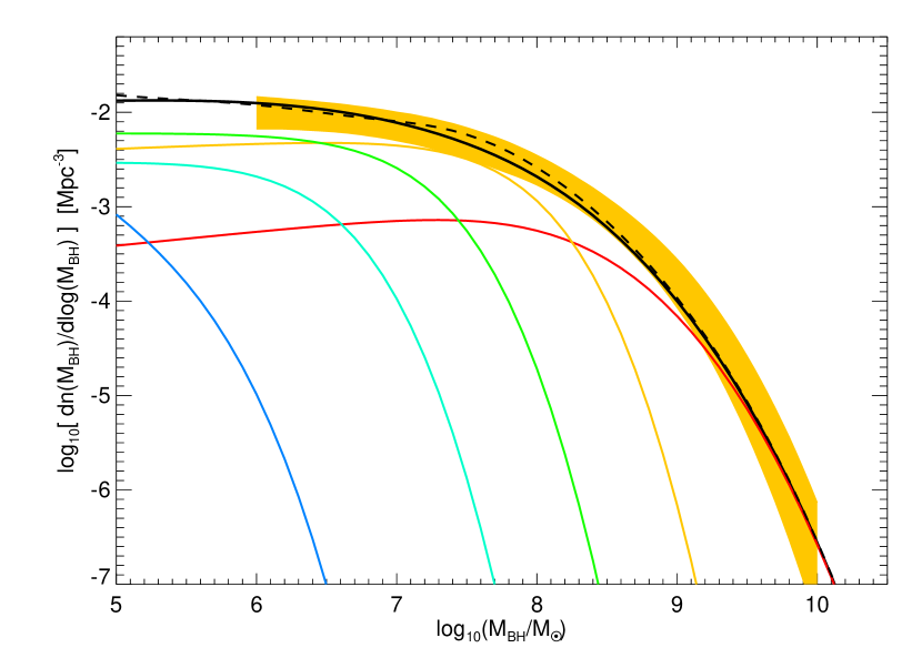
Figure 1.— Inferred black hole mass function from the morphological mass functions of Marzke et al. (1994a, b); Kochanek et al. (2001); Bell et al. (2003), with the typical bulk-disk decompositions of Aller & Richstone (2002); Shen et al. (2003); Hunt et al. (2004a); Tasca & White (2005) and $M_{\rm BH}-M_{\rm bulge}$ relation of Marconi & Hunt (2003); Robertson et al. (2005) or, equivalently, $M_{\rm BH}-\sigma$ relation from Tremaine et al. (2002). The mass function from E (red), S0 (yellow), Sa/b (green), Sc/d (cyan), Sm/Im (blue; assumes a maximal bulge B/T$=0.02$), and all types (black solid) are shown, and compared to the $1\sigma$ range of the inferred mass function from Marconi et al. (2004), based on the observations of Marzke et al. (1994a); Kochanek et al. (2001); Nakamura et al. (2003); Bernardi et al. (2003); Sheth et al. (2003) (yellow shaded range). The results adopting the modified $M_{\rm BH}-\sigma$ relation suggested in § 5 are also shown (black dashed).

In Figure 1, we show the resulting BHMF, calculated individually for each morphological category of E (red), S0 (yellow), Sa/b (green), Sc/d (cyan), and Sm/Im (blue). The cumulative BHMF obtained by summing these contributions is shown as the black line. For comparison, the BHMF determined in Marconi et al. (2004) is shown as the shaded yellow range, which also agrees with other measurements of the BHMF by e.g. Salucci et al. (1999); Marconi & Salvati (2002); Yu & Tremaine (2002); Ferrarese (2002); Aller & Richstone (2002); Shankar et al. (2004). That the agreement with our estimate is good suggests that our adopted conversions and decompositions are reasonable. For the Sm/Im case, we have assumed a maximal $B/T=0.02$, only a factor of $\approx 3$ below that of the Sc/d galaxies, and it is apparent that the contribution to the integrated BHMF and number density at any mass of interest is negligible. Therefore, we ignore these galaxies in our subsequent analysis, as their $B/T$ is in detail quite uncertain (if it is non-zero at all).

We now have the observed BHMF, with the corresponding gas fraction, bulge size and velocity dispersion, and disk mass and size for each system. Our calculations above then allow us to estimate the rates, duty cycles, and lifetimes of Seyfert activity fueled by the quiescent accretion of cold gas, and the corresponding Seyfert luminosity function.

For each black hole (i.e. each point in the joint PDF of $M_{\rm BH},\ \sigma,\ f_{\rm gas},\ M_{\rm d}$, and host galaxy type), we convolve the black hole distribution with the duty cycle as a function of these properties. In other words, the observed luminosity function is given by

$$\phi(L)\equiv\frac{{\rm d}\Phi(L)}{{\rm d}\log{L}}=\int\frac{{\rm d}f}{{\rm d}\log{L}}(\bar{x})\,{\rm d}n(\bar{x})$$ (90)

where $\bar{x}=(M_{\rm BH},\,f_{\rm gas},\,\sigma,\,M_{\rm d})$, for example. Again, we have $L\propto\dot{m}$ so ${\rm d}\log{L}={\rm d}\log{\dot{m}}$. Given our blast wave solution for ${\rm d}f/{\rm d}\log{\dot{m}}$, the distribution of host galaxy properties then completely determines the predicted Seyfert luminosity function (insofar as it is attributable to this fueling mechanism).

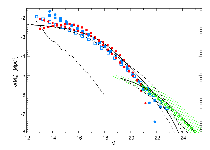
Figure 2.— Predicted intrinsic Seyfert luminosity function from our blast wave model. Solid black line extending to the upper left shows the prediction assuming $\eta_{L}=18/31$ as calculated in § 2, dashed and dotted lines show the predictions varying $\eta_{L}$ to $\eta_{L}=1/2$ and $\eta_{L}=1$, respectively. The observed SDSS Seyfert luminosity function from narrow-line H$\alpha$ (i.e. isotropic, intrinsic luminosity function) from Hao et al. (2005) is shown (blue), with both a double-power law (squares) and Schechter function (circles) fit to the observations, converted to intrinsic $B$-band using the corrections derived by the authors (filled) and a constant conversion following Mulchaey et al. (1994); Elvis et al. (1994) (open), each over the observed range. The luminosity function from [OII] measurements is shown in the same style (red). Green diamonds and shaded region show the quasar luminosity function extrapolated to $z=0$ from Ueda et al. (2003) and Richards et al. (2005), respectively, with predicted contribution of merger-driven, spheroid-forming quasar activity from Hopkins et al. (2006a) (solid black line in lower right for bolometric corrections of Marconi et al. (2004), dashed a constant $L=17\,L_{B}$). Contribution from stellar winds is shown (dot-dashed) as estimated in § 8. The expected Seyfert luminosity function from accretion of cold gas and our model for feedback-driven, self-regulated evolution dominates and agrees well with the observed luminosity function from $-15\lesssim M_{B}\lesssim-23$, with relatively weak dependence on the theoretical uncertainties for all but the brightest systems.

In Figure 2 we show the Seyfert luminosity function predicted by our blast wave model and the assumption of fueling by the accretion of molecular clouds. Our prediction, in terms of the bolometric luminosity, is converted to a $B$-band luminosity function using bolometric corrections following Marconi et al. (2004), based on optical through hard X-ray observations (e.g., Elvis et al., 1994; George et al., 1998; Vanden Berk et al., 2001; Perola et al., 2002; Telfer et al., 2002; Ueda et al., 2003; Vignali et al., 2003), with an X-ray reflection component generated by the PEXRAV model (Magdziarz & Zdziarski, 1995), and the appropriate Jacobian factors inserted. We have not calculated the effects of obscuration, and thus the luminosity function plotted is in terms of the intrinsic $B$-band luminosity, not necessarily that observed.

For comparison, we plot the local ($0<z<0.15$) AGN luminosity functions from the SDSS, determined in Hao et al. (2005). The luminosity function estimated from H$\alpha$ emission-line measurements is shown as blue points, over the luminosity range for which measurements exist. We show both the best-fit Schechter function (circles) and double power-law (squares) to the data. We convert to the $B$-band following Hao et al. (2005), based on the color corrections determined therein and from Schneider et al. (e.g., 2002, 2003). To show the effects of different bolometric corrections, the open squares adopt the constant bolometric corrections of Mulchaey et al. (1994); Elvis et al. (1994). In either case, the authors note that this gives agreement with previous, but much shallower and more poorly constrained $B$-band AGN luminosity function measurements from Huchra & Burg (1992) and Ulvestad & Ho (2001). The luminosity function shown is determined from the H$\alpha$ narrow-line component, and is thus expected to be isotropic to Seyfert 1 and Seyfert 2 galaxies, i.e. tracing the intrinsic luminosity which our prediction shows.

We also show (red points) the luminosity function determined from [O II] emission-line measurements, which is also expected to trace the intrinsic luminosity, with circles and squares again showing the best-fit Schechter and double power-law functions over the observed range. The correction to the $B$-band follows Mulchaey et al. (1994); Elvis et al. (1994), and gives agreement with the H$\alpha$ determination over the range where the observations are most well-constrained. However, this does illustrate the potential importance of systematic effects, especially at low luminosities.

There is some ambiguity about the proper value of $\eta_{L}$ (recall $L\propto t^{-\eta_{L}}$) to use in blast wave solution for the evolution of the quasar light curve, depending on the exact derivation from § 2. The solid line in the figure shows our prediction for $\eta_{L}=18/31$, the exact solution to the perturbative accretion flow in a medium with $\gamma=5/3$ and $k_{\rho}=0$ (i.e. assuming no strong density gradients in the cloud). Allowing for variation in $\gamma$ and $k_{\rho}$ in a reasonable range, assuming the black hole feedback immediately decouples from the blast wave once the blowout begins, or using instead e.g. the estimate of the Bondi rate at $R_{\rm BH}$ in the interior of the blast wave yield $\eta_{L}$ in the range $1/2\lesssim\eta_{L}\lesssim 3/2$. Therefore, we show in the figure our prediction for $\eta_{L}=1/2$ (dashed) and $\eta_{L}=1$ (dotted).

The primary change is at high accretion rates – a lower $\eta_{L}$ means a slower decay in the accretion rate, giving more time at high accretion rates and high luminosities (see § 4.5). However, the difference in the predictions is small even at the highest luminosities, and completely negligible at $M_{B}\gtrsim-20$, where the observations are most well-constrained. In fact, the systematic uncertainty from different bolometric corrections (compare e.g. the open and closed observational points) is a larger source of error at all luminosities than this theoretical uncertainty in the exact blast wave evolution.

We also show for comparison the extrapolation of the SDSS-2dF quasar luminosity function from Richards et al. (2005) to $z=0$ (see also Boyle et al., 2000), with the $1\sigma$ range indicated as the green shaded range at high luminosities. Similarly, we show the extrapolation of the Ueda et al. (2003) hard X-ray luminosity function to $z=0$ as open green diamonds over the same luminosity interval, converted to a $B$-band luminosity function again using the bolometric corrections of Marconi et al. (2004). We show the corresponding (lower right) predictions from the model for merger-induced quasar activity of Hopkins et al. (2006a, c), which reproduces the observed bright quasar luminosity functions over a wide range of redshifts and luminosities, as the solid black line (adopting the bolometric corrections of Marconi et al., 2004) and dashed black line (adopting the corrections of Elvis et al., 1994).

The difference in shape between the quasar and Seyfert luminosity functions is related to several effects. First, the mass function of black holes and, correspondingly, the systems “driving” accretion is different (the merger mass function for quasars, and the blue galaxy mass function for Seyferts). Second, our feedback-driven model gives slightly different decay solutions for both. We explicitly calculate different timescales for decay in the two regimes in § 3, and owing to changes in the external mass profile and initial energy injection, the profile for the decay (i.e. faint-end slope) will be different. Essentially, in more violent quasar systems, the feedback drives the system to lower luminosities more quickly, resulting in a shallower faint-end slope of the luminosity function (Hopkins et al., 2006c).

The agreement between the predicted and observed luminosity functions is good over a wide range of luminosities, from $M_{B}\gtrsim-14$ to $M_{B}\lesssim-22$, and further if we consider the predicted quasar contribution from other fueling mechanisms. At the lowest luminosities $M_{B}\gtrsim-14$, our prediction agrees with the [O II] determinations, but underpredicts the luminosity function estimated from H$\alpha$ measurements. However, there are several sources of uncertainty at low luminosities. A detailed comparison of the Seyfert 1 and Seyfert 2 H$\alpha$, [O II], and [O III] luminosity functions in Hao et al. (2005), including a comparison between different selection criteria from Kewley et al. (2001) and Kauffmann et al. (2003a), suggests that there may be significant contamination by star formation at these luminosities in H$\alpha$, resulting in a significantly higher estimate (note that we compare with the stricter AGN cut the authors adopt, although contamination is still possible).

Additionally, measurement errors and bin-to-bin variation are significant at these luminosities, $\sim 0.3\,$dex. Moreover, the luminosity function must turn over strongly near these luminosities. Although the Seyfert number density implied by integrating the observed luminosity function over the observed range implies that approximately $20\%$ of galaxies host a Seyfert in this luminosity interval (an observation necessarily reproduced by our modeling since our predicted luminosity and mass functions agree with those observed), extrapolating this luminosity function only $1.5$ magnitudes fainter would imply that there are more Seyferts than there are galaxies. Finally, alternative fueling mechanisms such as stellar winds may become important at these lowest luminosities, a point discussed in § 8.

4.4. Contribution of Different Morphological Types

Our analysis enables us to decompose the contributions to the AGN luminosity function from different galaxy types. At the brightest end, above the break in the extrapolated quasar luminosity function, the systems are traditional “bright quasars”, which may be entering the blowout phase in the final stages of a galaxy merger, expelling the remaining gas in a newly-formed elliptical galaxy, a model described in detail by Hopkins et al. (2005a-e; 2006a-e). The volume density of these objects is very low, $\ll 10^{-7}\,{\rm Mpc^{-3}}$, and thus while they may dominate the bright AGN population at high redshifts they will not be observed locally even in large surveys such as the SDSS.

At luminosities below the break in the extrapolated quasar luminosity function and at the brightest end of the AGN luminosity function, there is a substantial contribution from black holes relaxing after the blowout stage in their host and black hole-forming mergers. These follow a similar decay to the blast wave solution described above and in Hopkins et al. (2006b) (both analytically and from simulations of mergers) for the specific case of post-merger blowout ($\dot{m}\propto t^{-2}$), a steeper typical decay than for Seyferts. These host galaxies rapidly redden and evidence of disturbance fades quickly, and they will be seen as relatively normal ellipticals with large black holes at moderate to low accretion rates, with possible evidence for recent ($\lesssim\,$Gyr) merger or star formation activity. This population, with precisely these properties and a similar fractional contribution to that we predict at the bright end of the local AGN luminosity function, is well known observationally (e.g., Kauffmann et al., 2003a; Sánchez & González-Serrano, 2003; Sánchez et al., 2004), even in cases where the AGN dominates the observed spectrum (Vanden Berk et al., 2005).

The bulk of the luminosity range from $-15>M_{B}>-20$ is dominated by late-type systems at moderate to high accretion rates, fueled by the accretion of cold gas. At the brightest luminosities, there is some contribution to the AGN luminosity function from relaxing ellipticals, but at lower luminosities (as is evident from the predicted post-merger AGN luminosity function prediction in Figure 2) this contribution becomes small. Ellipticals do not significantly contribute to the AGN luminosity function determined by this fueling mechanism, as they do not have a supply of cold gas. The luminosity function from this mode of fueling is mainly determined by systems of intermediate mass ($M_{\rm BH}\sim 10^{7}\,M_{\sun}$) in Sa/b systems and to a slightly lesser extent (owing to their lower gas content) by S0s. Sc/d galaxies may not be an insignificant contribution to the Seyfert luminosity function, but they do not dominate owing to both their lower characteristic black hole masses (by a factor $\sim 10-30$) and lower number density (by a factor $\sim 2$) compared to both Sa/b and S0 systems. In general, systems with small bulges and black holes $\lesssim 10^{6}\,M_{\sun}$ (see § 4.1) may only contribute significantly at the lowest luminosities $M_{B}\gtrsim-15$. As discussed in § 4.3 above, Sm/Im galaxies have such low black hole masses (if any) that they contribute negligibly.

This distribution of AGN hosts for this luminosity interval is consistent with observations (Kauffmann et al., 2003a; Sánchez et al., 2004; Best et al., 2005), specifically those of e.g. Dong & De Robertis (2005) who find that Sa/b and S0 systems make up most of the low-moderate luminosity contribution to the Seyfert luminosity function, with a relatively small contribution from Sc/d systems. Similarly, the range of masses and host galaxy types for which large $\dot{m}\gtrsim 0.1$ accretion rates are predicted agrees with observational estimates suggesting that present-day black hole growth (in the sense of the population of high-Eddington ratio objects) is dominated by late-type, seemingly normal systems with black hole masses in the range given above (Cowie et al., 1996; Steffen et al., 2003; Barger et al., 2003; Ueda et al., 2003; Heckman et al., 2004), as discussed in more detail in § 4.5.

At the lowest luminosities, there is a substantial contribution from low-Eddington ratio accretion in late-type systems, but also from relaxed ellipticals at low accretion rates. Fueling by stellar winds, either from young star clusters in systems which still have cold gas or smaller contributions from aging stellar populations in old bulges has long been recognized as a significant fuel source for accretion (e.g., Shull, 1983; Mathews, 1983; David et al., 1987), however the high velocities of these winds yield relatively low Bondi rates, and a wide variety of observations further show that such systems tend to be accreting at rates significantly below the Bondi estimate (Fabian & Canizares, 1988; Blandford & Begelman, 1999; Di Matteo et al., 2000; Narayan et al., 2000; Quataert & Gruzinov, 2000; Di Matteo et al., 2001; Loewenstein et al., 2001; Bower et al., 2003; Pellegrini, 2005).

Nevertheless, these can provide a significant contribution to the lowest-luminosity systems, and many “dead” ellipticals with accretion rates $\dot{m}\sim 10^{-6}-10^{-4}$ are expected and observed (e.g., Ho, 2002; Heckman et al., 2004; Marchesini et al., 2004; Jester, 2005; Pellegrini, 2005). These may also be fueled by mechanisms other than stellar winds or the accretion of hot (virialized) gas, but this seems to account for most of the objects here, as calculated in § 8, especially if one accounts for feedback removing some of the accreted mass in a steady-state solution (Soria et al., 2005b). We show the prediction for the contribution from stellar wind and hot gas fueling in Figure 2 as the dot-dashed line, which demonstrates the lower accretion rates of such systems, but the narrower luminosity range results in a steeper stellar-wind induced luminosity function which becomes important at the lowest luminosities.

4.5. Distribution of Eddington Ratios

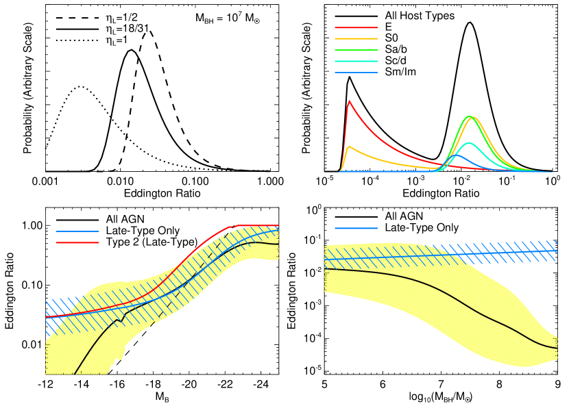
Figure 3.— Upper left: Predicted distribution of Eddington ratios $\dot{m}\equiv\dot{M}/\dot{M}_{\rm Edd}$, for late-type active (i.e. in some stage of “blowout”) systems with $M_{\rm BH}=10^{7}\,M_{\sun}$, predicted by our blowout model in Equation (86). Results for different rates of accretion rate decay $\eta_{L}$ are shown, as labeled (note that the vertical axis is a linear scale). Upper right: Cumulative Eddington ratio distribution in active systems (systems having a high-accretion rate event in a Hubble time) with $M_{B}\lesssim-12$, as a function of morphological type, with late type Eddington ratios estimated as above and the E/S0 contribution from post-spheroid forming merger decay estimated following Hopkins et al. (2006a, b, c). Lower left: Mean Eddington ratio and rms dispersion (shaded range) as a function of $M_{B}$ from the Eddington ratio PDFs and predicted Seyfert luminosity function in Figure 2, for all AGN (black, with yellow dispersion), AGN in late-type hosts (blue; modeled herein), and Type 2 AGN in late-type hosts (red; dispersion not shown for clarity but similar to that of all late-type AGN). Note that this does not imply higher Eddington ratios for Type 2 AGN as a whole, as the luminosity-dependence of the Type 2 fraction is important for such a statistic (see Figure 9). Dashed line shows the expectation if $M_{\rm BH}=3\times 10^{7}\,M_{\sun}$= constant (i.e. implying the luminosity function is dominated by differences in Eddington ratio). Lower right: Mean Eddington ratio and rms dispersion, in the same style, as a function of $M_{\rm BH}$.

From the evolution of the accretion rate in our blast wave solution, we can predict the accretion rate distribution as a function of e.g. black hole mass, luminosity, and host galaxy properties. Figure 3 shows (upper left) the predicted Eddington ratio distribution ${\rm d}f/{\rm d}\log{\dot{m}}$ for “active” (i.e. in some stage of blowout) late-type systems determined in Equation (86), with the appropriate exponential cutoff at low $\dot{m}$ (such that $\int{\rm d}f=1$). We show this for $M_{\rm BH}=10^{7}\,M_{\sun}$, where $\tau_{\ast}\approx 1$ (as determined in Equation [3.2]) and typical of the black holes which dominate the Seyfert luminosity function, but our calculation in § 4.2 demonstrates that this distribution depends only weakly on $M_{\rm BH}$ in late-type systems.

We show results for three values of $\eta_{L}$: $\eta_{L}=1/2$ (dotted), $\eta_{L}=18/31$ (solid), and $\eta_{L}=1$ (dashed). Because $L\propto t^{-\eta_{L}}$, larger values of $\eta_{L}$ correspond to a more rapid falloff in the accretion rate and therefore broader Eddington ratio distributions extending to lower accretion rates. In what follows, we adopt $\eta_{L}=18/31$, and a different $\eta_{L}$ will not change the trends in Eddington ratio which we find but will systematically shift the typical Eddington ratios as shown in the figure. As is clear from comparison with Figure 2, the exact choice of $\eta_{L}$ has little effect on our predicted Seyfert luminosity function, within the reasonable range of $\eta_{L}$ predicted by our blast wave model, $1/2\leq\eta_{L}\leq 3/2$. However, $\eta_{L}$ dominates the systematic uncertainty in the estimated Eddington ratio distribution.

Figure 3 also shows (upper right) the predicted cumulative Eddington ratio distribution as a function of host galaxy morphology. Here, the small differences in the Eddington ratio distribution among late-type galaxies are caused by the weak dependence of $\tau_{\ast}$ and the duty cycle on host galaxy properties ($\sigma$ and $f_{\rm gas}$). The Eddington ratio distribution of ellipticals and inactive S0s is estimated from the predicted formation times and blast wave decay of merger-induced quasar activity (Hopkins et al., 2006a, b, c). The “cumulative” Eddington ratio is, in general, ill-defined, and here we plot the distribution in active (i.e. with an event in $t_{H}$) systems with $M_{B}\lesssim-12$.

The lower left panel of Figure 3 shows the (logarithmic) mean Eddington ratio and rms dispersion (shaded ranges) as a function of $M_{B}$ from the Eddington ratio PDFs above and predicted Seyfert luminosity function in Figure 2. We show this for all AGN (black, with yellow shaded range), AGN in late-type hosts as modeled herein (blue), and Type 2 AGN in late-type hosts as calculated in § 6.1 below (red; dispersion not shown for clarity but similar to that of all late-type AGN). The $B$-band magnitude $M_{B}$ represents the intrinsic magnitude as in Figure 2, and does not account for extinction. In the lower right panel of the Figure, we show the same quantity as a function of black hole mass.

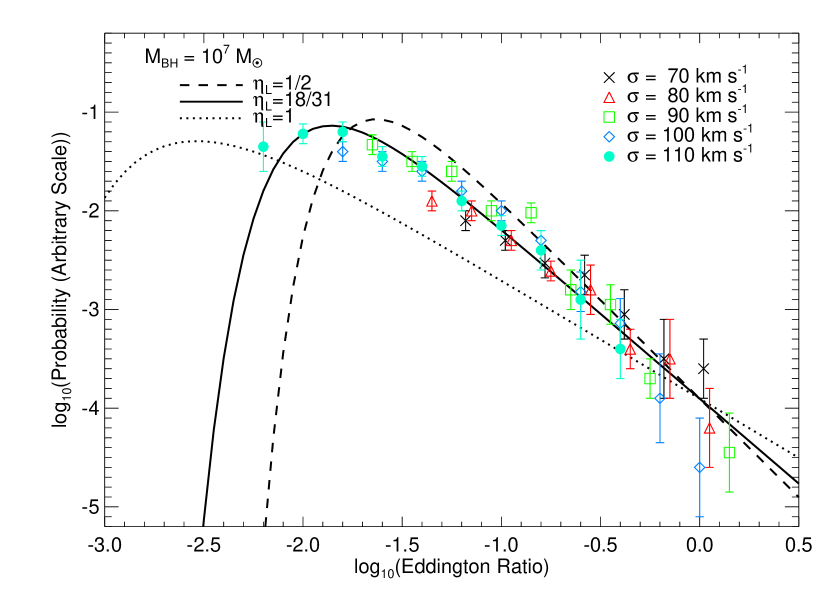
Figure 4.— Predicted Eddington ratio distribution of active Seyferts from our blast wave model in § 2 and for estimated duty cycles in § 4.2, as in Figure 3 (upper left), for our exact solution $\eta_{L}=18/31$ and the range $\eta_{L}=1/2,\,1$ as labeled, for black holes with $M_{\rm BH}=10^{7}\,M_{\sun}$ (although this depends only weakly on $M_{\rm BH}$). The observed accretion rate distribution from Yu et al. (2005) is plotted for each of several values of $\sigma$ as labeled, corresponding to $M_{\rm BH}\approx 2\times 10^{6}-2\times 10^{7}\,M_{\sun}$. Both the power law-trend at high $\dot{m}$ (dependent on the feedback-regulated light curve decay) and flattening/turnover at low $\dot{m}$ (dependent on excitation rates and duty cycles) in the observed distribution agree very well with the predictions of our model ($\chi^{2}/\nu=0.6$), whereas models without feedback-driven self regulation of the accretion rate produce much flatter distributions.

Figure 4 shows our predicted Eddington ratio distribution, as in the upper left panel of Figure 3 (but in log-log). Recall that this shows our prediction of ${\rm d}f/{\rm d}\log{\dot{m}}$, the fraction of objects per logarithmic interval in $\dot{m}$. We compare our results with those measured in Yu et al. (2005) from a sample of $\gtrsim 20,000$ local SDSS AGN (points), from estimates of [OIII] luminosities and black hole masses inferred from measurements of $\sigma$. We show the observations for five values of $\sigma$, from $\sigma=70-110\,{\rm km\,s^{-1}}$ (binned by $0.05$ dex in $\log{\sigma}$). We show this range of $\sigma$ because it corresponds approximately to $M_{\rm BH}=2\times 10^{6}-2\times 10^{7}\,M_{\sun}$, appropriate for comparison with our predictions for $M_{\rm BH}=10^{7}\,M_{\sun}$. Furthermore, at larger $\sigma$, there is a significant contribution from “dead” ellipticals (as seen in e.g. the black hole mass function of Figure 1 or Eddington ratio as a function of $M_{\rm BH}$ in Figure 3), and while we can predict the combined Eddington ratio distribution at these $\sigma$ by combining our predictions with those of Hopkins et al. (2006a, b), the relation to our blast wave model and physical interpretation is less direct.

The agreement between our predicted Eddington ratio distribution and the observations is good ($\chi^{2}/\nu=0.6$ for the comparison with the $M_{\rm BH}=10^{7}\,M_{\sun}$, i.e. $\sigma\approx 100\,{\rm km\,s^{-1}}$ data), over the observed range. The agreement for $1/2\leq\eta_{L}\leq 5/6$ is less good, but still acceptable ($\chi^{2}/\nu\sim 1.5-2.0$). Note that we follow Yu et al. (2005) and exclude the lowest Eddington ratio bin for each $\sigma$ owing to significant incompleteness. In order to compare with their observations, we have convolved our prediction with the distribution of [OIII] luminosities (i.e. allowed for a small dispersion in bolometric correction), which is why our prediction is non-zero (although small) above an Eddington ratio of unity. The predicted Eddington ratio distribution in this mass range depends only weakly on $\sigma$, evident in e.g. our Equation (3.2) and in Figure 3, and therefore the observations over this entire range in $\sigma$ all agree with our prediction in a nearly self-similar manner.

That the observed Yu et al. (2005) $\dot{m}$ distributions agree with our exact blast wave solution with $\eta_{L}=18/31$ and reasonably well with e.g. the range of solutions $1/2\leq\eta_{L}\leq 5/6$ is somewhat surprising. The slope this implies (i.e. logarithmic slope of ${\rm d}n/{\rm d}\log{\dot{m}}$) of $-1/\eta_{L}=-31/18$ is substantially different from the slope of $\approx-0.8$ fitted to the low-$\dot{m}$ behavior of the $\dot{m}$ distributions by the authors, which would imply $\eta_{L}\approx 1.26\pm 0.1$. The authors use this fit to argue for a self-similar quiescent disk evolution model to explain the late-time $L\propto t^{-\eta_{L}}$ behavior. However, this fit from Yu et al. (2005) is derived primarily from the low-$\dot{m}$ behavior of their $\sigma\approx 200\,{\rm km\,s^{-1}}$ objects, which we have noted (following numerous observational studies) are a different population, dominated by ellipticals decaying from larger accretion rates or fueled by e.g. stellar winds and diffuse hot gas (e.g., Kauffmann et al., 2003a; Pellegrini, 2005). Furthermore, the authors acknowledge that this does not provide a good fit to objects with larger $\sigma$, which is surprising since these objects are otherwise observed to be a similar AGN population to those with $\sigma\approx 200\,{\rm km\,s^{-1}}$ (i.e. both are dominated by early-type systems). The authors also acknowledge that this model for the activity predicts that the active black holes will be observed at masses substantially below their final ($M_{\rm BH}-\sigma$ relation) masses, by about $1\,$dex, whereas the observations (e.g., Barth et al., 2005) suggest the opposite trend. In § 5 we demonstrate that our model predicts this observed tendency rather than smaller black hole masses.

Additionally, the model fitted by Yu et al. (2005) does not provide a good match to the high-$\dot{m}$ distributions, even for those values of $\sigma$ for which the overall fit is most acceptable, giving e.g. typical $\chi^{2}/\nu\sim 4-6$ for $\sigma\sim 100-200\,{\rm km\,s^{-1}}$ (at $\dot{m}\gtrsim 10^{-2}$). Over the entire observed range, our model provides an improved fit, $\chi^{2}/\nu\approx 0.6$ compared to $\chi^{2}/\nu\approx 1.6$ from the fits of Yu et al. (2005); alternatively, $\Delta\chi^{2}\approx 11.0$ for e.g. $\sigma=110\,{\rm km\,s^{-1}}$. These arguments suggest that while the self-similar quiescent disk evolution discussed in Yu et al. (2005) may be important for some range of early-type systems at low accretion rates, the observations in the range of black hole masses shown in Figure 4 are better explained by our model for feedback-driven blast wave evolution.

The turnover at low-$\dot{m}$ in the Eddington ratio distribution is, for any power-law distribution of accretion rates, set entirely by the duty cycle at high $\dot{m}$. In our language, for a given slope $\eta_{L}$, this turnover occurs at a value $\dot{m}_{\rm min}$ determined by Equation (88) as a function of the duty cycle (i.e. lifetime and rate of activation) at high $\dot{m}$. There is some uncertainty in the exact normalization of this turnover, as our theoretical prediction depends on scaling arguments and the detailed numerical prefactors are sensitive to the local kinematics near the black hole. Therefore, our prediction for the location of the turnover is more uncertain than our prediction of $\eta_{L}$.

Currently, the observations do not resolve the turnover. Doing so would constrain the duty cycle as a function of $\dot{m}$; for example, the difference between a sharp turnover as we have assumed and a shallow (e.g. symmetric power-law) turnover for the $\dot{m}_{\rm min}$ of our $\eta_{L}=18/31$ prediction amounts to a factor of $\sim 2$ change in the duty cycle $\delta_{0}$. Therefore, observations of the shape of the accretion rate distribution at a given $\sigma$, probing only moderately fainter luminosities than Yu et al. (2005), can constrain this quantity without the large systematic uncertainties inherent in determining the normalization of the distribution when the turnover is not resolved. We note, however, that at least the flattening of this distribution at low $\dot{m}$ is resolved by the observations of Yu et al. (2005) – if our prediction were simplified to a pure power-law, it would overpredict by $\sim 3-6\sigma$ each of the lowest four $\dot{m}$ observations plotted.

Figure 5.— Left: Mean Eddington ratio as a function of black hole mass from Figure 3, compared to estimates from the observations of Heckman et al. (2004) (squares). The point at $M_{\rm BH}\approx 3\times 10^{6}\,M_{\rm sun}$ shows the absolute systematic uncertainty in the mean Eddington ratio distribution from fitting to the (high Eddington ratio only) distributions of Heckman et al. (2004), subsequent points show the relative uncertainty in the trend of Eddington ratio vs. $M_{\rm BH}$. The observed trend of decreasing Eddington ratios with $M_{\rm BH}$ is reproduced, as larger-$M_{\rm BH}$ populations are increasingly dominated by large spheroids without cold gas supplies for stochastic accretion. Right: Tentative Eddington ratio distribution from Figure 3 (upper left), summed over all morphological types, compared to the observationally estimated Eddington ratio distribution from Marchesini et al. (2004) (histogram). Note, however, that the vertical axis here is linearly scaled, and the predicted bimodality can easily be erased by e.g. different values of $\eta_{L}$.

Although incompleteness in the lowest-$\dot{m}$ bin at each $\sigma$ may be significant, the observations appear to favor the turnover in the Eddington ratio distribution moving to larger $\dot{m}$ at lower $\sigma$, an expectation broadly consistent with our result in the lower-left panel of Figure 3. Figure 5 shows our prediction for the mean Eddington ratio as a function of black hole mass from Figure 3, compared to the estimates of Heckman et al. (2004) (squares). Neither the observations of Heckman et al. (2004) nor those of Yu et al. (2005) resolve the turnover in accretion rate distributions at low-$\dot{m}$, and therefore cannot determine a “mean” accretion rate in a proper sense. Therefore, we instead consider the cumulative distribution of accretion rates from the observations for $M_{\rm BH}\approx 3\times 10^{6}\,M_{\rm sun}$, and fit this to a distribution of Eddington ratios similar to our prediction in Figure 4 above, but allowing both the slope and duty cycle to vary freely. From these fits, then, we can constrain the peak and mean of the Eddington ratio distribution. The vertical error bars of the point at $M_{\rm BH}=3\times 10^{6}\,M_{\rm sun}$ in Figure 5 show the $1\sigma$ allowed range from these fits, and reflect the systematic uncertainty in the absolute value of the mean accretion rates at a given $M_{\rm BH}$ or $\sigma$ determined observationally.

While the mean Eddington ratios are not well-determined observationally, the trend of Eddington ratio with mass is more well-constrained. Using the best-fit absolute normalization from the fit to the $M_{\rm BH}=3\times 10^{6}\,M_{\rm sun}$ data, we show the expected mean Eddington ratio as a function of $M_{\rm BH}$ at $M_{\rm BH}=10^{7},\ 3\times 10^{7},\ 10^{8},\ 3\times 10^{8},\ {\rm and}\ 10^{9}\,M_{\sun}$ from the observed trends in Heckman et al. (2004) (see their Figure 3). Here, the vertical error bars represent the relative error in Eddington ratio as a function of mass. Thus, the typical mean Eddington ratios do agree with our predictions, but the uncertainties are large because the downturn of the $\dot{m}$ distribution is not measured observationally. However, the trend of mean Eddington ratio with black hole mass is reasonably well-constrained, and agrees with our predictions for black hole masses $M_{\rm BH}=3\times 10^{6}-10^{9}\,M_{\sun}$.

The trend arises because for higher black hole masses, the population is increasingly dominated by ellipticals which do not have a supply of cold gas. These systems are presumably either fading from earlier bright quasar activity or accreting in a quasi-steady state from virialized hot gas or stellar mass loss, at accretion rates well below those of late-type Seyferts. Furthermore, the mean age of ellipticals may increase with mass, here calculated following the determination as a function of bulge and black hole mass in Hopkins et al. (2006b), further contributing to the trend of decreasing $\dot{m}$ with increasing $M_{\rm BH}$ even in pure elliptical systems.

From Figure 5, our modeling predicts that most of the black hole mass growth in the local Universe occurs in relatively low-$M_{\rm BH}$ systems with $M_{\rm BH}\lesssim 10^{7}\,M_{\sun}$, consistent with observations (Heckman et al., 2004). Of course, observations of quasars, compared to our predictions for the evolution of cloud-fueled activity in late-type galaxies in § 4.6, suggest that this is not true at higher redshifts, where more massive black holes are formed. Although this constitutes the low-redshift end of “cosmic downsizing” (e.g., Cowie et al., 1996) seen observationally in AGN and quasar evolution (Page et al., 1997; Miyaji et al., 2000, 2001; La Franca et al., 2002, 2005; Cowie et al., 2003; Ueda et al., 2003; Fiore et al., 2003; Hunt et al., 2004b; Cirasuolo et al., 2005; Hasinger, Miyaji, & Schmidt, 2005), our modeling does not imply that the local activity is fundamentally cosmological. The transition to lower black hole masses growing at lower redshifts through black hole growth via merger-driven quasar fueling is cosmological and traces galaxy downsizing (Hopkins et al., 2006b). But, the relatively high rates of accretion in late-type galaxies compared to higher-$M_{\rm BH}$ systems predicted here is more a function of the high-$M_{\rm BH}$ ellipticals fading with time, rather than any sudden “turning on” of the Seyfert population.

In Figure 5 we also compare our result for the total distribution of accretion rates across all morphological types from the upper right panel of Figure 3 (solid line) to that determined by Marchesini et al. (2004) (shaded histogram), which agrees with the estimates of e.g. Ho (2002); Jester (2005); Hopkins et al. (2005e) and extends to lower $\dot{m}$ than that of e.g. Yu et al. (2005) and includes inactive systems. The predicted Eddington ratio distribution is bimodal, with Seyferts comprising the majority of the high-$\dot{m}$ peak and relaxed ellipticals dominating at low $\dot{m}\sim 10^{-4}$ accretion rates. There is broad agreement, and the slight horizontal offset between the theory and measurements is within the systematic uncertainty of the observational estimate of $\dot{m}$.

While this agreement is suggestive, we caution that the predicted bimodal distribution is not firm. The vertical axis shows a linear scale, and, from Figure 4, a small change in our choice of $\eta_{L}$ or the duty cycle at high $\dot{m}$ (which determines the $\dot{m}_{\rm min}$ where the high-$\dot{m}$ distribution turns over) would broaden the distribution to $\lesssim 10^{-3}$, erasing the bimodality. Furthermore, our prediction depends on the Eddington ratio distribution of quiescent ellipticals, estimated from their accretion rate decay according to our blast wave model following mergers and simulations of merger-driven black hole growth (Hopkins et al., 2006a, c), but once these low accretion rates are attained, other processes may dominate the gas inflows and accretion, and thus our estimate may not be appropriate for this end of the distribution.

In the lower-left panel of Figure 3, we show our prediction (solid line) for the mean accretion rate as a function of luminosity, compared (dashed line) to the corresponding Eddington ratio for a black hole of mass $3\times 10^{7}\,M_{\sun}$ at each $M_{B}$ (i.e. approximately a logarithmic slope of $-1/2.5$). This slope is what would be expected if the observed luminosity function were purely an Eddington ratio sequence. Although the differences between our predicted distribution and that shown are important, the rough similarity between the two, at least for $M_{B}\gtrsim-20$, implies that the range of the observed luminosity function is dominated by differences in Eddington ratio, and not by different black hole masses at similar relative accretion rates. Since e.g. host galaxy mass and luminosity are correlated with black hole mass, we expect that these quantities will not be strongly correlated with the observed AGN luminosity, as a wide range of AGN luminosities can have a similar distribution in constituent black hole masses. This has been seen in observations of local AGN and quasars and their host galaxies (e.g., Bahcall et al., 1997; McLure et al., 1999; Hamilton et al., 2002; Woo & Urry, 2002; O’Dowd et al., 2002; Jahnke & Wisotzki, 2003; Hao et al., 2005; Vanden Berk et al., 2005).

Note that the prediction for the Type 2 Eddington ratios in this panel, while slightly above those of Type 1 objects at high luminosities, does not imply that we predict typically higher accretion rates in Type 2 Seyferts. Rather, as shown in § 6.1, our modeling indicates that Type 2 Seyferts are a small fraction of the population at these high luminosities, but a large (comparable) fraction at low luminosities. Therefore, our modeling predicts that the characteristic accretion rates of Seyfert 2s should be lower than those of Seyfert 1s. In general, the differences in Eddington ratio distributions between Type 1 and Type 2 systems is a more sensitive function of their characteristic luminosities and determined by e.g. the dependence of the Type 2 fraction on luminosity, than it is a difference between the two populations at a given luminosity. (This refers to intrinsic luminosity, as Type 2 systems will, by definition, be extinguished at some frequencies.)

4.6. Redshift Evolution of Seyfert Activity

Our estimate of the duty cycle as a function of $\dot{m}$ depends primarily on the gas fraction and $\sigma$, and the convolution to give a luminosity function depends on the black hole mass function in late-type galaxies. From the evolution of these quantities it is straightforward to determine the evolution in this luminosity function.

Because the mass gained in a “blowout” event is small (at most a factor $\sim 2$; see § 5.4), we determine the black hole mass function at each redshift of interest from the evolution of the late-type galaxy mass function, using the method of § 4.3. From the spectral-type separated mass functions of Fontana et al. (2004) determined up to $z=2$ from the K20 survey, we expect little evolution in the late-type mass function up to $z\sim 1$, and then a decrease in the number density of these galaxies. In detail, we trace this evolution up to $z=0.5$ using the $K$ and $J$-band luminosity functions of e.g. Feulner et al. (2003); Pozzetti et al. (2003); Dahlen et al. (2005). Normalizing the mass functions to be the same in the overlapping redshift interval $0.2<z<0.55$, we extend this with the morphologically classified spiral mass functions from Bundy et al. (2005) and Franceschini et al. (2006) up to $z=1.4$, and then repeat this with the Fontana et al. (2004) observations to infer the mass functions to $z=2$.

These estimates are roughly consistent with the $B$-band evolution in late-type luminosity functions which is more well-constrained (e.g., de Lapparent et al., 2004; Giallongo et al., 2005; Faber et al., 2005), measured evolution in the cumulative mass function (de Propris et al., 1999; Drory et al., 2004, 2005), and evolution in black hole mass functions from spheroid luminosity functions and integration of the continuity equations for AGN luminosity functions (Yu & Lu, 2004; Tamura et al., 2005). Given this, our approach appears to be reasonable, but the observations have large uncertainties. However, we find that there is little evolution in the Seyfert luminosity function in any case, and these uncertainties are not important.

We estimate the evolution in the typical gas fractions of disks by assuming that gas is consumed on a timescale related to star formation $t_{\rm SF}\sim 4-8$ Gyr, giving $f_{\rm gas}\sim\exp{(-t_{H}(z)/t_{\rm SF})}$, where $t_{H}(z)$ is the Hubble time at redshift $z$. We take $t_{\rm SF}\sim 6\,$Gyr, as this gives a Milky-Way like $f_{\rm gas}\sim 0.1$ at $z=0$. This prescription and characteristic timescale follow from observations (e.g., Kennicutt, 1998; Rownd & Young, 1999; Martin & Kennicutt, 2001), cosmological simulations (e.g., Springel & Hernquist, 2003; Hernquist & Springel, 2003; Nagamine et al., 2004, 2005a, 2005b), simulations of star formation rate evolution in isolated disk galaxies (Li et al., 2005a, b), and comparison of these simulations and the predictions for quasar activity with merger rates and merger luminosity functions (Hopkins et al., 2006e). As gas fractions increase, the event rate for cold gas accretion can increase, producing a higher duty cycle at large $\dot{m}$ from Equation (87). Although our choice for the evolution of the gas fraction is somewhat arbitrary, we find a sufficiently weak dependence that observational uncertainty is not significant.

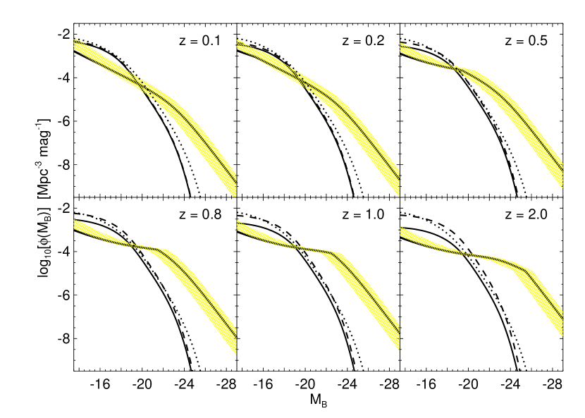
Figure 6.— Predicted Seyfert luminosity function owing to the stochastic fueling, at several redshifts (as labeled). The observed quasar luminosity function from Ueda et al. (2003) (black line with yellow shaded range) is shown, converted to $M_{B}$ as in Figure 2. The solid line (no shaded range) shows our prediction for the Seyfert luminosity function, determined from the evolution in late-type mass functions (de Propris et al., 1999; Drory et al., 2004, 2005; Fontana et al., 2004; de Lapparent et al., 2004; Bundy et al., 2005; Dahlen et al., 2005; Giallongo et al., 2005; Franceschini et al., 2006) and gas fractions (Kennicutt, 1998; Rownd & Young, 1999; Martin & Kennicutt, 2001; Springel & Hernquist, 2003; Li et al., 2005a, b). Dashed lines shows the “maximal evolution” (i.e. allowing gas fractions to increase with $z$ but not allowing any mass function decrease). Dotted lines show the $z=0$ prediction of Figure 2, i.e. no evolution. Regardless of our assumptions, the evolution in the luminosity function of systems fueled by quiescent, non-merger driven cold gas accretion is weak, and the quasar luminosity function at the redshifts of peak quasar activity (and quasar luminosity density) must be dominated by other fueling mechanisms.

Figure 6 shows our predicted Seyfert luminosity function (black lines with no shaded range) at various redshifts. The solid lines show the full prediction, accounting for both evolution in the late-type galaxy mass functions and the evolution in typical gas fractions of disk galaxies. The dashed line shows an estimate of “maximal evolution,” i.e. allowing the gas fraction to increase with redshift, but not allowing any decrease in the mass functions. The dotted line shows the $z=0$ prediction from Figure 2 at each redshift – i.e., no evolution.

For comparison, at each redshift, we show the fitted quasar luminosity function of Ueda et al. (2003) (black solid line with yellow range showing the uncertainty owing to different bolometric corrections), converted to $M_{B}$ as in Figure 2. The “low” ($0.2\leq z\leq 1$) redshift behavior of this luminosity function has also been compared with the luminosity functions of e.g. Richards et al. (2005); Hasinger, Miyaji, & Schmidt (2005) which have more objects at these redshifts, and they give consistent results. Alternatively, we could plot the expectation for merger-driven quasar activity calculated from the models and simulations of quasars in mergers from Hopkins et al. (2005a-e; 2006a-e), which is essentially identical to the plotted quasar luminosity functions.

From Figure 6 we see that the quasar luminosity function evolves rapidly, while our predicted Seyfert luminosity function hardly evolves even out to $z=2$. While our estimates of the evolution of e.g. gas fractions and late-type mass functions are uncertain, the similarity (relative to the evolution in the quasar luminosity function) of the expected evolution, no evolution, and maximal evolution cases means that unless an extreme model for late-type galaxy evolution were adopted (at odds with the observations), there would be essentially no difference in the predicted evolution of this luminosity function. Thus, these observational errors are not a significant source of theoretical uncertainty for the key conclusions from Figure 6.

From the figure, it appears that our prediction may be systematically high, by about a factor of $\sim 2$, at the lowest luminosities, which is possible, given the uncertainties in our estimate of the duty cycle. If the normalization at these luminosities is matched to the extrapolated faint end of the quasar luminosity function, then it implies an even smaller contribution from this activity at these redshifts. However, it is important to note that the faint end quasar luminosity function plotted here is extrapolated below the observations at the higher redshifts, and may be incomplete at the lowest $M_{B}\gtrsim-18$ luminosities, corresponding to or slightly below the faintest bins in even the deep luminosity functions of e.g. Ueda et al. (2003); Hasinger, Miyaji, & Schmidt (2005); La Franca et al. (2005) at low ($z\lesssim 1$) redshifts.

For local, $z=0$ AGN, the contribution from stochastic cold gas accretion dominates the luminosity function up to $M_{B}\approx-22$, near the traditional division between Seyfert and quasar activity (see Figure 2). However, above $z\sim 0.1$, this shifts to lower luminosity $M_{B}\approx-20$, and the relative contribution at higher luminosities steadily decreases. This luminosity function does still represent a significant contribution to the faint end (i.e. below the “break”) of the quasar luminosity function up to $z\sim 0.5$. However, by $z=1$, the “Seyfert” (i.e. our predicted) contribution to the quasar luminosity function is only significant at about $4-5$ magnitudes (i.e. two orders of magnitude in luminosity) below the break, and by $z=2$ only important about 7 magnitudes, or 3 orders of magnitude in luminosity, below the break. Thus, at the epochs generally associated with “quasar activity,” the contribution from this accretion mechanism is negligible, even at luminosities far below the deepest observations.

That the quasar luminosity function evolves more rapidly than our prediction for the Seyfert luminosity function indicates that different modes of fueling are likely responsible for the two populations. Indeed, merger-induced quasar activity can account for the evolution in the quasar luminosity function, and merger rates of gas-rich galaxies evolve more rapidly than the mass function of gas-rich galaxies. Note that at any time the number of gas-rich galaxies undergoing mergers is small, so a relatively large number of mergers providing the observed quasar activity does not demand strong evolution in the disk galaxy mass function. Hopkins et al. (2006b, e) study the evolution of quasar, red galaxy, and merger luminosity functions and argue that a self-consistent mapping between the two implies that a significant fraction of the brightest quasar activity must result from mergers.

We can use our predictions to determine the contribution of quiescent fueling to the buildup of the black hole mass density of the Universe and cosmological backgrounds, such as the cosmic X-ray background. From the analysis in § 5 or the mean Eddington ratio plotted as a function of $M_{\rm BH}$ in Figure 3, this process will contribute negligibly to the growth of black hole masses above $\sigma\sim 100\,{\rm km\,s^{-1}}$. Larger-mass black holes ($M_{\rm BH}\gtrsim 10^{7}\,M_{\sun}$) dominate the present black hole mass density (Salucci et al., 1999; Marconi & Salvati, 2002; Yu & Tremaine, 2002; Ferrarese, 2002; Aller & Richstone, 2002; Shankar et al., 2004), and thus the contribution of quiescent fueling to the total black hole mass density is negligible. Even at relatively low $M_{\rm BH}=10^{6}-10^{7}\,M_{\sun}$, the quiescent mode of fueling will increase black holes masses by only up to a factor $\sim 1.2-2.0$ (see § 5.4). This can also be seen in Figure 1, where the dashed line shows the inferred BHMF if we allow for the modified $M_{\rm BH}-\sigma$ relation predicted from this fueling mechanism in § 5; in other words allowing for this fueling mechanism to grow small-mass black holes substantially. Because this also results in an increased scatter in the relation, the effect is “blurred out,” and we see in Figure 1 that the net effect on the black hole mass function is small, within observational uncertainty. Therefore, while the contribution to the mass growth of low-mass black holes is non-negligible (although probably insufficient to grow them by orders of magnitude from much smaller seeds), the contribution to the integrated black hole mass buildup and cumulative black hole mass density is small, satisfying e.g. the constraints from Hopkins et al. (2006a) that non-merger driven fueling mechanisms are relatively unimportant in these integrated quantities.

Given this small contribution to the integrated black hole mass density, it follows from energetics that the contribution from this fueling mechanism to the X-ray background is also small. Although observations (e.g., Miyaji et al., 2000; Ueda et al., 2003; Barger et al., 2005) have suggested that much of the X-ray background is built up at $z<1$, where this fueling mechanism is relatively more important, we find a significant contribution only at faint luminosities, which only approach the break in the quasar luminosity function for $z\lesssim 0.5$. This is consistent with our previous estimates for the X-ray background spectrum determined by merger-induced quasar activity in Hopkins et al. (2006a), which also suggests that other mechanisms should not dominate the X-ray background, even at redshifts $z<1$. This distinction cautions against extrapolating models for obscuration based on local AGN (e.g. traditional toroidal models) in X-ray background synthesis (e.g., Setti & Woltjer, 1989; Madau et al., 1994; Comastri et al., 1995; Gilli et al., 1999, 2001; Treister & Urry, 2005), as obscuration mechanisms in these different populations are distinct physically (Hopkins et al., 2005b, d), and indeed are observed to follow quantitatively different, albeit qualitatively similar, trends in obscuration as a function of luminosity (see § 6.1).

5. Black Hole Growth and the $M_{\rm BH}-\sigma$ Relation

5.1. Slope of the $M_{\rm BH}-\sigma$ Relation

In our scenario, when a molecular cloud of mass $M_{\rm cl}$ encounters a black hole of mass $M_{\rm BH}$, there will be a short period of high accretion. For a cloud moving at a speed $\sim c_{s}^{\rm disk}\sim 10\,{\rm km\,s^{-1}}$, the Bondi accretion rate will be

$$\dot{m}=\frac{4\pi\alpha G^{2}M_{\rm BH}\rho_{\rm cl}t_{S}}{(c_{s}^{\rm disk})^{3}}\gg 1$$ (91)

and accretion will be Eddington-limited with $\dot{m}=1$. The accretion rate will drop rapidly once feedback energy unbinds the cloud and heats or expels the surrounding gas.

If feedback impacts the gas energetically, then the “blowout” phase begins roughly when the coupled radiant energy is comparable to the cloud binding energy. The system will follow the “blast wave” solution if it accretes at $\dot{m}\approx 1$ for a time $\Delta t\sim t_{\dot{m}}\sim R_{\rm cl}/\sigma$ (see § 3.2), and an energy sufficient to unbind the cloud (i.e. a fraction $f_{b}\sim 1$ of the binding energy of the cloud) couples to the gas in a shorter time. This timescale is less than or comparable to the dynamical time of the cloud $\sim 1/\sqrt{G\rho}$ and the cloud crossing time $R/c_{s}^{\rm disk}$ (i.e. timescale of interaction between the black hole and bulk of the cloud), so it does not matter which we use in our analysis. They are also $\ll t_{S}$, the Salpeter time, so we are justified in assuming that the black hole mass is approximately constant and the accretion rate is $\dot{M}_{\rm Edd}=M_{\rm BH}/t_{S}$ over this interval. The blowout criterion then becomes

$$\eta\,L\,\Delta t=\eta\,\epsilon_{r}\,\frac{M_{\rm BH}}{t_{S}}\,t_{\dot{m}}\,c^{2}\gtrsim f_{b}\,\ M_{\rm cl}\,\tilde{\phi}\,\sigma^{2}$$ (92)

where $\eta$ is the feedback coupling efficiency and $\tilde{\phi}$ is a numerical coefficient which depends on the bulge profile and gives the binding energy at $r=0$ as a function of the observed $\sigma$ (i.e. line-of-sight averaged velocity dispersion within the effective radius). For a Hernquist (1990) spheroid, $\tilde{\phi}=10.1$, so this factor is significant. This then determines a minimum black hole mass for blowout of

$$M_{\rm BH}\approx 1.25\,\alpha\,\times 10^{7}\,M_{\sun}\,{\Bigl{(}}\frac{\sigma}{100\,{\rm km\,s^{-1}}}{\Bigr{)}}^{3}$$

$$\alpha={\Bigl{(}}\frac{n_{\rm cl}}{100\,{\rm cm^{-3}}}{\Bigr{)}}\,{\Bigl{(}}\frac{R_{\rm cl}}{100\,{\rm pc}}{\Bigr{)}}^{2}\,{\Bigl{(}}\frac{0.001}{\eta\,\tau_{\ast}/f_{b}}{\Bigr{)}}$$ (93)

where $\tau_{\ast}$ is defined in Equation (3.2). If the black hole is initially formed along with the bulge as is expected from models of the $M_{\rm BH}-\sigma$ relation with $M_{\rm BH}\propto\sigma^{4}$, it may therefore have to grow by a non-negligible factor at small-$\sigma$ before a blowout occurs, and this implies a slightly shallower $M_{\rm BH}-\sigma$ relation at low masses with $M_{\rm BH}\propto\sigma^{3}$.

The above derivation is similar to that of Silk & Rees (1998), except that the characteristic timescale of an event and total gas mass are set externally and depend differently on $\sigma$, from e.g. the dynamical time and gas mass in a merger. However, it may not be the case that an energy criterion determines the $M_{\rm BH}-\sigma$ relation. For “galaxy-scale” co-formation of bulges and black holes in mergers, the bulge mass goes as $M\propto\sigma^{4}$, and the dynamical time goes as $\propto a/\sigma\propto\sigma$, suggesting $M_{\rm BH}\propto\sigma^{5}$, so the actual relationship may be shallower.

A momentum-based coupling and “blowout” suggests $M_{\rm BH}\propto\sigma^{4}$, in better agreement with observations (Murray et al., 2005). For momentum coupling, the injected momentum is $\eta L/c$, and the criterion becomes

$$\eta\frac{L}{c}\Delta t=\eta\epsilon_{r}\frac{M_{\rm BH}}{t_{S}}\,t_{\dot{m}}\,c\gtrsim M_{\rm cl}\,\sigma\,,$$ (94)

which gives a minimum black hole mass

$$M_{\rm BH}=1.13\alpha\times 10^{7}\,M_{\sun}\,{\Bigl{(}}\frac{\sigma}{100\,{\rm km\,s^{-1}}}{\Bigr{)}}^{2}$$

$$\alpha={\Bigl{(}}\frac{n_{\rm cl}}{100\,{\rm cm^{-3}}}{\Bigr{)}}\,{\Bigl{(}}\frac{R_{\rm cl}}{100\,{\rm pc}}{\Bigr{)}}^{2}\,{\Bigl{(}}\frac{1.0}{\eta\,\tau_{\ast}/f_{b}}{\Bigr{)}}\,,$$ (95)

where the more efficient coupling ($\eta\sim 1$) for momentum-driven feedback is adopted following Murray et al. (2005), when the molecular gas is optically thick to the AGN radiation, at least outside the dust sublimation radius.

If the typical spheroid $M-\sigma$ relation is given by

$$M_{\rm BH}^{i}=1.35\times 10^{8}\,M_{\sun}\,{\Bigl{(}}\frac{\sigma}{200\,{\rm km\,s^{-1}}}{\Bigr{)}}^{4}$$ (96)

then the minimum black hole mass required to expel a molecular cloud is greater than $M_{\rm BH}^{i}$ at a mass of $\sim 10^{7}\,M_{\sun}$, or $\sigma\approx 100\,{\rm km\,s^{-1}}$. In general, the $M_{\rm BH}-\sigma$ relation at any $\sigma$ will be given by the larger of either the “bulge-formation” $M_{\rm BH}\propto\sigma^{4}$ or the relation determined above, $M_{\rm BH}\propto\sigma^{3}$ (or $M_{\rm BH}\propto\sigma^{2}$ for momentum coupling). Thus, at sufficiently low masses, the shallower relation predicted above will dominate, yielding a shallower slope to the $M_{\rm BH}-\sigma$ relationship and introducing a break or some curvature in the relation.

The location of this break is only loosely constrained since the coupling efficiency is not well-determined, and we use the normalizations above as they give a good match to observations for the merger-induced $M_{\rm BH}\propto\sigma^{4}$ relation (e.g., Di Matteo et al., 2005; Murray et al., 2005). However, the slope and scatter (see § 5.2 below) induced by this fueling mechanism are robust predictions independent of these uncertainties, and the “break” location is reasonably constrained to $\sim 10^{6}-10^{7}\,M_{\sun}$ based on estimates of the feedback efficiency from the normalization of the merger-driven $M_{\rm BH}\propto\sigma^{4}$ relation (Di Matteo et al., 2005), although this does not apply if e.g. the accretion mode and coupling change at lower masses or luminosities.

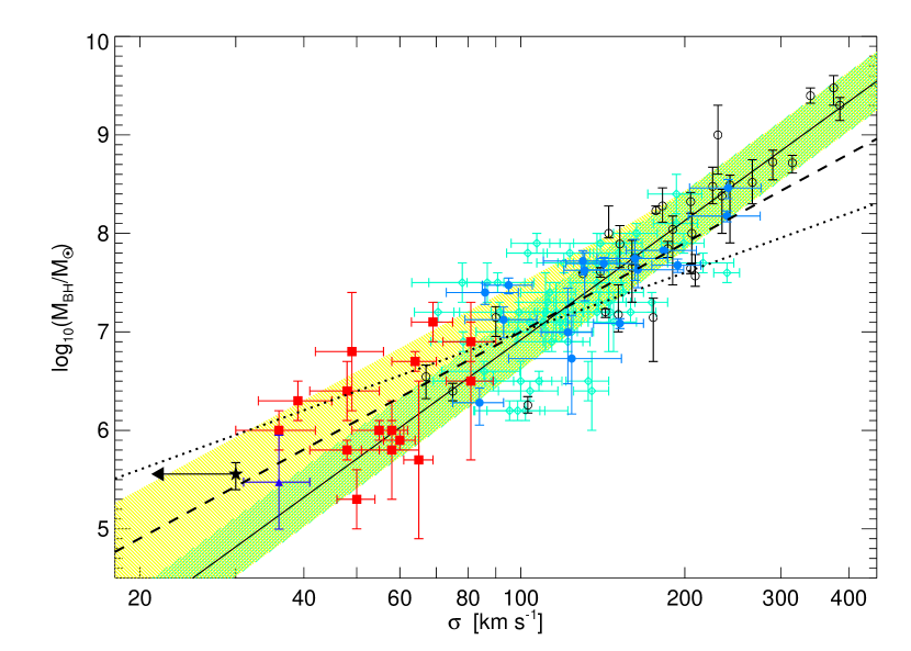
Figure 7.— $M_{\rm BH}-\sigma$ relation measured by Tremaine et al. (2002) (black solid line; $M_{\rm BH}\propto\sigma^{4}$), with estimated intrinsic $0.27$ dex scatter (green shaded range), and the predicted relation at low-$\sigma$ from our model for Seyfert triggering as calculated in § 5.1, given an energy-based feedback coupling (dashed line; $M_{\rm BH}\propto\sigma^{3}$) or momentum-based coupling (dotted line; $M_{\rm BH}\propto\sigma^{2}$). Note that these relations apply only at low $\sigma$ where they lie above the solid line. Yellow range shows the additional scatter expected (for the energy-based coupling, but similar for the momentum-based coupling) calculated from the size spectrum of molecular clouds in § 5.2. For comparison, observations are shown from the compilations of Tremaine et al. (2002) (black open circles), Onken et al. (2004); Nelson et al. (2004); Peterson et al. (2004) (blue filled circles), Barth et al. (2005) (red squares), Greene & Ho (2005a) (cyan diamonds), and of POX 52 from Barth et al. (2004) (purple triangle) and of NGC4395 from Peterson et al. (2005) (black star), for which only an upper limit to $\sigma$ exists (Filippenko & Ho, 2003). The observations tentatively favor the shallower predicted slope and larger scatter at low-$M_{\rm BH}$ from our model, but this remains to be tested with larger samples and more accurate mass determinations.

In Figure 7, we show (solid line) the predicted relation for both merger-driven co-formation of bulges and black holes with $M_{\rm BH}\propto\sigma^{4}$ (Di Matteo et al., 2005), matching the observed relation (Ferrarese & Merritt, 2000; Granato et al., 2000; Tremaine et al., 2002), and for our Seyfert molecular-cloud mode of accretion as predicted by Equation (93) for energy-driven coupling (dashed line) and Equation (95) for a momentum coupling (dotted line). For comparison, observations are shown from various compilations as indicated in the figure caption. Note that the (highly uncertain) reverberation region geometric normalization factor adopted in Greene & Ho (2005a) differs slightly (by $\sim 0.2$ dex) from that of Onken et al. (2004); Nelson et al. (2004); Peterson et al. (2004); Barth et al. (2005). Since we cannot predict the normalization of the $M_{\rm BH}-\sigma$ relation to this accuracy and are, in any case, interested only in the slope and scatter of the relation, we adopt the same normalization for all the samples used.

The comparison between the predicted energy-based relation and the low-mass observations is suggestive. We consider the 37 observed systems below $\sigma\approx 100\,{\rm km\,s^{-1}}$, primarily from the Barth et al. (2005) and Greene & Ho (2005a) samples but also including Pox 52, NGC4395 (for which we adopt the upper limit $\sigma=30\,{\rm km\,s^{-1}}$, as a lower value will only further favor our estimated $M_{\rm BH}-\sigma$ relation over the extrapolated $M_{\rm BH}\propto\sigma^{4}$ relation), and four Tremaine et al. (2002) objects and four Onken et al. (2004) objects. For these objects, if we ignore intrinsic scatter in the relationship, the reduced $\chi^{2}$ of the Tremaine et al. (2002) fitted relation is $\chi^{2}/\nu=16.8$, whereas our prediction gives $\chi^{2}/\nu=12.1$ (an absolute $\Delta\chi^{2}\approx 174$). These are both unacceptable fits, however, so allowing for a constant intrinsic scatter of $0.27$ dex gives $\chi^{2}/\nu=1.72$ (marginally acceptable) for the Tremaine et al. (2002) fit, compared to $\chi^{2}/\nu=1.02$ for our prediction (absolute $\Delta\chi^{2}\approx 26$, still highly significant). Further allowing for the increased intrinsic scatter at low $\sigma$ we predict in § 5.2 below, this drops to $\chi^{2}/\nu=0.21$. Above this $\sigma$, the comparison is not meaningful because we do not predict any substantial correction to the $M_{\rm BH}-\sigma$ relation.

The observations at low black hole masses appear to favor our prediction over a pure bulge and black hole co-formation (i.e. merger-driven) $M_{\rm BH}-\sigma$ relation, which yields a scaling $M_{\rm BH}\propto\sigma^{4}$, roughly independent of mass (see e.g., Di Matteo et al., 2005; Robertson et al., 2005). However, there is only a marginal ($\sim 1-2\sigma$) detection of this trend, and both the measurement errors and systematic uncertainties (e.g., Peterson et al., 2005; Barth et al., 2005; Greene & Ho, 2005b) are large at low masses. Future observations of the $M_{\rm BH}-\sigma$ relation at low masses will provide a strong test of our model, even potentially distinguishing momentum coupling vs. energy coupling models.

5.2. Scatter in the $M_{\rm BH}-\sigma$ Relation

If molecular cloud accretion is important for the growth of low-mass black holes, this mode can influence the scatter in the observed $M_{\rm BH}-\sigma$ relation. For example, the critical $M_{\rm BH}$ for entering the “blowout” phase in Equation (95) is proportional to $R_{\rm cl}^{2}\propto M_{\rm cl}^{2/3}$, so a spectrum of sizes of molecular clouds will introduce scatter in the $M_{\rm BH}-\sigma$ relation. This scatter will be significant if it is larger than the $\sim 0.3\,$dex scatter intrinsic to the $M_{\rm BH}-\sigma$ relation from spheroid-black hole co-formation. The observed scatter in the relationship is approximately constant at high masses (e.g., Tremaine et al., 2002; Novak et al., 2005), and simulations of merger-induced spheroid formation also predict the scatter to remain roughly constant at low masses (Di Matteo et al., 2005; Robertson et al., 2005).

As discussed by McKee & Ostriker (1977), observations of column density distributions in the galaxy (e.g., Hobbs, 1974; Payne et al., 1983; Welty et al., 1994), LMC (e.g., Oestreicher & Schmidt-Kaler, 1996) and AGN hosts (e.g., Tytler, 1987; Hopkins et al., 2004) indicate that the number of clouds per unit column density varies as approximately $N_{H}^{-2}$, implying (for a constant cloud density) that the number of clouds with radii in the range $R\rightarrow R+dR$ per unit volume is $\propto R^{-4}\,dR$. The rate at which clouds collide with the black hole is

$$\frac{dn_{\rm event}}{dt}\sim n_{\rm cl}\,\pi\,R_{\rm cl}^{2}\,v_{\rm cl}\propto\frac{1}{R}\,d\ln{R}\propto\frac{1}{M_{\rm cl}^{1/3}}\,d\ln{M_{\rm cl}},$$ (97)

where $n_{\rm cl}\propto R^{-4}\,dR$ and the independence of $v_{\rm cl}$ and $R$ are used in the second equality. Therefore, the $+1\sigma$ ($68\%$ $R<R^{\prime}$) collision probability corresponds to a cloud about four times larger in radius than our “typical” cloud, i.e. $M_{\rm cl}\sim 70$ times bigger than normal, or $M_{\rm cl}^{2/3}\sim 17.1$ times normal. The $+1\sigma$ dispersion in the $M_{\rm BH}-\sigma$ relation should then be $\approx 1.2$ dex at the lowest $M_{\rm BH}$, larger than the $\sim 0.3$ dex intrinsic to the $M_{\rm BH}-\sigma$ relation determined by co-formation of bulge and black hole.

The lower-$M_{\rm BH}$ limit to the molecular cloud accretion $M_{\rm BH}-\sigma$ relation will be determined by extrapolating the $M_{\rm BH}-\sigma$ relation for co-formation of spheroids and bulges. Although technically the PDF for encountering a cloud of size $R$ (Equation [97]) can be estimated down to the minimum cloud size $\sim 0.5\,$pc, this is unimportant for the scatter in the $M_{\rm BH}-\sigma$ relation. For $R\ll 10-100\,$pc (i.e. less than “typical” large cloud sizes), the minimum black hole mass to “blowout” from Equation (95) is small, e.g. $M_{\rm BH}\sim 10^{4}\,M_{\sun}$ for $R\ll 10\,$pc (and recall that we are considering intervals in $\log{R}$). Thus the contribution to the $M_{\rm BH}-\sigma$ relation from these small clouds (with masses $\lesssim 10^{4}\,M_{\sun}$ for $R\lesssim 10\,$pc) would be larger than the $M_{\rm BH}$ expected from the co-formation of spheroid and bulge only for very small systems $\sigma\lesssim 25\,{\rm km\,s^{-1}}$, below the range of interest (although these terms do contribute a Coulomb logarithm term to the rate of black hole activation, see § 4.1). However, since the typical timescale for an encounter with a sufficiently large cloud is $t_{\rm event}\sim 10^{10}\,$yr, up to $\exp(-t_{H}/t_{\rm event})\sim 21\%$ of systems may not have had an encounter with a molecular cloud of substantial size at any point, and will have an $M_{\rm BH}$ consistent with the $M_{\rm BH}-\sigma$ relation for black hole-spheroid formation ($M_{\rm BH}\propto\sigma^{4}$), making this the approximate $-1\sigma$ lower limit in the $M_{\rm BH}-\sigma$ relation.

In Figure 7 we show, in addition to the predicted $M_{\rm BH}-\sigma$ relation from molecular cloud accretion, the predicted scatter at each mass (combined yellow and green shaded areas). We assume a constant $0.27\,$dex scatter for the spheroid-black hole co-formation $M_{\rm BH}-\sigma$ mechanism with $M_{\rm BH}\propto\sigma^{4}$ (Tremaine et al., 2002), shown as the shaded green range. We could equivalently show the scatter as a function of mass from simulations of merger-driven spheroid formation (Robertson et al., 2005), which span a wide range in final bulge/spheroid masses and have approximately constant $\sim 0.3$ dex scatter.

The observations indicate that the scatter increases at small black hole mass. Greene & Ho (2005a) estimate a scatter of $\sim 0.4$ dex primarily in the range $\sigma\sim 100-200\,{\rm km\,s^{-1}}$, and this appears to increase marginally to $\sim 0.6-0.8$ dex if we consider the objects below $\sigma\sim 75\,{\rm km\,s^{-1}}$. The increased scatter our model predicts at low black hole masses is evident. Quantitatively, however, this change in scatter in the observations is only marginally ($\sim 1\sigma$) significant if we consider points at $\sigma<200\,{\rm km\,s^{-1}}$, where the predicted (yellow) scatter begins to increase over the constant (green) scatter, owing to both the relatively small number of points at the lowest masses and the relatively large measurement errors.

5.3. Accretion of Molecular Clouds at Low $M_{\rm BH}$

The condition for blowout, assuming the black hole energy or momentum couples to the surrounding medium, implies a shallower $M_{\rm BH}-\sigma$ relation, with increased scatter, at low black hole masses. However, a precondition for this is that the black hole be able to efficiently accrete a molecular cloud. If the cloud is moving at a velocity $c_{s}^{\rm disk}$, then the crossing timescale during which the cloud interacts with the black hole is

$$t_{\rm cross}=\frac{R}{c_{s}^{\rm disk}}=1.0\times 10^{7}\,{\rm yr}\,{\Bigl{(}}\frac{R}{100\,{\rm pc}}{\Bigr{)}}\,{\Bigl{(}}\frac{c_{s}^{\rm disk}}{10\,{\rm km\,s^{-1}}}{\Bigr{)}}^{-1}\,,$$ (98)

significantly shorter than the Salpeter time, $t_{S}=4.2\times 10^{7}\,$yr, so the black hole cannot grow by more than a factor of $\sim 3$ in mass in this time interval. Any remaining accretion must come from mass captured in the passage of the cloud.

For a cloud moving at a bulk velocity $c_{s}^{\rm disk}$, the portion of the cloud which passes within a radius

$$R \lesssim \frac{2\,G\,M_{\rm BH}}{(c_{s}^{\rm disk})^{2}}$$ (99)

$$\approx 89\,{\rm pc}\,{\Bigl{(}}\frac{M_{\rm BH}}{10^{6}\,M_{\sun}}{\Bigr{)}}$$

can be “captured” (i.e. bound to the black hole). On average, a fraction $\sim(R/R_{\rm cl})^{2}$ (given by the cross section of a cloud passing over a black hole which does not successfully capture it) of the cloud volume/mass is then available for accretion. For large black holes, this is more than sufficient to power the blowout, and indeed much will not be accreted once the blowout begins. For small enough black holes, however, relatively little mass can be captured. The captured mass is

$$\frac{M_{\rm capt}}{M_{\rm BH}}\sim 10\,{\Bigl{(}}\frac{M_{\rm BH}}{10^{6}\,M_{\sun}}{\Bigr{)}}\,{\Bigl{(}}\frac{R_{\rm cl}}{100\,{\rm pc}}{\Bigr{)}}$$ (100)

(with a maximum at $M_{\rm capt}=M_{\rm cl}$) and so a low-mass black hole can grow only by at most about one order of magnitude from an individual interaction with a typical cloud. If the black hole grows rapidly from the beginning of the interaction, this will still only increase this by a further factor $\sim 2-3$, based on the comparison of the crossing time to the Salpeter time above. For the black hole masses plotted in Figure 7, this is sufficient to account for the movement of black holes from the spheroid-black hole co-formation $M_{\rm BH}-\sigma$ relation ($M_{\rm BH}\propto\sigma^{4}$) to the molecular cloud-dominated $M_{\rm BH}-\sigma$ relation ($M_{\rm BH}\propto\sigma^{3}$), and to provide the mass to power the “blowout”. Of course, a significant ($+1\sigma$) fraction of black holes can interact with larger clouds or torii/disk inflows of sizes up to $\sim 400\,$pc (as calculated in § 5.2 above), allowing a factor $\sim 200$ growth in the black hole mass.

However, for low initial black hole masses $\sim 10^{2}-10^{3}\,M_{\sun}$, as for seed black holes from Population III stars, this is only marginally sufficient to grow black holes to substantial masses (to subsequently act as seeds for further Seyfert accretion or growth in mergers). These seeds likely formed at high redshifts $z\sim 10-20$, when gas densities were large and gas fractions were of order unity, implying a higher effective “collision rate” with dense gas. The Eddington ratio in these phases for undermassive black holes is $\dot{m}\approx 1$, so the timescale for this growth from the captured mass is $\approx 1-2\times 10^{8}$ yr, short enough compared to the age of the Universe for the buildup of seeds which could then grow larger in later mergers.

5.4. Mass Gain in the Blowout Phase

Black holes can also grow during the “blowout” phase. For a power-law decay of the accretion rate with $\dot{m}=(t/t_{\dot{m}})^{-\eta_{L}}$ (Equation [52]), the mass gained can be estimated simply if it is small and we can approximate $\dot{M}=\dot{m}\,\dot{M}_{\rm Edd}=\dot{m}\,M_{\rm BH}/t_{S}$, where $M_{\rm BH}$ is the initial black hole mass. This yields

$$\frac{\Delta M_{\rm BH}}{M_{\rm BH}} = \int\frac{\dot{M}}{M_{\rm BH}}{\rm d}t=\int\frac{{\rm d}t}{{\rm d}\log{\dot{m}}}\,\frac{\dot{m}}{t_{S}}\,{\rm d}\log{\dot{m}}$$ (101)

$$= \eta_{L}\,\frac{t_{\dot{m}}}{t_{S}}\int^{1}_{\dot{m}_{\rm min}}\dot{m}^{-1/\eta_{L}}\,{\rm d}\dot{m}$$

$$= \frac{t_{\dot{m}}}{t_{S}}\ \frac{\eta_{L}}{1-1/\eta_{L}}[1-\dot{m}_{\rm min}^{1-1/\eta_{L}}].$$

Because $\dot{m}_{\rm min}\ll 1$, if $\eta_{L}\geq 1$ then the above becomes

$$\frac{\Delta{M_{\rm BH}}}{M_{\rm BH}} \approx \frac{t_{\dot{m}}}{t_{S}}\ \frac{\eta_{L}}{1-1/\eta_{L}}\ \ \ \ \eta_{L}>1$$ (102)

$$= \frac{t_{\dot{m}}}{t_{S}}\ \ln(\dot{m}_{\rm min}^{-1})\ \ \ \ \eta_{L}=1$$

$\sim t_{\dot{m}}/t_{S}\ll 1$, and indeed the mass gained in the blowout is small. Similarly, $\eta_{L}=1$ contributes an additional logarithmic term $\ln(1/\dot{m}_{\rm min})$, which still leaves $\Delta{M_{\rm BH}}/M_{\rm BH}\ll 1$.

For $\eta_{L}<1$, this becomes slightly more complicated, but ultimately gives a similar result. Because $\dot{m}_{\rm min}\ll 1$, this implies $\Delta{M_{\rm BH}}/M_{\rm BH}\propto\dot{m}_{\rm min}^{1-1/\eta_{L}}$. Using the determination of $\dot{m}_{\rm min}$ from Equation (88), this simplifies to

$$\frac{\Delta{M_{\rm BH}}}{M_{\rm BH}}=f{(\eta_{L})}\,{\Bigl{(}}\frac{\sigma}{100\,{\rm km\,s^{-1}}}{\Bigr{)}}\,,$$ (103)

where $f{(\eta_{L})}$ is a function of $\eta_{L}$ which varies smoothly from e.g. $f(\eta_{L}=1/2)=0.4$ to $f(\eta_{L}\rightarrow 0)\rightarrow 1.8$. Therefore, for sufficiently low values of $\eta_{L}$, the accretion rate decays slowly enough that some mass gain is possible in the blowout.

However, the growth is still relatively small, a factor $\lesssim 2$, and less for lower-mass disks. A full numerical calculation allowing for the increase in mass with low-$\eta_{L}$ changing the Eddington luminosity as the accretion rate decays also gives a small correction of a factor $\lesssim 2$ to the duty cycle at the lowest luminosities. This is consistent with detailed simulations of X-ray driven winds, which suggest efficient wind driving for $L/L_{\rm Edd}>0.08$ (Balsara & Krolik, 1993), implying (given the large observed energetics of AGN outflows) that most of the energy of the system should be generated in this early phase. This is also a potential source of increased scatter in the $M_{\rm BH}-\sigma$ relation, but is at most comparable to the observed scatter (e.g., Tremaine et al., 2002; Novak et al., 2005) and that expected from merger-driven co-formation of spheroids and black holes, and is much smaller than the scatter expected from the accretion of different mass molecular clouds given the blowout conditions as discussed in § 5.2.

6. Obscuration and the Classic Molecular Torus

6.1. Obscuration as a Function of Luminosity

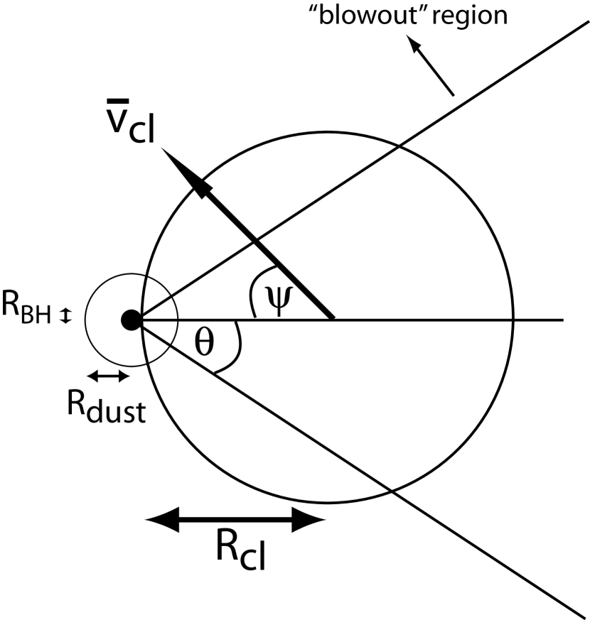
Figure 8.— Illustration of the geometry at first interaction of a cloud and black hole, with cloud radius $R_{\rm cl}$, black hole radius of influence $R_{\rm BH}$, dust sublimation radius $R_{\rm dust}$, and cloud velocity $\bar{v}_{\rm cl}\sim c_{s}^{\rm disk}$.

If a molecular cloud is accreted and not all is subsequently disrupted by feedback, then some fraction of sightlines to the black hole will pass through the surviving portion of the cloud and will be highly obscured. From our momentum coupling considerations of blowout, we can estimate this fraction as a function of luminosity or black hole mass.

Consider a cloud approaching the black hole at the time where the black hole is about $\sim R_{\rm cl}$ from cloud center (i.e. first “touching” the cloud), as illustrated in Figure 8. Since $R_{\rm BH}\ll R_{\rm cl}$ this indeed defines their “initial” interaction. The cloud is moving with a local velocity $c_{s}^{\rm disk}$, at an angle $\psi$ relative to the axis connecting the black hole and cloud center. Define $\theta$ as the angle from this axis to a given point in the cloud, with the black hole at the origin (defining a ray $\bar{r}$), and let $\phi$ be the angle about this axis of symmetry. Thus the cloud velocity relative to the black hole is $\bar{v}=c_{s}^{\rm disk}\,\hat{v}$ with $\hat{v}=\sin{\psi}\,\hat{x}-\cos{\psi}\hat{z}$. The linear momentum of a given parcel of gas along such a ray originating at the black hole, against the direction of the ray, is then

$${\rm d}{|{p}|} = {\rm d}M\,c_{s}^{\rm disk}\,(-\hat{r}\cdot\hat{v})$$ (104)

$$= \rho_{\rm cl}\,c_{s}^{\rm disk}\,r^{2}\,\sin{\theta}\,(-\sin{\theta}\,\cos{\phi}\,\sin{\psi}+\cos{\theta}\,\cos{\psi})\,{\rm d}r\,{\rm d}\theta\,{\rm d}\phi$$

$$= \frac{8\pi}{3}\,\rho_{\rm cl}\,R_{\rm cl}^{3}\,c_{s}^{\rm disk}\,\cos{\psi}\,\sin{\theta}\cos^{4}{\theta}\,{\rm d}\theta$$

$$= 2\,M_{\rm cl}\,c_{s}^{\rm disk}\,\cos{\psi}\,\cos^{4}{\theta}\,{\rm d}{\cos{\theta}}\,,$$

where the third equality comes from integrating over $\phi$ and $r$ (from $r\sim R_{\rm BH}\ll R_{\rm cl}$ to $r=2\,R_{\rm cl}\,\cos{\theta}$).

Consider the portion of the cloud with $\theta>\theta_{0}$, then the total momentum input to “clear” a sightline in this fraction of the cloud is

$$|p|=\frac{2}{5}\,\cos{\psi}\,M_{\rm cl}\,c_{s}^{\rm disk}\,\cos^{5}\theta_{0}\,.$$ (105)

Since by our definitions $0\leq\psi\leq\pi/2$, $\langle\cos{\psi}\rangle=2/\pi$, so

$$\langle p\rangle=\frac{4\pi}{5}M_{\rm cl}\,c_{s}^{\rm disk}\,\cos^{5}\theta_{0}\,.$$ (106)

If the radiation from the black hole is directed isotropically and impacts the cloud, at least initially, via momentum coupling, the momentum imparted in some time interval $\Delta t$ is then ${\rm d}p=\eta\,(L\,\Delta t/c)\,({\rm d}\Omega/4\pi)$, where ${\rm d}\Omega$ is the opening angle considered and $\eta$ is the coupling efficiency. Considering the range above, with $\theta_{0}\leq\theta\leq\pi/2$, this gives $\Delta\Omega=\int{\rm d}\Omega=2\pi\,\cos{\theta_{0}}$, so the total momentum input from the black hole in this region is

$$p_{\rm BH}=\frac{1}{2}\,\eta\,\frac{L\,\Delta t}{c}\,\cos{\theta_{0}}\,.$$ (107)

This will be sufficient to overwhelm the momentum of the cloud and blow out material with $\theta>\theta_{0}$ for

$$\cos{\theta_{0}} > \ {\Bigl{[}}\frac{5}{8\pi}\eta\,\frac{L\,\Delta t}{M_{\rm cl}\,c_{s}^{\rm disk}\,c}{\Bigr{]}}^{1/4}$$

$$= {\Bigl{[}}\frac{1}{4\pi}\eta\,\epsilon_{r}\,\dot{m}\,\frac{M_{\rm BH}}{M_{\rm cl}}\,\frac{R_{\rm cl}\,c\,\tau_{\ast}}{t_{S}\,c_{s}^{\rm disk}\,\sigma}{\Bigr{]}}^{1/4}$$

$$= 0.8\,(\eta\,\tau_{\ast}\,\dot{m})^{1/4}\,{\Bigl{(}}\frac{R_{\rm cl}}{100\,{\rm pc}}{\Bigr{)}}^{-1/2}\,{\Bigl{(}}\frac{M_{\rm BH}}{10^{7}\,M_{\sun}}{\Bigr{)}}^{3/16}$$

$$\approx 0.6\,(\eta\,\tau_{\ast})^{1/4}\,{\Bigl{(}}\frac{R_{\rm cl}}{100\,{\rm pc}}{\Bigr{)}}^{-1/2}\,{\Bigl{(}}\frac{L}{10^{11}\,L_{\sun}}{\Bigr{)}}^{1/4}\,,$$

where we have used $\Delta t=t_{\dot{m}}\sim R_{\rm cl}/\sigma$, the characteristic timescale for the blast wave impact.

Thus, for sufficiently low luminosities or black hole masses, there is some solid angle in which feedback cannot “punch through” the cloud, and the cloud will remain as an obscurer. The covering angle for this is

$$f=\frac{1}{2}(1-\cos{\theta_{0}})\,.$$ (109)

This is similar to our derivation of the blowout criterion as a function of mass in § 5.1, and here we incorporate the geometric effects of “partial” blowout. These partially obscured objects will be visible as Seyfert 2’s, with properties consistent with the canonical molecular torus unification model.

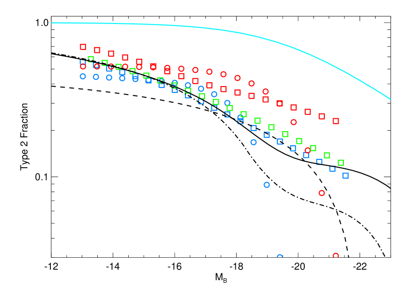
Figure 9.— Predicted Seyfert 2 fraction as a function of luminosity, calculated from our modeling of a pressure-driven blast wave (black lines). Dashed line uses the simplified luminosity criterion of Equation (6.1), dot-dashed line includes the more detailed dependence on $M_{\rm BH}$ (integrating over the high-accretion rate period), solid line further includes integration over a spectrum of cloud sizes. Points show the observed Type 2 fraction from the local AGN luminosity functions of Hao et al. (2005), using Schechter (circles) and double power-law (squares) function fits to H$\alpha$ (blue), [OII] (red), and [OIII] (green) observations, converted as in Figure 2. For comparison, the fitted Type 2 fraction from Simpson (2005), determined from the samples therein and from Ueda et al. (2003); Hasinger (2004); Grimes, Rawlings, & Willott (2004), and dominated by quasars with $0\lesssim z\lesssim 3$ (i.e. merger-driven quasar activity and obscuration in our modeling; see Figure 6 and Hopkins et al. 2006a) is shown (cyan line).

In Figure 9, we show the predicted fraction of Seyfert 2’s as a function of luminosity from the luminosity-dependent form of Equation (6.1). For comparison, we plot the estimated Seyfert 2 fraction from observations as indicated, in the manner of Figure 2. The predicted scaling agrees with the observed trend, and also defines a cutoff at $L\sim 10^{11}-10^{12}\,L_{\sun}$, i.e. $M_{B}\sim-19$ to $-21$, above which the requirement for obscuration is $\cos{\theta_{0}}>1$; i.e. the black hole is sufficiently luminous to destroy the entire cloud regardless of angle.

There are, however, two detailed effects which will smooth this cutoff. First, the pure luminosity form of Equation (6.1), while giving the appropriate scaling, is not strictly appropriate since the blowout in a given direction may not depend on the instantaneous Seyfert luminosity, which may have decayed to quite low luminosities at later times, but on the momentum injected in the initial, high-luminosity “blowout” phase. This is given by re-considering Equation (6.1), as a function of black hole mass, with $\dot{m}=1$ for a period $t_{\dot{m}}$ as determined in § 3.2 (technically we integrate from $\dot{m}=1$ to $\dot{m}\lesssim 0.1$, since we define a differential time per logarithmic interval in accretion rate). This then provides a more precise estimate of the fraction which will have been “blown out” by the blast wave. Accounting for this yields the dot-dashed line in Figure 9. At a given luminosity, there is a distribution of black hole masses at various accretion rates, and this effect smooths the obscured fraction as a function of luminosity. However, this still defines a characteristic $M_{\rm BH}\sim 10^{8}\,M_{\rm sun}\gg M_{\rm cl}$ above which the blowout will completely disrupt the cloud, with a corresponding Eddington luminosity $L\sim 10^{12}\,L_{\sun}$.

The second effect is the spectrum of cloud sizes. A more or less massive cloud also implies a correspondingly smaller or larger covering angle of material which cannot be expelled. We use the spectrum of cloud sizes in § 5.2 to calculate the dispersion in the $M_{\rm BH}-\sigma$ relation expected from this mode of accretion, and an identical calculation gives the dispersion in $M_{\rm cl}$ and correspondingly, via Equation (6.1), the variation in obscured fractions as a function of $M_{\rm BH}$. Averaging over this distribution yields the total obscured fraction as a function of $M_{\rm BH}$ and $L$, shown as the solid black line in Figure 9.

These more detailed effects produce significant differences at intermediate masses, where the transition between obscured and unobscured populations is smoothed out. The agreement with the observations is improved, suggesting that this momentum balance argument provides a plausible estimate of the obscured fraction as a function of luminosity.

Note also that our argument does not necessarily depend on the black hole luminosity affecting directly the surrounding medium via radiation pressure or other momentum couplings. Rather, because the blast wave impacting the medium will be pressure-driven, $\eta$ as used above represents an effective efficiency of the Seyfert energy and momentum “ending up” in the initially driven blast wave by the time it impacts on the surrounding medium.

Our prediction is qualitatively similar to those of various modified “luminosity-dependent” torus models, and the fundamental qualitative point, that black hole feedback which is stronger in higher-luminosity systems is able to clear a larger opening angle, still obtains. However, our result is distinct from some of these models in several respects. For example, the “receding torus” model (e.g., Lawrence, 1991) assumes that the opening angle increases as the inner torus radius increases, owing to a larger dust sublimation radius $r_{\rm dust}\propto L^{1/2}$ with increasing dissociating luminosity. However, while this gives a reasonable scaling of the obscured fraction for a geometrically flat (i.e. rectangular torus cross-section) torus, it is clear from Figure 8 that for an increasing torus radius with $r$ (i.e. a circular torus cross-section or elliptical/spherical cloud, and conical opening angle models), removing a spherical region around the origin at the black hole has almost no effect on the covering angle of the cloud. This is true until $r_{\rm dust}\gg R_{\rm cl}$ (for example, even at $r_{\rm dust}=R_{\rm cl}$, for a spherical cloud or circular torus cross section, this only decreases the Type 2 fraction by a factor of two from $r_{\rm dust}=0$). In other words, the dust sublimation radius would have to reach $\sim 10-100\,$pc before this mechanism would explain a scaling of obscured fraction with luminosity in this fueling scenario, into (or even beyond) the traditional narrow line regions.

Qualitatively, our mechanism is more similar to the disk-wind model of Konigl & Kartje (1994); Elvis (2000); Proga & Kallman (2004), in which radiation pressure flattens the initially vertical outflow and dust distribution in objects with higher bolometric luminosities. However, it can operate on much larger scales and depends on momentum balance from the blast wave (not necessarily direct radiation pressure) ejecting material within some opening angle, rather than merely flattening the distribution. It is also worth noting the striking similarity of the obscured fraction calculated from Equations (6.1) and (109) and the functional form of empirical calculations which allow for e.g. evolution of the inner torus radius and torus height as a function of luminosity (e.g., Simpson, 2005), suggesting that feedback balance does capture the critical dependence on black hole and fueling properties.

For comparison, the fitted Type 2 fraction as a function of luminosity in higher-redshift quasars from Simpson (2005), determined from the SDSS and from Ueda et al. (2003); Hasinger (2004); Grimes, Rawlings, & Willott (2004), is shown as the cyan line in Figure 9. While a similar qualitative trend is apparent, the Type 2 fraction is much higher, completely dominating at low-luminosities and contributing a substantial $\sim 30\%$ portion of the population even at $M_{B}\lesssim-23$, whereas in the local samples the Type 2 fraction is at most comparable to the Type 1 fraction at low luminosities and negligible ($\ll 10\%$) at high luminosities.

The cause of this difference is suggested by Figure 6, in which the Seyfert (i.e. quiescent, cold gas driven) and quasar (i.e. merger-driven) luminosity functions are each plotted at several redshifts. Even by $z\sim 0.1-0.2$, the quasar population is larger at these luminosities, and indeed the Simpson (2005) sample is drawn from surveys which are dominated by quasars at high redshifts spanning the wide range $0.15\lesssim z\lesssim 3$. These objects, in our modeling, are triggered by different processes, and therefore should not necessarily follow the same trend – indeed, the discrepancy between the two observations cautions against extrapolation of obscuration models (e.g. geometrical models) calibrated for local, non-interacting populations. In Hopkins et al. (2005a, b, 2006a) we discuss this obscuration in a merger-driven context in detail, and show that the trends of Ueda et al. (2003); Hasinger (2004); Grimes, Rawlings, & Willott (2004); Simpson (2005) can be reproduced when the primary source of obscuration is produced by larger scale ($\gtrsim 50$ pc) gas inflows from the mergers which themselves power accretion, and the distribution of column densities derives primarily from time-dependent rather than line-of-sight dependent differences. A similar qualitative trend is found because bright systems are more likely to be near their peak luminosity, when they are able to expel obscuring gas and dust, which is similar in principle to the model we have described here for obscuration of cloud-fueled AGN. However, in our model for non-interacting Seyferts, the obscuration is removed along certain sightlines at the beginning, not at the end of black hole growth, and the distribution of $N_{H}$ does, presumably, derive from geometric effects, as in canonical torus or disk-wind models.

6.2. Building a Torus

Although it is not a requirement of this model, our picture for AGN fueling can both derive from and seed the traditional molecular torus of standard AGN unification models. Assuming that a significant fraction of an accreted cloud is captured on passage near the black hole, essentially requiring $R_{\rm cl}\lesssim G\,M_{\rm BH}\,(c_{s}^{\rm disk})^{-2}$, or $M_{\rm BH}\gtrsim 10^{5}\,M_{\sun}$ (ensured for the black hole masses of interest and for the predicted $M_{\rm BH}-\sigma$ relation for this fueling mechanism, see § 5), then it will presumably develop an orbit, circularize, and some fraction of the cloud will be tidally disrupted.

Given an initial impact parameter $b$ and velocity $c_{s}^{\rm disk}$, the material can settle into a Keplerian orbit determined by conservation of angular momentum. For the bulk of the cloud, $b\sim R_{\rm cl}\gg R_{\rm BH}$, so the circular velocity is determined by the spheroid potential,

$$v_{c}=\sigma\,\sqrt{\frac{r}{a}}$$ (110)

where $a$ is the bulge scale-length. Using $a=10\,{\rm kpc}\,(\sigma/{\rm 200\,km\,s^{-1}})^{2}$ from § 3.1 with the appropriate factor of $\tilde{\phi}$ to convert from observed $\sigma$ to a physical $v_{c}$ and $a$ assuming a Hernquist (1990) spheroid profile yields $v_{c}\approx 200\,{\rm km\,s^{-1}}\,\sqrt{r/{\rm kpc}}$. Since this will include most of the mass, demanding the final angular momentum $\sim M\,r\,v_{c}$ (in detail $=(3\tilde{h}^{2}/4+1)\,M\,r\,v_{c}$ for a torus with $\tilde{h}=h/r$) conserve the initial $\sim M\,R_{\rm cl}\,c_{s}^{\rm disk}$ (again, in detail $M\,R_{\rm cl}\,c_{s}^{\rm disk}\,\sin{\psi}$ for the geometry in § 6.1) yields a torus radius

$$R_{\rm t} = R_{\rm cl}\,{\Bigl{(}}\frac{a}{R_{\rm cl}}{\Bigr{)}}^{1/3}\,{\Bigl{(}}\frac{c_{s}^{\rm disk}}{\sigma}{\Bigr{)}}^{2/3}\,{\Bigl{(}}\frac{\langle\sin{\psi}\rangle}{\frac{3}{4}\tilde{h}^{2}+1}{\Bigr{)}}^{2/3}$$ (111)

$$\approx 20\,{\rm pc}\,{\Bigl{(}}\frac{R_{\rm cl}}{100\,{\rm pc}}{\Bigr{)}}^{2/3}\,{\Bigl{(}}\frac{c_{s}^{\rm disk}}{10\,{\rm km\,s^{-1}}}{\Bigr{)}}\,,$$

independent of $\sigma$, and assuming $\tilde{h}\sim 1$ as we show below. Thus the characteristic torus size $\lesssim 10$’s of pc (up to a maximum $\sim 100\,$pc) inferred from a wide variety of observations (Krolik & Begelman, 1988; Granato et al., 1997; Bock et al., 2000; Schinnerer et al., 2000; Galliano et al., 2003; Radomski et al., 2003; Weigelt et al., 2004; Jaffe et al., 2004; Prieto et al., 2004; Elitzur, 2005) and simulations of torus structure and stability with radiative transfer models (e.g., Pier & Krolik, 1993; Granato & Danese, 1994) is a natural consequence of the scales of molecular clouds, and is “built into” this picture of Seyfert fueling.

Given this radius, whether the molecular cloud is circularized into a strict torus with volume $2\pi^{2}\,R_{\rm t}^{3}$ (assuming $\tilde{h}\sim 1$) or remains spherical/ellipsoidal, the change in e.g. density and other gas properties is well-defined (varying by e.g. $20\%$ using the exact solutions above and assuming it goes from a sphere to a torus). Therefore, the characteristic density is also given by that of the original cloud, enhanced by the compression expected from Equation (111) above, explaining the molecular and dust densities and masses inferred for molecular torii around Seyferts, with $n\sim 10^{2}-10^{4}\,{\rm cm}^{-3}$. This gives a line-of-sight column density through the torus plane of

$$N_{\rm H{\small I}}=2\,R_{\rm t}\,n_{\rm t}\approx 2\,R_{\rm cl}\,n_{\rm cl}\,{\Bigl{(}}\frac{R_{\rm cl}}{R_{\rm t}}{\Bigr{)}}^{2}\approx 1.6\times 10^{24}\,{\rm cm^{-2}}.$$ (112)

This is similar to the column densities of torii inferred from phenomenological fits to the complete hard X-ray column density distributions of Seyferts (Urry & Padovani, 1995; Treister et al., 2004; Mainieri et al., 2005) and from synthesis models fitted to the X-ray background (Setti & Woltjer, 1989; Madau et al., 1994; Comastri et al., 1995; Gilli et al., 1999, 2001; Treister & Urry, 2005).

We can also calculate the expected height or flattening of this torus, as a function of radius and Seyfert properties. If the molecular cloud, with density $n_{\rm cl}\sim 100\,{\rm cm^{-3}}$ collapses from the ISM with mean density $n_{\rm ISM}\sim 1\,{\rm cm^{-3}}$, and magnetic flux ($\equiv B\,{\rm d}A\sim B\,R^{2}$) is conserved, the magnetic field will be enhanced by $B_{\rm cl}/B_{\rm ISM}\sim(n_{\rm cl}/n_{\rm ISM})^{2/3}$. For typical magnetic fields providing pressure support in molecular clouds

$$\frac{\partial P}{\partial r}\sim\frac{1}{R_{\rm cl}}\,\frac{B_{\rm cl}^{2}}{4\pi}=\rho\,\frac{\partial\phi}{\partial r}\sim\rho\,\frac{G\,M_{\rm cl}}{R_{\rm cl}^{2}}\,,$$ (113)

with $B_{\rm cl}=B_{\rm ISM}\,(n_{\rm cl}/n_{\rm ISM})^{2/3}$ and $M_{\rm cl}=(4\pi/3)\,R_{\rm cl}^{3}\,\rho$. For a diffuse ISM $B_{\rm ISM}\sim$ a few $\mu G$, this yields

$$R_{\rm cl}\sim 100\,{\rm pc}\,{\Bigl{(}}\frac{B_{\rm ISM}}{4\,\mu G}{\Bigr{)}}\,,$$ (114)

giving the standard self-consistent picture for the magnetic support (in addition to support from turbulent motions) for molecular clouds, with these field strengths characteristic of the disordered fields of the Milky Way ISM (e.g. Troland & Heiles 1986; Rand & Kulkarni 1989; for a review see e.g. Ferriere 2001). Increasing magnetic field strengths are also observed towards the center of the Galaxy, up to a factor of $\sim 10$ larger, supporting higher densities and even larger giant molecular cloud complexes with $M_{\rm cl}$ up to $\sim 10^{8}\,M_{\sun}$ (e.g., Rand & Lyne, 1994; Myers et al., 1995; Myers & Khersonsky, 1995; Crutcher, 1999).

Because capture and circularization does not completely erase the properties of the molecular cloud, the magnetic fields on cloud scales can be preserved, continuing to provide pressure support. This pressure defines an effective sound speed $c_{B}^{2}=(B_{\rm cl}^{2}/4\pi)\,\rho^{-1}$, which for the above is $c_{B}\approx 20\,{\rm km\,s^{-1}}\,(B_{\rm ISM}/4\,\mu G)$. Note that any other source of a similar pressure which is non-thermal (i.e. does not scale adiabatically), such as e.g. turbulent motions, will have a similar effect. Since this dominates the pressure support of the torus, and using the circular velocity at $R_{\rm t}\gg R_{\rm BH}$ (i.e. dominated by the spheroid potential) the scale height is

$$\tilde{h} \equiv \frac{H_{\rm t}}{R_{\rm t}}\sim{\Bigl{(}}\frac{c_{B}}{v_{c}}{\Bigr{)}}=\sqrt{\frac{a}{R_{\rm t}}}\,{\Bigl{(}}\frac{c_{B}}{\sigma}{\Bigr{)}}$$ (115)

$$\approx 0.70\,{\Bigl{(}}\frac{R_{\rm cl}}{100\,{\rm pc}}{\Bigr{)}}^{-1/3}\,,$$

with a maximum of $H_{\rm t}\sim R_{\rm cl}$. Thus, the torus is not expected to be strongly compressed, at the outer radii, with $H_{\rm t}\sim R_{\rm t}$, again similar to traditional phenomenological models and observational estimates of the torus structure and covering angle (Krolik & Begelman, 1988; Antonucci, 1993; Urry & Padovani, 1995; Risaliti et al., 1999; Schmitt, 2001).

The timescale for all of this to occur will be of order the orbital timescale, $t_{\rm orb}\sim r/v_{c}$, or $\sim R_{\rm cl}/c_{s}^{\rm disk}\sim 10^{7}\,{\rm yr}$ for the bulk of the cloud at $R_{\rm t}\sim R_{\rm cl}$. Thus, if the cloud is captured, it will begin to reach an equilibrium in the blast wave and orbit with the circular velocity in roughly a crossing time. It is therefore expected that it will be seen as such over the majority of the Seyfert lifetime. There is a period of time $\sim 10^{7}\,$yr, comparable to the timescale at highest accretion rates $\dot{m}\gtrsim 0.1$, during which the system may be settling into equilibrium. We have shown the transition from cloud to torus implies little change in the cloud properties, so observational signatures of this transition phase, if it occurs, may not be obvious.

7. Global Consequences for the Host Galaxy

Given the effects of the black hole feedback we have modeled, and the fact that the blast wave can propagate to large ($\sim\,$kpc) scales on reasonable ($\sim\,$Gyr) timescales, in principle there could be a significant impact on the host galaxy ISM or gas structure. The black hole feedback expected from growth in mergers can sweep a large fraction of the remaining gas in the galaxy into an unbound blast wave, heating the remaining gas to the virial temperature and terminating star formation (Hopkins et al., 2006a, c; Springel et al., 2005a). However, the case of fueling by molecular cloud accretion is quite different, and we find that the blast wave is much weaker than required to significantly impact the host galaxy.

If the blowout is defined by the criterion that $M_{\rm cl}$ be accelerated to $v_{\rm esc}\sim\sigma$ (i.e. that the local gas be unbound), then because $M_{\rm cl}\ll M_{\rm ISM}$, a collision between the blast wave and the ISM will at most accelerate the ISM to $\sim(M_{\rm cl}/M_{\rm ISM})\,\sigma$, if momentum considerations are most important. For typical Galactic scales this gives a bulk speed $\ll 1\,{\rm km\,s^{-1}}$, which is completely negligible on the scales of the ISM. Even under the extreme assumption that all the blast wave energy can be converted into bulk motion gives a velocity $\sim\sqrt{M_{\rm cl}/M_{\rm ISM}}\,\sigma\lesssim 1\,{\rm km\,s^{-1}}$. Thus, the blast wave itself is not expected to significantly impact the host galaxy ISM.

If, instead of the momentum or energy in the blast wave shell, we make an even more extreme assumption that all of the feedback energy or momentum flux from black hole growth impacts the galaxy ISM, the energy input could be much larger. We further make the maximal assumptions that $\eta_{L}$ is small, so the black hole grows substantially (by a factor $\sim 2$, see § 5.4), and that the affected ISM is unable to radiate. Let us also consider the case of direct energy coupling (i.e. conversion of all feedback energy into bulk motion), which gives an increased impact of feedback by a factor $\sim c/\sigma\sim 10^{3}$ over e.g. momentum-based coupling. Then, the feedback energy from the black hole is $\sim\eta\,\epsilon_{r}\,M_{\rm BH}\,c^{2}\,\Delta\Omega$, where $\Delta\Omega$ is the covering angle of the disk to the black hole, since the radiation is isotropic. Note that collimation will tend to be perpendicular to the disk and along the angular momentum vector, meaning it will only moderate the impact on the host galaxy.

The binding energy of the disk gas is $\sim f_{\rm gas}\,M_{\rm d}\,v_{c}^{2}$. Using the fact that $M_{\rm BH}\sim\mu M_{\rm b}$, where $M_{\rm b}$ is the bulge mass, this implies that the black hole feedback will be significant (i.e. comparable to the binding energy of the disk ISM gas) when

$$v_{c}^{2}\sim\frac{\epsilon_{r}\,\eta\,\mu}{f_{\rm gas}}\,\frac{M_{\rm b}}{M_{\rm d}}\,\Delta\Omega\,c^{2}\,.$$ (116)

Since the disk covering angle (weighted over the mass/volume of the disk) is $\theta\sim h_{\rm d}/r_{\rm d}\sim c_{s}^{\rm d}/v_{c}$, and the covering factor is $(1-\cos{\theta})\rightarrow\theta^{2}/2$, and we expect $\mu\sim 0.001$, $\eta\sim 0.01$, $c_{s}^{\rm disk}\sim 10\,{\rm km\,s^{-1}}$, we can solve for the maximum $v_{c}$ for which black hole feedback will have a large impact. This gives

$$v_{c}\sim 36\,{\rm km\,s^{-1}}\,{\Bigl{[}} {\Bigl{(}}\frac{\epsilon_{r}}{0.1}{\Bigr{)}}\,{\Bigl{(}}\frac{f_{\rm gas}}{0.1}{\Bigr{)}}^{-1}\,{\Bigl{(}}\frac{\eta}{0.01}{\Bigr{)}}\,$$ (117)

$$\times{\Bigl{(}}\frac{\mu}{0.001}{\Bigr{)}}\,{\Bigl{(}}\frac{{\rm B/T}}{0.1}{\Bigr{)}}{\Bigr{]}}^{1/4}$$

i.e. $M_{\rm d}\lesssim 10^{9}\,M_{\sun}$ with $M_{\rm BH}\lesssim 10^{5}\,M_{\sun}$. Again, this assumes the entire energy output of the black hole has a chance to couple to the ISM with no allowance for that ISM to dynamically relax or cool, and thus represents the most extreme estimate of which galaxies could be affected. Such low-mass galaxies will typically be later types than the Sa/b’s with typical B/T$\sim 0.1$ above, more likely $\lesssim 0.02$ for Sc/d and Sm/Im galaxies, and gas fractions potentially quite a bit higher than $\sim 0.1$, making the host even more robust against black hole feedback. If we consider a momentum coupling ($\sim\eta\epsilon_{r}\,M_{\rm BH}\,c$ compared to $f_{\rm gas}\,M_{\rm d}\,v_{c}$) criteria instead, then we obtain

$$v_{c}\sim 0.2\,{\rm km\,s^{-1}}\,{\Bigl{[}} {\Bigl{(}}\frac{\epsilon_{r}}{0.1}{\Bigr{)}}\,{\Bigl{(}}\frac{f_{\rm gas}}{0.1}{\Bigr{)}}^{-1}\,{\Bigl{(}}\frac{\eta}{1.0}{\Bigr{)}}\,$$ (118)

$$\times{\Bigl{(}}\frac{\mu}{0.001}{\Bigr{)}}\,{\Bigl{(}}\frac{{\rm B/T}}{0.1}{\Bigr{)}}{\Bigr{]}}^{1/3}\,,$$

a negligible effect.

8. The Contribution of Stellar Wind Fueling

For comparison, we briefly consider the contribution of stellar winds and hot (virialized) gas fueling to AGN activity. First, consider the contribution of stellar winds from the galaxy as a whole – these will, in general, shock against one another and virialize, contributing to the hot gas reservoir which can be accreted through the Bondi radius. Assuming the gas is virialized gives $c_{s}^{2}=3\tilde{\phi}\,\sigma^{2}$, where the dimensionless factor $\tilde{\phi}$ depends on the density profile and converts between the observed mean projected velocity dispersion within the effective radius ($\sigma$) and the potential at $z=0$ ($\tilde{\phi}\approx 10.1$ for a Hernquist [1990] spheroid profile). We further use the radial hydrostatic equilibrium condition to solve for $\rho$, which gives a profile having a core with a characteristic $n_{\rm ISM}\sim 1\,{\rm cm^{-3}}$ at the center. Using this and the $M_{\rm BH}-\sigma$ relation, we obtain

$$\dot{m} = 4\pi\alpha\,\frac{G^{2}\,M_{\rm BH}\,t_{S}\,\rho}{\sigma^{3}}\,{\Bigl{(}}\frac{\sigma^{2}}{c_{s}^{2}+v^{2}}{\Bigr{)}}^{3/2}$$ (119)

$$\approx 6.0\times 10^{-5}\,{\Bigl{(}}\frac{n_{\rm ISM}}{1\,{\rm cm^{-3}}}{\Bigr{)}}\,{\Bigl{(}}\frac{\sigma}{200\,{\rm km\,s^{-1}}}{\Bigr{)}}$$

where we have also taken $\gamma=5/3$ (giving $\alpha=1/4$ for the Bondi-Hoyle solution) in the second equality.

Ciotti et al. (1991) consider a detailed numerical calculation of injection of gas into the hot ISM from steady stellar mass loss, supernova events, and galaxy-scale inflows and outflows. For each of their range of conditions, we consider the temperature, gas velocity, and density at the trans-sonic radius for inflow (in the solutions they consider with a central mass concentration) and compare the implied Bondi rate with that estimated above, and arrive at a similar result (to within a factor $\sim 2-3$). This also agrees with the Bondi rates estimated from systematic measurements of hot gas temperature and density profiles in the inner regions of a number of quiescent ellipticals (e.g., Pellegrini, 2005; Soria et al., 2005b). The characteristic $\dot{m}\sim 10^{-5}-10^{-4}$ from galaxy scale hot virialized gas appears to be a robust result. Note that while the total stellar mass loss rate of a quiescent elliptical can be $\sim 1\,M_{\sun}\,{\rm yr^{-1}}$ under typical conditions, the calculations of Ciotti et al. (1991) and others have shown that a far smaller fraction of this gas actually reaches the center of the galaxy, and it does so either at super-$\sigma$ bulk velocities (if un-shocked) or $\sim\sigma$ sound speeds (if shocked and virialized), giving a much lower actual Bondi rate for black hole accretion.

Following Soria et al. (2005a, b), we also estimate the total stellar mass loss within the black hole radius of influence. Winds within this radius will be captured by the black hole, and be available for accretion. Note that, strictly speaking, this is appropriate only for wind velocities $v_{w}<\sqrt{\tilde{\phi}}\sigma$ (the spheroid escape velocity at the center), as otherwise the capture radius is smaller than the radius of influence. For typical slow wind speeds $\sim 100-300\,{\rm km\,s^{-1}}$, however, this is at most comparable to typical ellipticals $\sqrt{\tilde{\phi}}\sigma$, making this a relatively small source of uncertainty. This will, however, restrict the ability of e.g. a young stellar cluster near the nucleus (with much higher $\dot{M}$ in winds than older stellar populations) to contribute significantly to moderate or high-$\dot{m}$ populations, as with typical $v_{w}$ up to $\sim 1000\,{\rm km\,s^{-1}}$, the effective volume in which such systems can have their winds captured is dramatically reduced, and furthermore the large bulk velocity reduces the estimated Bondi rate.

For steady mass loss from older stellar populations, we adopt the estimate of Ciotti et al. (1991) from population synthesis for the mass loss rates as a function of the spheroid age

$$\dot{M}(t)=1.5\times 10^{-11}\,{\Bigl{(}}\frac{L_{B}}{L_{\sun,\,B}}{\Bigr{)}}\,{\Bigl{(}}\frac{t}{15\,{\rm Gyr}}{\Bigr{)}}^{-1.3}\,M_{\sun}\,{\rm yr^{-1}}.$$ (120)

Using a constant mass-to-light ratio $\lambda=(M_{\sun}/L_{\sun,\,B})/(M_{\rm bulge}/L_{B})$, and modeling the spheroid stars with a Hernquist (1990) profile to calculate the mass fraction within $R_{\rm BH}\equiv G\,M_{\rm BH}/\sigma^{2}$, then using the black hole-bulge mass correlation of Marconi & Hunt (2003) to cancel the dependence on $M_{\rm BH}/M_{\rm bulge}$, we obtain

$$\dot{m}\approx 1.1\times 10^{-4}\,\lambda\,{\Bigl{(}}\frac{M_{\rm BH}/M_{\rm bulge}}{0.001}{\Bigr{)}}\,{\Bigl{(}}\frac{t}{10\,{\rm Gyr}}{\Bigr{)}}^{-1.3}$$ (121)

which, for reasonable values of $\lambda$ (generally below unity since these stellar populations are old) from the stellar population synthesis models of Bruzual & Charlot (2003) gives $\dot{m}$ in the range $\sim 10^{-4}$ (for relatively young ellipticals with ages $\sim 2-4$ Gyr) to $\sim 10^{-5}$ (for older ellipticals with ages $\sim 10$ Gyr).

In either case, fueling from stellar winds and quiescent Bondi accretion of hot gas are roughly comparable, within the range $\sim 10^{-5}-10^{-4}$, without a strong dependence on host galaxy properties. Given our modeling of quasar formation in mergers with a subsequent decay in the quasar light curve determined by the evolution of the feedback-driven blast wave (Hopkins et al., 2006c), we then expect that ellipticals will, shortly after forming, be at moderate, declining accretion rates for some time, contributing to the $-18\gtrsim M_{B}\gtrsim-23$ end of the predicted elliptical Seyfert population (i.e. the bright end of the local Seyfert luminosity function, but faint end of the merger-driven quasar luminosity function). However, once a sufficiently low accretion rate given by Equations (119) & (121) is reached, the hot gas in virialized equilibrium and stellar mass loss of aging stellar populations near the black hole sustains a nearly constant low-level accretion rate.

Accretion rates of black holes in early-type galaxies will then decay from the redshift when the elliptical formed to these Eddington ratios and “pile up” at $\dot{m}\sim 10^{-4}$. This is supported by direct estimates of the Eddington ratio distribution in quiescent, “dead” ellipticals (e.g., Ho, 2002; Marchesini et al., 2004; Hopkins et al., 2005e). Furthermore, lower mass ellipticals which form later (e.g. Cowie et al. 1996; see Hopkins et al. 2006b for details of our calculation) may not decay quite to these lowest $\dot{m}$ values, ultimately overlapping in luminosity. Therefore, a large fraction of the elliptical population fueled by such mechanisms will be found in a relatively narrow range in accretion rate and luminosity.

To estimate the contribution to the luminosity function, we must account for changes in the radiative efficiency (e.g., Narayan & Yi, 1995; Esin, McClintock, & Narayan, 1997; Quataert, 2001; Narayan, 2004) as a function of luminosity and the fact that such low-$\dot{m}$ systems are observed to be accreting substantially below the Bondi rate (Fabian & Canizares, 1988; Blandford & Begelman, 1999; Di Matteo et al., 2000; Narayan et al., 2000; Quataert & Gruzinov, 2000; Di Matteo et al., 2001; Loewenstein et al., 2001; Bower et al., 2003; Pellegrini, 2005). We do so by adopting a radiative efficiency

$$\epsilon_{r}=\left\{\begin{array}[]{ll}0.1&\mathrm{if\ }\dot{m}>\dot{m}_{\rm crit}\\ 0.1\,\Bigl{(}\frac{\dot{m}}{\dot{m}_{\rm crit}}\Bigr{)}&\mathrm{if\ }\dot{m}\leq\dot{m}_{\rm crit}\ \,,\end{array}\right.$$ (122)

for a transition between radiatively efficient and inefficient accretion at $\dot{m}_{\rm crit}\sim 0.01$ as suggested by observations of black hole binaries (Maccarone, 2003) and AGN Eddington ratio distributions (Marchesini et al., 2004; Jester, 2005), and theoretical extensions of accretion models (e.g., Narayan & Yi, 1995; Esin, McClintock, & Narayan, 1997; Meyer, Liu, & Meyer-Hofmeister, 2000). This choice for the efficiency follows from ADAF models (Narayan & Yi, 1995), also allowing for large mass loss through winds giving sub-Bondi accretion rates (Blandford & Begelman, 1999; Soria et al., 2005b) and broadly accounts for observations of local quiescent objects.

For a characteristic $\dot{m}\sim 10^{-4}$ (i.e. $L/L_{\rm Edd}\sim 10^{-6}$) and early type black hole masses $\sim 10^{8}-10^{9}\,M_{\sun}$ with redshifts of formation $z\sim 2$, this implies a narrow, steep distribution in $M_{B}$ peaked around $-11\lesssim M_{B}\lesssim-13.5$. In detail, we again use the determination of the elliptical $\dot{m}$ distribution and luminosity function in Figure 2 from our modeling of black hole and spheroid co-formation in Hopkins et al. (2006a, b) and the decays of those light curves in our blast wave solution from Hopkins et al. (2006c), but impose the larger of Equations (119) & (121) as a lower limit to the accretion rate (for $t>1\,$Gyr) decay. Convolved over the early-type population, this gives the dot-dashed line in Figure 2. Indeed, it is suggestive that the estimated contribution from this mode of accretion becomes important at about the luminosity where our prediction for stochastic cold gas accretion flattens and may begin to fall below the observations. As discussed in § 4.4, this more involved calculation ultimately implies a relatively basic point, that there are a large number of “dead” quiescent early-type galaxies with steady-state $\dot{m}\sim 10^{-5}-10^{-4}$ accretion rates, which make up a substantial portion of the AGN and LINER population at the lowest luminosities.

9. Discussion

We have developed a model for the light curve and accretion rate evolution of accreting systems in feedback-driven, Sedov-Taylor type blast waves. Our formalism is applicable to a wide variety of systems with different equations of state, external gas profiles, physical scales, and feedback coupling mechanisms. We have applied this general model to the specific case of supermassive black hole accretion via “stochastic” (i.e. not cosmologically-induced) collisions with molecular clouds (or the inflow of such clouds from disk, bar, or torus processes), in quiescent systems with some supply of cold (rotationally supported) gas. Feedback from accretion energy rapidly unbinds nearby gas and the system is described by our feedback-dominated decaying light curve solution.

Predictions from this model are consistent with many properties of low-luminosity AGN, which are indeed observed to be in quiescent systems with cold supplies of gas, and our picture has many testable consequences. Because the fueling mechanism is not cosmological in nature, these predictions are essentially a priori, and do not require a detailed cosmological modeling of the evolution in galaxy properties. Moreover, this provides a context for considering such objects and their large-scale fueling mechanisms, and for contrasting them and their evolution with that of bright quasars driven by the cosmological processes of interactions and galaxy mergers.

9.1. Comparison with Observations

Our model reproduces numerous observations of low-luminosity AGN, including:

$\bullet\$Duty Cycles: The duty cycle at high accretion rates $\dot{m}\gtrsim 0.1$ is expected to be $\sim 1\%$ (compare e.g., Kauffmann et al., 2003a; Yu et al., 2005; Dong & De Robertis, 2005). This rises to imply that a large fraction of galaxies host a low-luminosity AGN, with a high active fraction of $\sim 20-50\%$ by $M_{B}\gtrsim-12$ (depending on the location of the cutoff) (e.g., Hao et al., 2005; Best et al., 2005). The inflows of cold gas observed in Lauer et al. (2005) in the central regions of low-luminosity AGN also appear to follow a similar duty cycle and periodicity to our predictions. Note, however, that technically these are theoretical upper limits to the duty cycles, for if accretion proceeds intermittently (i.e. in short, potentially super-Eddington “bursts”) the same average accretion rate on the timescales relevant for our calculations is maintained, although the timescale for such bursts is still constrained by the observed episodic quasar lifetime (see e.g., Martini, 2004).

$\bullet\$Seyfert Luminosity Function: We predict a local Seyfert luminosity function which agrees with that observed (e.g., Hao et al., 2005; Ulvestad & Ho, 2001; Huchra & Burg, 1992) over nearly ten magnitudes, $-14\gtrsim M_{B}\gtrsim-23$. This result depends only weakly on the theoretical uncertainties in our blast wave model and more uncertain duty cycle calculation. Although our prediction may fall short of the observed luminosity function at low luminosities $M_{B}\gtrsim-14$, this is where contamination from star formation becomes a serious observational concern (see the discussion in Hao et al., 2005; Kauffmann et al., 2003a; Kewley et al., 2001), and also where the contribution from quiescent, relaxed ellipticals fueled by hot gas accretion and stellar winds may begin to dominate (see § 8 above and Ciotti & Ostriker, 1997, 2001; Pellegrini, 2005; Soria et al., 2005b). At high luminosities, our predictions map neatly onto the quasar luminosity function observed (e.g., Boyle et al., 2000; Ueda et al., 2003; Richards et al., 2005) and predicted from merger-induced activity (Hopkins et al., 2006a), with an different fueling mechanism but similar feedback processes regulating the decay of the light curve.

$\bullet\$Morphological Properties: From our analysis, we predict the contributions of various morphological types to the luminosity function. At high luminosities, there will be a significant contribution from relaxing ellipticals decaying from recent ($\sim\,$Gyr) merger and starburst activity as seen in e.g. Kauffmann et al. (2003a); Sánchez & González-Serrano (2003); Sánchez et al. (2004); Vanden Berk et al. (2005). In the range $-20\gtrsim M_{B}\gtrsim-23$ there will be a comparable contribution from S0 and Sa/b systems at moderate to large accretion rates, with a potentially non-negligible but relatively small contribution from Sc/d systems (and smaller bulge/black hole systems). These Sa/b and S0 systems dominate the low-luminosity activity over the range $-15\lesssim M_{B}\lesssim-20$. Both of these trends are seen observationally, e.g. Kauffmann et al. (2003a); Sánchez et al. (2004); Best et al. (2005) and specifically by Dong & De Robertis (2005) who give a detailed breakdown of AGN activity in different late-type morphological types. These objects are not necessarily associated with mergers or interactions, unlike the highest-luminosity quasars (not seen at $z=0$), again consistent with the observed morphologies (e.g., Kauffmann et al., 2003a). Below these luminosities (i.e. luminosities characteristic of the lowest luminosity AGN and LINERs), “dead” early-type galaxies fueled by e.g. steady accretion of hot (virialized) gas and stellar winds from old stellar populations make up a large fraction of the active population, as seen by Ho (2002); Heckman et al. (2004); Marchesini et al. (2004); Jester (2005); Pellegrini (2005); Soria et al. (2005b). Independent evidence for our hypothesis comes from observations of Seyfert clustering, which suggest that Seyfert hosts have masses of typical gas-rich, late-type (typically low-mass) systems, whereas large black holes with low accretion rates show clustering typical of larger mass, gas-poor ellipticals (Constantin & Vogeley, 2006).

$\bullet\$Outflow Properties: According to our model, even low-luminosity AGN should be associated with some locally driven Sedov-Taylor like wind or outflow, although this will not necessarily globally impact the host galaxy. Many observations find such an association, with characteristic entrained masses $\sim 10^{5}-10^{7}\,M_{\sun}$ and small-scale wind dynamical times $\sim 10^{4}-10^{6}\,$yr, driving outflows with mass outflow rates several times the AGN accretion rate and implied energy coupling efficiencies $\sim 0.01-1$ (see Veilleux et al., 2005, for a review), consistent with feedback-driven destruction of stochastically accreted gas clouds. The velocity and temperature structures (e.g., Shopbell & Bland-Hawthorn, 1998; Crenshaw et al., 2000; Krolik & Kriss, 2001; Kaspi et al., 2002; Rice et al., 2006, and references therein), small energy injection zones (e.g., Smith & Wilson, 2001), and detection rates (e.g., Crenshaw et al., 1999; Rupke et al., 2005) of observed AGN winds, even in obscured and starburst-dominated systems (e.g., Rupke et al., 2005), support this picture. Of course, it has long been recognized that these observations can be modeled by Sedov-Taylor blast waves driven from near the black hole (e.g., Begelman et al., 1983; Shlosman, Vitello, & Shaviv, 1985; Konigl & Kartje, 1994; Murray et al., 1995; Elvis, 2000), but our modeling self-consistently links the outflow and accretion rate evolution.

$\bullet\$Eddington Ratio Distributions: We predict the distribution of Eddington ratios in low-luminosity AGN, as a function of e.g. velocity dispersion, black hole mass, and luminosity, in agreement with that observed by Yu et al. (2005), over three orders of magnitude in $\dot{m}$, for a range of $\sigma\sim 70-120\,{\rm km\,s^{-1}}$. This includes both the power-law behavior of the Eddington ratio distribution set by our blowout solution and the turnover at the lowest $\dot{m}$ determined by the finite time between new “excitation” events, resolved from comparison with Yu et al. (2005) at the $\sim 4-6\,\sigma$ level. Predictions including the distribution of post-merger or hot gas-fueled ellipticals also agree well at larger $\sigma$, but this is less directly related to our modeling. The cumulative Eddington ratio distribution, combined with that predicted for “dead” ellipticals from Hopkins et al. (2006a), may be bimodal, as suggested by e.g. Marchesini et al. (2004); Jester (2005). However, this bimodality is easily washed out by relatively small changes in our estimated duty cycles, and is therefore not as strong prediction of our model as is e.g. the shape of the Eddington ratio distribution in active late-type systems alone.

$\bullet\$Eddington Ratio vs. Luminosity and Mass: We find that the mean or median Eddington ratio is a strong function of the observed (intrinsic) AGN luminosity. In other words, the observed low-luminosity Seyfert luminosity function spans a wide range in Eddington ratio and a relatively small range in black hole mass, so the observed luminosity function is primarily an Eddington ratio sequence determined by feedback-driven blowout. This agrees with e.g. Hao et al. (2005); Vanden Berk et al. (2005), who find little correlation between AGN and host galaxy luminosities, suggesting that the observed luminosity is primarily a function of Eddington ratio with characteristic black hole masses $\sim 10^{7}\,M_{\sun}$. The mean Eddington ratio is also a function of black hole mass, declining at higher black hole masses as the population is increasingly dominated by “dead” early-type systems which have decayed from their bright quasar epoch and may be fueled by quiescent (e.g. hot gas or stellar wind accretion) mechanisms. This trend agrees with that observed by Heckman et al. (2004), and predicts that black hole growth at $z=0$ is dominated by low mass systems, with $M_{\rm BH}\lesssim 10^{7}\,M_{\sun}$.

$\bullet\$The $M_{\rm BH}-\sigma$ Relation: Because feedback regulates accretion and causes massive systems to enter a feedback-driven blowout phase in which the accretion rate declines and relatively little mass is gained, our model reproduces and preserves an $M_{\rm BH}-\sigma$ relation similar to that observed (Gebhardt et al., 2000; Ferrarese & Merritt, 2000; Tremaine et al., 2002). At the high mass end, where the observed $M_{\rm BH}-\sigma$ relation is most robust, black hole masses are sufficiently large that any cold gas accretion described by our modeling will enter the “blowout” phase effectively immediately, yielding no change in the $M_{\rm BH}-\sigma$ relation. At lower luminosities, more detailed observations can test deviations from the high-$M_{\rm BH}$ relation predicted by our modeling (see below), but we note that these are subtle effects and are consistent with all present observations of the relation down to quite low black hole masses.

$\bullet\$Obscuration: The same “blowout” criterion which determines the applicability of our feedback-driven solution and the $M_{\rm BH}-\sigma$ relation can be applied in a geometrical manner to determine the opening angle in which feedback will be sufficient to unbind gas and “punch through” unobscured sightlines to the black hole. Objects with larger black hole masses will, in their initial high-$\dot{m}$ period, more efficiently unbind gas and blow out a larger fraction of gas, giving (indirectly) an anticorrelation between the obscured fraction and luminosity. In detail, our prediction of the obscured (Type 2) fraction as a function of observed (intrinsic) luminosity agrees with that estimated observationally from the same Seyfert luminosity functions we consider (Hao et al., 2005).

Although qualitatively similar to “receding torus” models which attempt to explain this effect (e.g., Lawrence, 1991) or models of obscuration within a disk wind (e.g., Konigl & Kartje, 1994; Stone & Norman, 1994; Murray et al., 1995; Elvis, 2000; Proga & Kallman, 2004), our process operates over larger scales and naturally explains the quantitative distinction (see § 6.1) between obscured fractions in local objects and (intrinsically) bright quasars (e.g., Ueda et al., 2003; Steffen et al., 2003; Hasinger, 2004; Grimes, Rawlings, & Willott, 2004; Zakamska et al., 2004; Simpson, 2005; Zakamska et al., 2005). Our picture may, however, graft quite naturally onto such models (especially feedback-driven disk wind models) on smaller scales, as discussed below.

9.2. Testable Predictions

There are a number of additional implications of our model for which observations either do not exist or are inconclusive, and therefore can be used to test our theory.

$\bullet\$Evolution of Seyfert Luminosity Functions: From the evolution of the late-type galaxy luminosity function and gas fractions, we determine the evolution with redshift of the luminosity function determined by stochastic or steady-state cold gas accretion. Although there is substantial uncertainty in the late-type evolution, it is weak compared to the rapid evolution in the quasar luminosity function. Probing even moderate redshifts (e.g. $z\sim 0.1-0.5$) and separating the component of the quasar luminosity function contributed by late-type, non-interacting galaxies can test our prediction. We predict a relatively small and rapidly declining relative contribution to the faint-end of the quasar luminosity function at these redshifts, which has important implications for the contribution to cosmic backgrounds and buildup of black hole and spheroid mass, discussed below.

$\bullet\$Eddington Ratio Distributions at Low Luminosity: Although we have compared our predicted Eddington ratio distributions to observations as a function of mass, velocity dispersion, and luminosity, the observations are incomplete. Both the AGN luminosity function and Eddington ratio distribution must turn over and begin to decline at some sufficiently low luminosity, and the large duty cycles calculated at the lowest $M_{B}\gtrsim-14$ luminosities probed by e.g. Hao et al. (2005) imply that observations are rapidly approaching this limit. Resolving the location and shape of this turnover, while nearly independent of the blast wave structure we have modeled (which determines the power-law slope of this distribution above the turnover) determines the duty cycles and rate of excitation, constraining and testing our estimates of the contribution to luminosity functions from this fueling mechanism and its importance in the buildup of low-mass black holes.

$\bullet\$The $M_{\rm BH}-\sigma$ Relation: Because the mass of individual gas clouds is not correlated with $\sigma$ as is the total galaxy gas mass, and the timescale for “blowout” to occur is not determined by the galaxy dynamical time in our scenario, we predict a different slope for the $M_{\rm BH}-\sigma$ relation than that indicated by models of spheroid and black hole co-formation (in e.g. galaxy mergers) (e.g., Silk & Rees, 1998; Di Matteo et al., 2005). At high black hole masses, black holes easily unbind a large gas mass rapidly and there is no change in the $M_{\rm BH}-\sigma$ relation, but at low masses, below an estimated break around $\sim 10^{6}-10^{7}\,M_{\sun}$, the slope of the $M_{\rm BH}-\sigma$ relation should become shallower, $M_{\rm BH}\propto\sigma^{3}$ for energetically-determined feedback (or $M_{\rm BH}\propto\sigma^{2}$ for direct momentum feedback). This change in slope is a robust prediction, with a break set approximately by the characteristic mass of a molecular cloud, but in detail the “break” location depends on uncertain factors such as the efficiency of feedback coupling. Given this, it is possible that no change would be observable down to $M_{\rm BH}\sim 10^{5}\,M_{\sun}$, but even this observation would set strong lower limits to the feedback efficiency and means of feedback coupling. For reasonable coupling values (similar to those which give the spheroid-formation induced relation), this gives a break at $M_{\rm BH}\sim 10^{7}\,M_{\sun}$, and this slope change should be observable with larger samples of low-mass black holes. In fact, existing observations by Barth et al. (2004, 2005) and Greene & Ho (2005a) favor a change in slope, but the large observational errors make this only a $\sim 1-2\sigma$ effect.

From the observed spectrum of AGN column density distributions and molecular cloud sizes, we estimate their contribution to the scatter in the $M_{\rm BH}-\sigma$ relation. Again, at high $M_{\rm BH}$, they are negligible, but at low luminosities we predict that the intrinsic scatter in the $M_{\rm BH}-\sigma$ relation should increase substantially, from $\sim 0.27$ dex to $\sim 1$ dex at $M_{\rm BH}\lesssim 10^{6}\,M_{\sun}$. Present observations marginally ($\sim 1\sigma$ level) favor this, but expanded observations of the low-mass $M_{\rm BH}-\sigma$ relation can test this without any dependence on the relatively large systematic uncertainties inherent in the absolute $M_{\rm BH}$ normalization as measured by different (e.g. reverberation-mapping vs. stellar dynamical) mass measurement techniques.

$\bullet\$(Lack of) Global Effects on the Host Galaxy: A natural question following from our feedback-driven, blast wave scenario is whether or not there will be a substantial impact on the host galaxy. Indeed, for the case of growth-terminating “blowouts” in galaxy mergers (e.g., Hopkins et al., 2006c), a powerful wind expels or heats the remaining cold gas in the galaxy, enriching the X-ray halo, reducing column densities, and shutting down star formation. However, the situation is quite different in our modeling of cold gas accretion in quiescent systems. In this case, black hole feedback is not forced to overcome the entire galaxy supply of cold gas, which is driven to the central regions and tightly bound by the entire galaxy potential via gravitational torques in a merger. Rather, only the relatively weak feedback to unbind cold gas clouds is imparted before blowout is entered, and most of the galaxy ISM remains in an organized disk (which will not be impacted by the feedback). The feedback is essentially negligible as far as the cold disk of the host is concerned, although it may still enrich halo gas (as even a small quantity of metal-rich gas expelled from the cloud “blowout” can be significant) and will heat diffuse bulge gas. There is no necessary causal connection between this AGN activity and star formation, in tentative agreement with observations (e.g., Laine et al., 2006), except insofar as larger quantities of cold gas will both increase the duty cycle for AGN excitation and enhance star formation. The hosts will be relatively unperturbed, normal galaxies which continue to be actively star forming.

$\bullet\$Testing Alternative Fueling Mechanisms: In addition to the predictions above, there are a number of tests which distinguish our model of accretion of cold gas and subsequent feedback-driven light curve decay from other non-merger driven modes of accretion. For example, it has recently been suggested that stellar tidal disruptions can account for the entire low-luminosity AGN luminosity function (Milosavljevic et al., 2006). However, stars cannot be disrupted outside the innermost stable circular orbit of the black hole for a black hole mass $M_{\rm BH}\geq 2\times 10^{7}\,M_{\sun}\,(M_{\ast}/M_{\sun})^{0.7}$ (where $M_{\ast}$ is the stellar mass). For the rates of stellar disruptions estimated therein and by e.g. Wang & Merritt (2004) to be sufficiently high to contribute the the observed luminosity functions, the typical stellar mass disrupted must be $\lesssim 0.1\,M_{\sun}$, implying that the luminosity function is dominated by black holes with $M_{\rm BH}\lesssim 2\times 10^{6}\,M_{\sun}$ (typically in Sd or Sm/Im galaxies). If more recent black hole mass functions from Marconi et al. (2004); Shankar et al. (2004) are adopted in estimating these rates, the expected black hole masses go down even further.

In contrast, our model predicts the luminosity function is dominated by $\sim 10^{7}\,M_{\sun}$ black holes, in Sa/b and S0 hosts. Furthermore, the bound mass in a disruption event is small, implying no correction to the slope or scatter of the $M_{\rm BH}-\sigma$ relation, and no association with cold gas supplies or outflows (the entrained mass and momentum of which are much larger than can be accounted for by individual disruptions). Finally, the timescales for such events are very short - typically $\sim 1-10$ yr. Although individual bursts of accretion may have shorter timescales than the time-averaged light curves we calculate, our characteristic timescales are consistent with both the integrated and “episodic” quasar lifetime constraints from a number of observations (see e.g. Martini, 2004, and references therein), which estimate lower limits to the episodic lifetime of $\gtrsim 10^{4}$ yr, and direct attempts to measure the rates of short-duration X-ray flares (which have traditionally been associated with stellar disruptions, e.g. Hills, 1975; Meszaros & Silk, 1977) have found rates $\sim 2-3$ orders of magnitude below those needed to account for the low-luminosity AGN luminosity function (e.g., Donley et al., 2002).

9.3. Comparison With The Bright Quasar Population

Our modeling, in providing a galaxy-level context for the evolution of low-luminosity AGN in non-interacting galaxies, allows us to draw a physical distinction between the fueling of AGN and bright quasars, namely quiescent accretion vs. galaxy mergers and interactions. The feedback mechanisms and explosive “blowout” decay modes we determine here can be applied both to quiescent low-luminosity systems and to more violent, merger-driven systems (Hopkins et al., 2006c), and on small scales (i.e. those relevant to detailed accretion and feedback mechanisms, molecular torii, and disk winds) the systems may be similar. However, there are fundamental qualitative distinctions that should be kept in mind when making comparisons between the different classes of objects, and which imply quite different properties and physical interpretations of sometimes similar phenomena.

$\bullet\$Fueling Mechanisms: The fueling mechanisms we have described here and in merger-driven activity as in e.g. Hopkins et al. (2006a) are fundamentally different, the former being determined by a steady cold gas supply in a quiescent system, the latter by the violent torquing of cold gas throughout entire galaxies into the galaxy center in major mergers. Fueling by stellar winds or hot gas accretion may represent yet a third qualitatively distinct mode of fueling, which may not be be feedback-dominated but instead produce light curves dictated by steady-state equilibrium with hot gas (e.g., Ciotti & Ostriker, 1997, 2001), or slowly decaying injection of gas from stellar winds inside the black hole radius of influence (e.g., Quataert, 2004; Soria et al., 2005b). Fueling by mergers is principally a cosmological quasar fueling mechanism, determined by galaxy-galaxy merger rates and the cosmological evolution in gas fractions and morphologies, characteristic masses of merging objects, and environmental dependencies of interactions. The fueling we have described here is non-cosmological, requiring only a local gas supply in disk galaxies, and independent of e.g. environment, formation mechanisms and times, and other cosmological influences (although indirect effects or correlations of these properties with e.g. morphology and gas fractions may be significant).

$\bullet\$Luminosities: Objects fueled in these quiescent systems span a different range in luminosities from the bright quasars produced in gas-rich mergers. Our mechanism can account for local objects over the range $-15\gtrsim M_{B}\gtrsim-20$, with an increasing contribution from post-merger decaying remnants above this, and mergers driving the brightest activity (with too low a number density to be seen at $z=0$, but rapidly increasing to dominate populations down to $M_{B}\lesssim-18$ at moderate redshifts $z\gtrsim 1$). Accretion of cold gas in quiescent systems cannot explain the brightest quasars – in our derivation of the $M_{\rm BH}-\sigma$ relation, it is clear that black holes cannot grow to the largest masses observed (compare the dashed and dot-dashed predictions of maximum masses grown via this method to the observed solid line at the highest black hole masses in Figure 7) through this mode of accretion. Furthermore, even if this were possible, the high Eddington ratios at these masses needed to explain bright quasars cannot be maintained. Even with an extremely low coupling efficiency (further complicating attempts to match the $M_{\rm BH}-\sigma$ relation), a $M_{\rm BH}\sim 10^{8}-10^{9}\,M_{\sun}$ black hole would immediately unbind the gas around it and yield a bright quasar lifetime of $\sim 10^{4}-10^{5}\,$yr, below observational lower limits (see e.g., Martini, 2004). The only way to force enough gas accretion to “overpower” the blowout for a significant amount of time (enough time to have a chance to see the observed quasar population) would be to channel roughly the entire cold gas supply of the galaxy to the central regions at once – effectively requiring the tidal torquing possible only though a major merger. Major mergers account for high-luminosity activity naturally, with simulations producing typical bright quasar luminosities for the appropriate host galaxy masses (Hopkins et al., 2006a, e).

$\bullet\$Evolution: As emphasized above, fueling AGN via “stochastic” cold gas accretion as we model is fundamentally non-cosmological, whereas fueling via mergers is a cosmological process. This results in little evolution in the luminosity function of objects driven by quiescent fueling, even assuming maximal evolution in disk galaxy populations and gas fractions up to $z\sim 2$. On the other hand, merger-driven activity evolves strongly with redshift, dominating above even a moderate $M_{B}\sim-19$ by $z\sim 1$. The contribution from quiescent fueling is quickly relegated to the faint-end of the luminosity function at higher redshifts, becoming important only at luminosities one to two orders of magnitude ($\sim 4$ magnitudes) below the break in the luminosity function at $z\sim 1$, and another order of magnitude fainter relative to the break at $z\sim 2$, the epoch of peak quasar activity. Thus, quiescent fueling is essentially irrelevant at high redshifts, while merger rates are high and merger-driven fueling dominates quasar activity. At higher redshifts, faint activity will be even more difficult to observe, but the distinction is also somewhat less clear, as essentially all systems are highly gas rich (and potentially unstable to gas collapse), but merger rates are also high.

$\bullet\$Obscuration: Although the qualitative trend of a decreasing obscured fraction with increasing luminosity is similar in both bright quasars and Seyferts fueled in the manner we model, there are important distinctions. As discussed in § 6.1, observations of local AGN and moderate-redshift populations (i.e. merger-driven quasar dominated, see Figure 9) give a similar trend with luminosity but significantly different absolute obscured fractions. The Seyfert (local, low-luminosity) Type 2 fraction is systematically lower, rising to comparable numbers of Type 1 and Type 2 objects at the lowest luminosities, whereas the quasar samples rapidly become dominated by Type 2 objects at the lowest luminosities (compare, e.g., Hao et al., 2005; Ueda et al., 2003; Hasinger, 2004; Grimes, Rawlings, & Willott, 2004; Simpson, 2005). Although both trends with luminosity are caused by black hole feedback, they are fundamentally distinct. In the local, non-interacting case the primary source of obscuration is small-scale, geometrical obscuration (see e.g., Risaliti et al., 1999), and the feedback-based argument we use to describe the obscured fraction (giving e.g. comparable obscured and unobscured populations at low luminosity) is also a natural consequence in many disk wind models and (potentially) torus models of small-scale obscuration. However, many X-ray identified bright quasars have been observed to be growing in starbursting or merging systems (e.g., Alexander et al., 2005a, b; Borys et al., 2005), obscured not by a local geometrical structure but by the large-scale gas inflows powering accretion, which can give a much larger obscured fraction at low luminosities and, in detailed simulations, gives a trend of obscuration with luminosity which agrees with that observed (Hopkins et al., 2005b, 2006a). This distinction between quasi-static geometrical and strongly time-dependent, interaction-driven obscuration is important in understanding intrinsically bright Type 2 quasars (which are observed to be interacting, with galaxy-scale obscuring structures; Zakamska et al., 2005), and in building any model of obscuration for synthesis models of the cosmic X-ray or IR backgrounds.

$\bullet\$Impact on the Host Galaxy: Merger-driven quasars are generally presumed to have a dramatic effect on their host galaxies, driving a galaxy scale-outflow, expelling gas and heating it to the virial temperature and terminating star formation (Springel et al., 2005a; Hopkins et al., 2006b), and enriching the X-ray halo with metal-enriched gas (Cox et al., 2005). However, as discussed in § 7, we do not expect the “blowout” from quiescent cold gas fueling to result in any significant impact on the host galaxy, even for small hosts. This can be understood by considering the different thresholds for blowout. In the case of a merger, nearly the entire remaining gas mass is torqued to the central regions of the galaxy, in a roughly isotropic manner, and “blowout” is not entered until the energy is sufficient to unbind this material. However, in the quiescent case, the disk is largely unperturbed (and further has a limited covering angle), so it does not need to be “overcome” to enter the blowout – instead, only a small fraction of gas is unbound and it has little impact on the host. Recent observations support this picture, with the outflow kinetic energy and entrained mass on large scales scaling with the galaxy size (and therefore black hole mass) in a manner similar to what we predict (Baum & McCarthy, 2000), with Seyferts in small hosts doing little “damage” to their environment. This may still be significant for metal enrichment of the halo and continued heating of the small amount of diffuse bulge gas, or e.g. the production of high-velocity clouds in the ejecta, but it does not disturb the normal, star-forming host disk.

$\bullet\$Host Properties and the $M_{\rm BH}-\sigma$ Relation: As discussed above, systems fueled by cold gas accretion will be preferentially normal galaxies, S0s and Sa/b galaxies dominating the high-accretion rate population, whereas at higher luminosities the population will mainly be (at the faint end) ellipticals decaying from previous merger activity and (at the bright end) objects still affected by major interactions. The $M_{\rm BH}-\sigma$ relationship as determined by these two fueling mechanisms may also differ, with the fact that the immediate gas supply in quiescent systems is not linked to the total gas supply of the galaxy (whereas it is in a strongly torqued merger), ultimately producing a somewhat shallower slope in the $M_{\rm BH}-\sigma$ relationship at low black hole masses ($M_{\rm BH}\lesssim 10^{6}-10^{7}\,M_{\sun}$), and increased scatter in the relationship at these masses.

$\bullet\$Contribution to the Black Hole Mass Density and Cosmic Backgrounds: Given the relative evolution of the luminosity functions determined by mergers and interactions as opposed to quiescent or stochastic fueling, it is straightforward to calculate the relative contribution to the black hole mass density and cosmic backgrounds. The rapid evolution in merger-driven quasar activity and its dominance at bright luminosities, especially during the period of peak quasar activity $z\gtrsim 1$, implies that other fueling mechanisms will not contribute significantly to these quantities. Quiescent fueling in the manner we have modeled only adds significantly to typical black hole masses at low mass ($M_{\rm BH}\lesssim 10^{6}\,M_{\sun}$), as can be seen from comparison of the “increase” above the merger-driven $M_{\rm BH}-\sigma$ relation in Figure 7, below the $M_{\rm BH}\gtrsim 10^{8}\,M_{\sun}$ masses which dominate the black hole mass density. From energetics, it is then clear that backgrounds such as the cosmic X-ray background, which can be entirely accounted for by merger-driven quasar activity (Hopkins et al., 2006a), receive little contribution from these alternative fueling mechanisms.

9.4. Summary

Our feedback-driven model for the evolution of accretion rates in systems which are non-interacting and fueled by cold gas explains a number of observations of AGN, and makes testable predictions for future observations. The modeling allows us to distinguish low-luminosity (stochastically cold gas accreting) “Seyferts” and high-luminosity (merger-driven) “quasars” in a physically meaningful manner based on their respective fueling mechanisms, even when both have similar high accretion rates. This distinction is critical in understanding the properties of local objects, and their contribution (or lack thereof) to cosmological backgrounds and buildup of black hole and spheroid mass. It is also important to understand such distinctions when extrapolating properties of local, quiescent objects to bright objects potentially fueled in mergers, which may be appropriate on small scales (e.g. disk properties and detailed accretion and feedback coupling mechanisms), but is inappropriate on larger scales (fueling rates and mechanisms, obscuration mechanisms in at least some fraction of cases, and impact on the host galaxy).

Our model for briefly fueling high accretion rate activity in quiescent, non-interacting galaxies is intended to provide a large-scale context, relating this fueling to the host galaxy and enabling a consideration of the statistics of such activity. We develop a self-consistent model for the accretion rate evolution within a wind or outflow, allowing the black hole light curve and accretion rate statistics to be calculated a priori. By no means does this model attempt to describe the small-scale gas thermal and ionization structure around the black hole. The local phenomena around the central engine, such as disk processes, the detailed coupling of feedback mechanisms, ionization, broad and narrow-line region evolution, and pc-scale molecular torii, which have been (and continue to be) studied in detail both theoretically and observationally (see e.g., Krolik, 1999, and references therein), are obviously crucial to understanding AGN activity but are outside the scope of the large-scale fueling and feedback mechanisms. Ultimately, as long as feedback regulates AGN activity in a rapid, explosive manner, which we have shown for the case of cold gas accretion in quiescent systems requires only a small fraction ($\lesssim 10^{-3}$) of the accretion energy to couple to the surrounding medium, the large scale evolution of fueling and accretion rates should be described by our model.

However, our work emphasizes the need to understand the connection between these small-scale phenomena, which are presumably universal in AGN unification models (e.g., Antonucci, 1993), and large-scale models for fueling and feedback in both quiescent systems as presented here or in interacting systems as in Hopkins et al. (2006a). Although care must be taken in extrapolating properties of local quiescent objects to interacting systems, the broad agreement between the predictions of feedback-driven blowout in both cases suggests that feedback coupling may be quite similar in both. Our model for feedback driven “blowout” and evolution of the Seyfert light curve grafts naturally onto disk-wind models in which the broad and narrow line regions are part of a high-velocity magnetically (e.g., Stone & Norman, 1994), advectively (e.g., Narayan & Yi, 1994), or radiatively (Shlosman, Vitello, & Shaviv, 1985; Konigl & Kartje, 1994; Murray et al., 1995; Elvis, 2000; Proga et al., 2000; Proga & Kallman, 2004) driven outflow from the accretion disk, which immediately suggest mechanisms for the coupling of feedback to the surrounding medium and a mapping from local scales (i.e. the accretion disk region from which the wind is driven) to large scales. Such a wind could directly drive an outflow, with mass pile-up in a “snowplow” phase and the (initially radiatively, energetically coupled outflow) powering a momentum-driven wind. Alternatively, it could collide with gas on cloud or central cold gas disk scales and shock, giving a pressure and energy source which drives a pressure-driven Sedov-type explosion. It is suggestive that these mechanisms manifest similarly, but there remain many alternative possibilities for the coupling of feedback. Studying this in the “laboratory” of local Seyferts, where AGN-driven winds are well-known and studied in detail (see, e.g. Veilleux et al., 2005, and references therein), may potentially represent the ultimate mapping between the well-studied properties of AGN on small scales and the large-scale implications for the host galaxy and AGN statistics as studied here.

References

- Alexander et al. (2005a) Alexander, D. M., et al. 2005a, Nature, 434, 738
- Alexander et al. (2005b) Alexander, D. M., Bauer, F. E., Chapman, S. C., Smail, I., Blain, A. W., Brandt, W. N., & Ivison, R. J. 2005b, ApJ, in press [astro-ph/0506608]
- Aller & Richstone (2002) Aller, M. C. & Richstone, D. 2002, AJ, 124, 3035
- Antonucci (1993) Antonucci, R. 1993, ARA&A, 31, 473
- Bahcall et al. (1996) Bahcall, J.N., Kirhakos, S. & Schneider, D.P. 1996, ApJ, 457, 557
- Bahcall et al. (1997) Bahcall, J. N., Kirhakos, S., Saxe, D. H., & Schneider, D. P. 1997, ApJ, 479, 642
- Balsara & Krolik (1993) Balsara, D. S., & Krolik, J. H. 1993, ApJ, 402, 109
- Barger et al. (2003) Barger, A. J., et al. 2003, AJ, 126, 632
- Barger et al. (2005) Barger, A. J., Cowie, L. L., Mushotzky, R. F., Yang, Y., Wang, W.-H., Steffen, A. T., & Capak, P. 2005, AJ, 129, 578
- Barnes & Hernquist (1991) Barnes, J.E. & Hernquist, L. 1991, ApJ, 370, L65
- Barnes & Hernquist (1996) Barnes, J.E. & Hernquist, L. 1996, ApJ, 471, 115
- Barth et al. (2004) Barth, A. J., Ho, L. C., Rutledge, R. E., & Sargent, W. L. W. 2004, ApJ, 607, 90
- Barth et al. (2005) Barth, A. J., Greene, J. E., & Ho, L. C. 2005, ApJ, 619, L151
- Baum & McCarthy (2000) Baum, S. A., & McCarthy, P. J. 2000, AJ, 119, 2634
- Baum et al. (1993) Baum, S. A., O’Dea, C. P., Dallacassa, D., de Bruyn, A. G., & Pedlar, A. 1993, ApJ, 419, 553
- Begelman (1985) Begelman, M. C. 1985, ApJ, 297, 492
- Begelman et al. (1983) Begelman, M. C., McKee, C. F., & Shields, G. A. 1983, ApJ, 271, 70
- Begelman & McKee (1983) Begelman, M. C., & McKee, C. F. 1983, ApJ, 271, 89
- Bell et al. (2003) Bell, E. F., McIntosh, D. H., Katz, N., & Weinberg, M. D. 2003, ApJS, 149, 289
- Bernardi et al. (2003) Bernardi, M., et al. 2003, AJ, 125, 1849
- Best et al. (2005) Best, P. N., Kauffmann, G., Heckman, T. M., Brinchmann, J., Charlot, S., Ivezić, Ž., & White, S. D. M. 2005, MNRAS, 362, 25
- Biller et al. (2004) Biller, B. A., Jones, C., Forman, W. R., Kraft, R., & Ensslin, T. 2004, ApJ, 613, 238
- Blandford & Begelman (1999) Blandford, R. D., & Begelman, M. C. 1999, MNRAS, 303, L1
- Blandford & Payne (1982) Blandford, R. D., & Payne, D. G. 1982, MNRAS, 199, 883
- Bock et al. (2000) Bock, J. J., et al. 2000, AJ, 120, 2904
- Borys et al. (2005) Borys, C., Smail, I., Chapman, S. C., Blain, A. W., Alexander, D. M., & Ivison, R. J. 2005, ApJ, in press [astro-ph/0507610]
- Bower et al. (2003) Bower, G. C., Wright, M. C. H., Falcke, H., & Backer, D. C. 2003, ApJ, 588, 331
- Boyle et al. (2000) Boyle, B. J., Shanks, T., Croom, S. M., Smith, R. J., Miller, L., Loaring, N., & Heymans, C. 2000, MNRAS, 317, 1014
- Bruzual & Charlot (2003) Bruzual, G. & Charlot, S. 2003, MNRAS, 344, 1000
- Bundy et al. (2005) Bundy, K., Ellis, R. S., & Conselice, C. J. 2005, ApJ, 625, 621
- Canalizo & Stockton (2001) Canalizo, G. & Stockton, A. 2001, ApJ, 555,719
- Cao (2005) Cao, X. 2005, ApJ, in press [astro-ph/0508538]
- Cecil et al. (2001) Cecil, G., Bland-Hawthorn, J., Veilleux, S., & Filippenko, A. V. 2001, ApJ, 555, 338
- Ciotti et al. (1991) Ciotti, L., Pellegrini, S., Renzini, A., & D’Ercole, A. 1991, ApJ, 376, 380
- Ciotti & Ostriker (1997) Ciotti, L., & Ostriker, J. P. 1997, ApJ, 487, L105
- Ciotti & Ostriker (2001) Ciotti, L., & Ostriker, J. P. 2001, ApJ, 551, 131
- Cirasuolo et al. (2005) Cirasuolo, M., Shankar, F., Granato, G. L., & Danese, L. 2005, ApJ, in press [astro-ph/0504600]
- Colbert et al. (1996a) Colbert, E. J. M., Baum, S. A., Gallimore, J. F., O’Dea, C. P., Lehnert, M. D., Tsvetanov, Z. I., Mulchaey, J. S., & Caganoff, S. 1996a, ApJS, 105, 75
- Colbert et al. (1996b) Colbert, E. J. M., Baum, S. A., Gallimore, J. F., O’Dea, C. P., & Christensen, J. A. 1996b, ApJ, 467, 551
- Colbert et al. (1998) Colbert, E. J. M., Baum, S. A., O’Dea, C. P., & Veilleux, S. 1998, ApJ, 496, 786
- Comastri et al. (1995) Comastri, A., Setti, G., Zamorani, G., & Hasinger, G. 1995, A&A, 296, 1
- Constantin & Vogeley (2006) Constantin, A., & Vogeley, M. S. 2006, ApJ, in press [astro-ph/0601717]
- Cowie et al. (2003) Cowie, L. L., Barger, A. J., Bautz, M. W., Brandt, W. N., & Garmire, G. P. 2003, ApJ, 584, L57
- Cowie et al. (1996) Cowie, L. L., Songaila, A., Hu, E. M., & Cohen, J. G. 1996, AJ, 112, 839
- Cox et al. (2005) Cox, T. J., Di Matteo, T., Hernquist, L., Hopkins, P. F., Robertson, B., & Springel, V. 2005a, ApJ, submitted [astro-ph/0504156]
- Cox & Franco (1981) Cox, D. P., & Franco, J. 1981, ApJ, 251, 687
- Crenshaw et al. (2000) Crenshaw, D. M., et al. 2000, AJ, 120, 1731
- Crenshaw et al. (1999) Crenshaw, D. M., Kraemer, S. B., Boggess, A., Maran, S. P., Mushotzky, R. F., & Wu, C.-C. 1999, ApJ, 516, 750
- Crutcher (1999) Crutcher, R. M. 1999, ApJ, 520, 706
- Dahlen et al. (2005) Dahlen, T., Mobasher, B., Somerville, R. S., Moustakas, L. A., Dickinson, M., Ferguson, H. C., & Giavalisco, M. 2005, ApJ, 631, 126
- David et al. (1987) David, L. P., Durisen, R. H., & Cohn, H. N. 1987, ApJ, 316, 505
- de Lapparent et al. (2004) de Lapparent, V., Arnouts, S., Galaz, G., & Bardelli, S. 2004, A&A, 422, 841
- de Propris et al. (1999) de Propris, R., Stanford, S. A., Eisenhardt, P. R., Dickinson, M., & Elston, R. 1999, AJ, 118, 719
- De Robertis et al. (1998) De Robertis, M. M., Yee, H. K. C., & Hayhoe, K. 1998, ApJ, 496, 93
- Di Matteo et al. (2001) Di Matteo, T., Carilli, C. L., & Fabian, A. C. 2001, ApJ, 547, 731
- Di Matteo et al. (2000) Di Matteo, T., Quataert, E., Allen, S. W., Narayan, R., & Fabian, A. C. 2000, MNRAS, 311, 506
- Di Matteo et al. (2005) Di Matteo, T., Springel, V., & Hernquist, L. 2005, Nature, 433, 604
- Dong & De Robertis (2005) Dong, X., & De Robertis, M. M. 2005, in press [astro-ph/0510694]
- Donley et al. (2002) Donley, J. L., Brandt, W. N., Eracleous, M., & Boller, T. 2002, AJ, 124, 1308
- Dopita et al. (2002) Dopita, M. A., Groves, B. A., Sutherland, R. S., Binette, L., & Cecil, G. 2002, ApJ, 572, 753
- Drory et al. (2004) Drory, N., Bender, R., Feulner, G., Hopp, U., Maraston, C., Snigula, J., & Hill, G. J. 2004, ApJ, 608, 742
- Drory et al. (2005) Drory, N., Salvato, M., Gabasch, A., Bender, R., Hopp, U., Feulner, G., & Pannella, M. 2005, ApJ, 619, L131
- Elitzur (2005) Elitzur, M. 2005, in press [astro-ph/0512025]
- Elvis et al. (1994) Elvis, M., et al. 1994, ApJS, 95, 1
- Elvis (2000) Elvis, M. 2000, ApJ, 545, 63
- Elvis et al. (2002) Elvis, M., Risaliti, G., & Zamorani, G. 2002, ApJ, 565, L75
- Esin, McClintock, & Narayan (1997) Esin, A. A., McClintock, J. E., & Narayan, R. 1997, ApJ, 489, 865 XX
- Fabbiano et al. (2004) Fabbiano, G., Baldi, A., Pellegrini, S., Siemiginowska, A., Elvis, M., Zezas, A., & McDowell, J. 2004, ApJ, 616, 730
- Faber et al. (2005) Faber, S. M. et al. 2005, ApJ, submitted [astro-ph/0506044]
- Fabian & Canizares (1988) Fabian, A. C., & Canizares, C. R. 1988, Nature, 333, 829
- Ferrière (2001) Ferrière, K. M. 2001, Reviews of Modern Physics, 73, 1031
- Ferrarese (2002) Ferrarese, L. 2002, in Lee C.-H., Chang H.-Y. eds, Current high-energy emission around black holes. World Scientific, 3
- Ferrarese & Merritt (2000) Ferrarese, L. & Merritt, D. 2000, ApJ, 539, L9
- Feulner et al. (2003) Feulner, G., Bender, R., Drory, N., Hopp, U., Snigula, J., & Hill, G. J. 2003, MNRAS, 342, 605
- Filippenko & Ho (2003) Filippenko, A. V., & Ho, L. C. 2003, ApJ, 588, L13
- Fioc & Rocca-Volmerange (1997) Fioc, M., & Rocca-Volmerange, B. 1997, A&A, 326, 950
- Fiore et al. (2003) Fiore, F., et al. 2003, A&A, 409, 79
- Fontana et al. (2004) Fontana, A., et al. 2004, A&A, 424, 23
- Franceschini et al. (2006) Franceschini, A. et al. 2006, A&A, in press [astro-ph/0601003]
- Furlanetto & Loeb (2001) Furlanetto, S. R., & Loeb, A. 2001, ApJ, 556, 619
- Galliano et al. (2003) Galliano, E., Alloin, D., Granato, G. L., & Villar-Martín, M. 2003, A&A, 412, 615
- Gaskell (1985) Gaskell, C. M. 1985, Nature, 315, 386
- Gebhardt et al. (2000) Gebhardt, K., Bender, R., Bower, G. et al. 2000, ApJ, 539, L13
- George et al. (1998) George, I. M., Turner, T. J., Netzer, H., Nandra, K., Mushotzky, R. F., & Yaqoob, T. 1998, ApJS, 114, 73
- Gerssen et al. (2004) Gerssen, J. et al. 2004, AJ, 127, 75
- Giallongo et al. (2005) Giallongo, E., Salimbeni, S., Menci, N., Zamorani, G., Fontana, A., Dickinson, M., Cristiani, S., & Pozzetti, L. 2005, ApJ, 622, 116
- Gilli et al. (1999) Gilli, R., Risaliti, G., & Salvati, M. 1999, A&A, 347, 424
- Gilli et al. (2001) Gilli, R., Salvati, M., & Hasinger, G. 2001, A&A, 366, 407
- Granato & Danese (1994) Granato, G. L., & Danese, L. 1994, MNRAS, 268, 235
- Granato et al. (1997) Granato, G. L., Danese, L., & Franceschini, A. 1997, ApJ, 486, 147
- Granato et al. (2000) Granato, G. L., Lacey, C. G., Silva, L., Bressan, A., Baugh, C. M., Cole, S., & Frenk, C. S. 2000, ApJ, 542, 710
- Green (2006) Green, P. J. 2006, ApJ, in press [astro-ph/0603033]
- Greene & Ho (2005a) Greene, J. E., & Ho, L. C. 2005a, ApJ, in press [astro-ph/0512461]
- Greene & Ho (2005b) Greene, J. E., & Ho, L. C. 2005b, ApJ, in press [astro-ph/0512462]
- Grimes, Rawlings, & Willott (2004) Grimes, J. A., Rawlings, S., & Willott, C. J. 2004, MNRAS, 349, 503
- Hamilton et al. (2002) Hamilton, T. S., Casertano, S., & Turnshek, D. A. 2002, ApJ, 576, 61
- Hao et al. (2005) Hao, L., et al. 2005, AJ, 129, 1795
- Häring & Rix (2004) Häring, N., & Rix, H.-W. 2004, ApJ, 604, L89
- Hasinger (2004) Hasinger, G. 2004, Nucl. Phys. B Proc. Supp., 132, 86
- Hasinger, Miyaji, & Schmidt (2005) Hasinger, G., Miyaji, T., & Schmidt, M. 2005, A&A, in press [astro-ph/0506118]
- Heckman et al. (1984) Heckman, T. M., Bothun, G. D., Balick, B., & Smith, E. P. 1984, AJ, 89, 958
- Heckman et al. (1989) Heckman, T. M., Blitz, L., Wilson, A. S., Armus, L., & Miley, G. K. 1989, ApJ, 342, 735
- Heckman et al. (2004) Heckman, T. M., Kauffmann, G., Brinchmann, J., Charlot, S., Tremonti, C., & White, S. D. M. 2004, ApJ, 613, 109
- Hernquist (1989) Hernquist, L. 1989, Nature, 340, 687
- Hernquist (1990) Hernquist, L. 1990, ApJ, 356, 359
- Hernquist & Mihos (1995) Hernquist, L. & Mihos, C. J. 1995, ApJ, 448, 41
- Hernquist & Springel (2003) Hernquist, L. & Springel, V. 2003, MNRAS, 341, 1253
- Hills (1975) Hills, J. G. 1975, Nature, 254, 295
- Ho (2002) Ho, L. C. 2002, ApJ, 564, 120
- Hobbs (1974) Hobbs, L. M. 1974, ApJ, 191, 395
- Hopkins et al. (2005a) Hopkins, P. F., Hernquist, L., Martini, P., Cox, T. J., Robertson, B., Di Matteo, T., & Springel, V. 2005a, ApJ, 625, L71
- Hopkins et al. (2005b) Hopkins, P. F., Hernquist, L., Cox, T. J., Robertson, B., Di Matteo, T., Martini, P., & Springel, V. 2005b, ApJ, 630, 705
- Hopkins et al. (2005c) Hopkins, P. F., Hernquist, L., Cox, T. J., Robertson, B., Di Matteo, T., & Springel, V. 2005c, ApJ, 630, 716
- Hopkins et al. (2005d) Hopkins, P. F., Hernquist, L., Cox, T. J., Robertson, B., Di Matteo, T., & Springel, V. 2005d, ApJ, 632, 81
- Hopkins et al. (2006a) Hopkins, P. F., Hernquist, L., Cox, T. J., Robertson, B., Di Matteo, T., & Springel, V. 2006a, ApJS, 163, in press [astro-ph/0506398]
- Hopkins et al. (2006b) Hopkins, P. F., Hernquist, L., Cox, T. J., Robertson, B., & Springel, V. 2006b, ApJS, 163, in press [astro-ph/0508167]
- Hopkins et al. (2006c) Hopkins, P. F., Hernquist, L., Cox, T. J., Robertson, B., Di Matteo, T., & Springel, V. 2006c, ApJ, 639, 700
- Hopkins et al. (2006d) Hopkins, P. F., Bundy, K., Hernquist, L., & Ellis, R. S. 2006d, ApJ, submitted, in press [astro-ph/0601621]
- Hopkins et al. (2006e) Hopkins, P. F., Somerville, R., Hernquist, L., Cox, T. J., & Robertson, B. 2006e, ApJ, submitted [astro-ph/0602290]
- Hopkins et al. (2005e) Hopkins, P. F., Hernquist, L., Narayan, R. 2005e, ApJ, accepted [astro-ph/0510369]
- Hopkins et al. (2004) Hopkins, P. F., Strauss, M. A., Hall, P. B., Richards, G. T., Cooper, A. S., Schneider, D. P., Vanden Berk, D. E., Jester, S., Brinkmann, J., & Szokoly, G. P. 2004, AJ, 128, 1112
- Huchra & Burg (1992) Huchra, J., & Burg, R. 1992, ApJ, 393, 90
- Hunt et al. (2004a) Hunt, L. K., Pierini, D., & Giovanardi, C. 2004a, A&A, 414, 905
- Hunt et al. (2004b) Hunt, M. P., Steidel, C. C., Adelberger, K. L., & Shapley, A. E. 2004b, ApJ, 605, 625
- Hutchings & Neff (1992) Hutchings, J. B., & Neff, S. G. 1992, AJ, 104, 1
- Israel et al. (1989) Israel, F. P., van Dishoeck, E. F., Baas, F., Koorneef, J., Black, J. H., & de Graauw, T. 1989, A&A, 227, 342
- Jaffe et al. (2004) Jaffe, W., et al. 2004, Nature, 429, 47
- Jahnke & Wisotzki (2003) Jahnke, K., & Wisotzki, L. 2003, MNRAS, 346, 304
- Jester (2005) Jester, S. 2005, ApJ, 625, 667
- Kahn (1976) Kahn, F. D. 1976, A&A, 50, 145
- Kaiser et al. (2000) Kaiser, M. E., et al. 2000, ApJ, 528, 260
- Kaneko et al. (1989) Kaneko, N., Morita, K., Fuklui, Y., Sugitani, K., Iwata, T., Nakai, N., Kaifu, N., & Liszt, H. 1989, ApJ, 337, 691
- Kaspi et al. (2002) Kaspi, S., et al. 2002, ApJ, 574, 643
- Kauffmann et al. (2003a) Kauffmann, G., et al. 2003a, MNRAS, 346, 1055
- Kauffmann et al. (2003b) Kauffmann, G., et al. 2003b, MNRAS, 341, 54
- Kennicutt (1998) Kennicutt, R. C. 1998, ApJ, 498, 541
- Kewley et al. (2001) Kewley, L. J., Dopita, M. A., Sutherland, R. S., Heisler, C. A., & Trevena, J. 2001, ApJ, 556, 121
- Kochanek et al. (2001) Kochanek, C. S., et al. 2001, ApJ, 560, 566
- Komossa et al. (2003) Komossa, S., Burwitz, V., Hasinger, G., Predehl, P., Kaastra, J. S., & Ikebe, Y. 2003, ApJ, 582, L15
- Konigl & Kartje (1994) Konigl, A., & Kartje, J. F. 1994, ApJ, 434, 446
- Krolik (1999) Krolik, J. H. 1999, Active galactic nuclei: from the central black hole to the galactic environment / Julian H. Krolik. Princeton, N. J. : Princeton University Press, c1999
- Krolik & Begelman (1988) Krolik, J. H., & Begelman, M. C. 1988, ApJ, 329, 702
- Krolik & Kriss (2001) Krolik, J. H., & Kriss, G. A. 2001, ApJ, 561, 684
- Krolik & Meiksin (1990) Krolik, J. H., & Meiksin, A. 1990, ApJ, 352, L33
- La Franca et al. (2002) La Franca, F., et al. 2002, ApJ, 570, 100
- La Franca et al. (2005) La Franca, F., et al. 2005, ApJ, in press [astro-ph/0509081]
- Laine et al. (2006) Laine, S., Kotilainen, J. K., Reunanen, J., Ryder, S. D., & Beck, R. 2006, AJ, 131, 701
- Laor et al. (1997) Laor, A., Fiore, F., Elvis, M., Wilkes, B. J., & McDowell, J. C. 1997, ApJ, 477, 93
- Lauer et al. (2005) Lauer, T. R., et al. 2005, AJ, 129, 2138
- Lawrence (1991) Lawrence, A. 1991, MNRAS, 252, 586
- Levenson et al. (2001) Levenson, N. A., Weaver, K. A., & Heckman, T. M. 2001, ApJ, 550, 230
- Li et al. (2005a) Li, Y., Mac Low, M.-M., & Klessen, R. S. 2005a, ApJ, 626, 823
- Li et al. (2005b) Li, Y., Mac Low, M.-M., & Klessen, R. S. 2005b, ApJ, in press [astro-ph/0508054]
- Lin, Pringle, & Rees (1988) Lin, D. N. C., Pringle, J. E., & Rees, M. J. 1988, ApJ, 328, 103
- Loewenstein et al. (2001) Loewenstein, M., Mushotzky, R. F., Angelini, L., Arnaud, K. A., & Quataert, E. 2001, ApJ, 555, L21
- Lubow (1988) Lubow, S. 1988, ApJ, 328, L3
- Lynden-Bell (1969) Lynden-Bell, D. 1969, Nature, 223, 690
- Maccarone (2003) Maccarone, T. J. 2003, A&A, 409, 697
- Machacek et al. (2004) Machacek, M. E., Jones, C., & Forman, W. R. 2004, ApJ, 610, 183
- Madau et al. (1994) Madau, P., Ghisellini, G., & Fabian, A. C. 1994, MNRAS, 270, L17
- Magdziarz & Zdziarski (1995) Magdziarz, P., & Zdziarski, A. A. 1995, MNRAS, 273, 837
- Magorrian et al. (1998) Magorrian, J. et al. 1998, AJ, 115, 2285
- Mainieri et al. (2005) Mainieri, V., et al. 2005, A&A, in press [astro-ph/0502542]
- Marchesini et al. (2004) Marchesini, D., Celotti, A., & Ferrarese, L. 2004, MNRAS, 351, 733
- Marconi & Hunt (2003) Marconi, A., & Hunt, L.K. 2003, ApJ, 589, L21
- Marconi et al. (2004) Marconi, A., Risaliti, G., Gilli, R., Hunt, L. K., Maiolino, R., & Salvati, M. 2004, MNRAS, 351, 169
- Marconi & Salvati (2002) Marconi, A., & Salvati, M. 2002, in Maiolino R., Marconi A., Nagar N. eds, ASP Conf. Ser. 258: Issues in Unification of Active Galactic Nuclei, 258, 217
- Martin & Kennicutt (2001) Martin, C. L., & Kennicutt, R. C. 2001, ApJ, 555, 301
- Martini (2004) Martini, P. 2004, in Carnegie Obs. Astrophys. Ser. 1, Coevolution of Black Holes and Galaxies, ed. L.C. Ho (Cambridge: Cambridge Univ. Press), 170
- Martini & Schneider (2003) Martini, P. & Schneider, D. P. 2003, ApJ, 597, L109
- Marzke et al. (1994a) Marzke, R. O., Geller, M. J., Huchra, J. P., & Corwin, H. G. 1994a, AJ, 108, 437
- Marzke et al. (1994b) Marzke, R. O., Huchra, J. P., & Geller, M. J. 1994b, ApJ, 428, 43
- Mason et al. (2005) Mason, R. E., Geballe, T. R., Packham, C., Levenson, N. A., Elitzur, M., Fisher, R. S., & Perlman, E. 2005, in press [astro-ph/0512202]
- Mathews (1983) Mathews, W. G. 1983, ApJ, 272, 390
- Mathews (1990) Mathews, W. G. 1990, ApJ, 354, 468
- Max et al. (2005) Max, C.E. et al. 2005, ApJ, in press [astro-ph/0411590]
- McKee & Ostriker (1977) McKee, C. F. & Ostriker, J. P. 1977, ApJ, 218, 148
- McLure et al. (1999) McLure, R. J., Kukula, M. J., Dunlop, J. S., Baum, S. A., O’Dea, C. P., & Hughes, D. H. 1999, MNRAS, 308, 377
- McLure & Dunlop (2002) McLure, R. J. & Dunlop, J. S. 2002, MNRAS, 331, 795
- McLure & Dunlop (2004) McLure, R. J. & Dunlop, J. S. 2004, MNRAS, 352, 1390
- Meixner et al. (1990) Meixner, M., Puchalsky, R., Blitz, L., Wright, M., & Heckman, T. M. 1990, ApJ, 354, 158
- Meszaros & Silk (1977) Meszaros, P., & Silk, J. 1977, A&A, 55, 289
- Meyer, Liu, & Meyer-Hofmeister (2000) Meyer, F., Liu, B. F., & Meyer-Hofmeister, E. 2000, A&A, 354, L67
- Middelberg et al. (2004) Middelberg, E., et al. 2004, A&A, 417, 925
- Mihos & Hernquist (1994) Mihos, C. J., & Hernquist, L. 1994, ApJ, 425, L13
- Mihos & Hernquist (1996) Mihos, C. J., & Hernquist, L. 1996, ApJ, 464, 641
- Miller & Stone (2000) Miller, K. A., & Stone, J. M. 2000, ApJ, 534, 398
- Milosavljevic et al. (2006) Milosavljevic, M., Merritt, D., & Ho, L. C. 2006, in press [astro-ph/0602289]
- Miyaji et al. (2000) Miyaji, T., Hasinger, G., & Schmidt, M. 2000, A&A, 353, 25
- Miyaji et al. (2001) Miyaji, T., Hasinger, G., & Schmidt, M. 2001, A&A, 369, 49
- Mulchaey et al. (1994) Mulchaey, J. S., Koratkar, A., Ward, M. J., Wilson, A. S., Whittle, M., Antonucci, R. R. J., Kinney, A. L., & Hurt, T. 1994, ApJ, 436, 586
- Murray et al. (1995) Murray, N., Chiang, J., Grossman, S. A., & Voit, G. M. 1995, ApJ, 451, 498
- Murray et al. (2005) Murray, N., Quataert, E., & Thompson, T. A. 2005, ApJ, 618, 569
- Myers et al. (1995) Myers, P. C., Goodman, A. A., Gusten, R., & Heiles, C. 1995, ApJ, 442, 177
- Myers & Khersonsky (1995) Myers, P. C., & Khersonsky, V. K. 1995, ApJ, 442, 186
- Nagamine et al. (2004) Nagamine, K., Cen, R., Hernquist, L., Ostriker, J. P., & Springel, V. 2004, ApJ, 610, 45
- Nagamine et al. (2005a) Nagamine, K., Cen, R., Hernquist, L., Ostriker, J. P., & Springel, V. 2005a, ApJ, 618, 23
- Nagamine et al. (2005b) Nagamine, K., Cen, R., Hernquist, L., Ostriker, J. P., & Springel, V. 2005b, ApJ, 627, 608
- Nakamura et al. (2003) Nakamura, O., Fukugita, M., Yasuda, N., Loveday, J., Brinkmann, J., Schneider, D. P., Shimasaku, K., & SubbaRao, M. 2003, AJ, 125, 1682
- Narayan (2004) Narayan, R. 2004, in From X-ray Binaries to Quasars: Black Hole Accretion on All Mass Scales, ed. T. Maccarone, R. Fender, & L. Ho (Kluwer), in press [astro-ph/0411385]
- Narayan et al. (2000) Narayan, R., Igumenshchev, I. V., & Abramowicz, M. A. 2000, ApJ, 539, 798
- Narayan & Yi (1994) Narayan, R., & Yi, I. 1994, ApJ, 428, L13
- Narayan & Yi (1995) Narayan, R. & Yi, I. 1995, ApJ, 452, 710
- Nelson et al. (2004) Nelson, C. H., Green, R. F., Bower, G., Gebhardt, K., & Weistrop, D. 2004, ApJ, 615, 652
- Norman & Scoville (1988) Norman, C. A., & Scoville, N. Z. 1988, ApJ, 332, 124
- Norman & Silk (1983) Norman, C. A., & Silk, J. I. 1983, ApJ, 226, 502
- Novak et al. (2005) Novak, G. S., Faber, S. M., & Dekel, A. 2005, in press [astro-ph/0510102]
- O’Dowd et al. (2002) O’Dowd, M., Urry, C. M., & Scarpa, R. 2002, ApJ, 580, 96
- Oestreicher & Schmidt-Kaler (1996) Oestreicher, M. O., & Schmidt-Kaler, T. 1996, A&AS, 117, 303
- Ogle et al. (2003) Ogle, P. M., Brookings, T., Canizares, C. R., Lee, J. C., & Marshall, H. L. 2003, A&A, 402, 849
- Onken et al. (2004) Onken, C. A., Ferrarese, L., Merritt, D., Peterson, B. M., Pogge, R. W., Vestergaard, M., & Wandel, A. 2004, ApJ, 615, 645
- Ostriker & McKee (1988) Ostriker, J. P., & McKee, C. F. 1988, Reviews of Modern Physics, 60, 1
- O’Sullivan et al. (2005) O’Sullivan, E., Vrtilek, J. M., & Kempner, J. C. 2005, ApJ, 624, L77
- Page et al. (1997) Page, M. J., Mason, K. O., McHardy, I. M., Jones, L. R., & Carrera, F. J. 1997, MNRAS, 291, 324
- Payne et al. (1983) Payne, H. E., Salpeter, E. E., & Terzian, Y. 1983, ApJ, 272, 540
- Pellegrini (2005) Pellegrini, S. 2005, ApJ, 624, 155
- Perola et al. (2002) Perola, G. C., Matt, G., Cappi, M., Fiore, F., Guainazzi, M., Maraschi, L., Petrucci, P. O., & Piro, L. 2002, A&A, 389, 802
- Peterson et al. (2004) Peterson, B. M., et al. 2004, ApJ, 613, 682
- Peterson et al. (2005) Peterson, B. M., et al. 2005, ApJ, 632, 799
- Pier & Krolik (1993) Pier, E. A., & Krolik, J. H. 1993, ApJ, 418, 673
- Pounds et al. (2003a) Pounds, K. A., Reeves, J. N., King, A. R., Page, K. L., O’Brien, P. T., & Turner, M. J. L. 2003a, MNRAS, 345, 705
- Pounds et al. (2003b) Pounds, K. A., King, A. R., Page, K. L., & O’Brien, P. T. 2003b, MNRAS, 346, 1025
- Pozzetti et al. (2003) Pozzetti, L., et al. 2003, A&A, 402, 837
- Prieto et al. (2004) Prieto, M. A., et al. 2004, ApJ, 614, 135
- Proga & Kallman (2004) Proga, D., & Kallman, T. R. 2004, ApJ, 616, 688
- Proga et al. (2000) Proga, D., Stone, J. M., & Kallman, T. R. 2000, ApJ, 543, 686
- Quataert (2001) Quataert, E. 2001, in ASP Conf.Proc., Vol. 224, p71
- Quataert (2004) Quataert, E. 2004, ApJ, 613, 322
- Quataert & Gruzinov (2000) Quataert, E., & Gruzinov, A. 2000, 539, 809
- Radomski et al. (2003) Radomski, J. T., Piña, R. K., Packham, C., Telesco, C. M., De Buizer, J. M., Fisher, R. S., & Robinson, A. 2003, ApJ, 587, 117
- Rand & Kulkarni (1989) Rand, R. J., & Kulkarni, S. R. 1989, ApJ, 343, 760
- Rand & Lyne (1994) Rand, R. J., & Lyne, A. G. 1994, MNRAS, 268, 497
- Reeves et al. (2003) Reeves, J. N., O’Brien, P. T., & Ward, M. J. 2003, ApJ, 593, L65
- Rice et al. (2006) Rice, M. S., Martini, P., Greene, J. E., Pogge, R. W., Shields, J. C., Mulchaey, J. S., & Regan, M. W. 2006, ApJ, 636, 654
- Richards et al. (2005) Richards, G. T. et al. 2005, in press [astro-ph/0504300]
- Risaliti et al. (1999) Risaliti, G., Maiolino, R., & Salvati, M. 1999, ApJ, 522, 157
- Roberts & Haynes (1994) Roberts, M. S., & Haynes, M. P. 1994, ARA&A, 32, 115
- Robertson et al. (2005) Robertson, B., Hernquist, L., Cox, T. J., Di Matteo, T., Hopkins, P. F., Martini, P., & Springel, V. 2005, ApJ, submitted [astro-ph/0506038]
- Roos (1981) Roos, N. 1981, A&A, 104, 218
- Rownd & Young (1999) Rownd, B. K., & Young, J. S. 1999, AJ, 118, 670
- Ruiz et al. (2001) Ruiz, J. R., Crenshaw, D. M., Kraemer, S. B., Bower, G. A., Gull, T. R., Hutchings, J. B., Kaiser, M. E., & Weistrop, D. 2001, AJ, 122, 2961
- Rupke et al. (2005) Rupke, D. S., Veilleux, S., & Sanders, D. B. 2005, ApJ, 632, 751
- Salpeter (1964) Salpeter, E. E. 1964, ApJ, 140, 796
- Salucci et al. (1999) Salucci, P., Szuszkiewicz, E., Monaco, P., & Danese, L. 1999, MNRAS, 307, 637
- Sánchez & González-Serrano (2003) Sánchez, S. F., & González-Serrano, J. I. 2003, A&A, 406, 435
- Sánchez et al. (2004) Sánchez, S. F., et al. 2004, ApJ, 614, 586
- Sanders et al. (1986) Sanders, D.B. et al. 1986, ApJ, 305, L45
- Sanders et al. (1988) Sanders, D.B. et al. 1988, ApJ, 328, L35
- Sanders & Mirabel (1996) Sanders, D. B. & Mirabel, I. F. 1996, ARA&A, 34, 749
- Schiano (1985) Schiano, A. V. R. 1985, ApJ, 299, 24
- Schinnerer et al. (2000) Schinnerer, E., Eckart, A., & Tacconi, L. J. 2000, ApJ, 533, 826
- Schmitt (2001) Schmitt, H. R. 2001, AJ, 122, 2243
- Schneider et al. (2002) Schneider, D. P., et al. 2002, AJ, 123, 567
- Schneider et al. (2003) Schneider, D. P., et al. 2003, AJ, 126, 2579
- Setti & Woltjer (1989) Setti, G., & Woltjer, L. 1989, A&A, 224, L21
- Shakura & Sunyaev (1973) Shakura, N. I. & Sunyaev, R. A. 1973, A&A, 24, 337
- Shankar et al. (2004) Shankar, F., Salucci, P., Granato, G. L., De Zotti, G., & Danese, L. 2004, MNRAS, 354, 1020
- Shen et al. (2003) Shen, S., Mo, H. J., White, S. D. M., Blanton, M. R., Kauffmann, G., Voges, W., Brinkmann, J., & Csabai, I. 2003, MNRAS, 343, 978
- Sheth et al. (2003) Sheth, R. K., et al. 2003, ApJ, 594, 225
- Shields & Wheeler (1978) Shields, G. A., & Wheeler, J. C. 1978, ApJ, 222, 667
- Shlosman, Begelman, & Frank (1989) Shlosman, L., Begelman, M., & Frank, J. 1989, Nature, 338, 45
- Shlosman, Vitello, & Shaviv (1985) Shlosman, I., Vitello, P. A., & Shaviv, G. 1985, ApJ, 294, 96
- Shopbell & Bland-Hawthorn (1998) Shopbell, P. L., & Bland-Hawthorn, J. 1998, ApJ, 493, 129
- Shu (1977) Shu, F. H. 1977, ApJ, 214, 488
- Shull (1983) Shull, J. M. 1983, ApJ, 264, 446
- Silk & Rees (1998) Silk, J. & Rees, M. J. 1998, A&A, 331, L1
- Simpson (2005) Simpson, C. 2005, MNRAS, submitted [astro-ph/0503500]
- Smith & Wilson (2001) Smith, D. A., & Wilson, A. S. 2001, ApJ, 557, 180
- Soifer et al. (1987) Soifer, B.T., Houck, J.R. & Neugebauer, G. 1987, ARA&A, 25, 187
- Soltan (1982) Soltan, A. 1982, MNRAS, 200, 115
- Soria et al. (2005a) Soria, R., Fabbiano, G., Graham, A. W., Baldi, A., Elvis, M., Jerjen, H., Pellegrini, S., & Siemiginowska, A. 2005a, in press [astro-ph/0511293]
- Soria et al. (2005b) Soria, R., Graham, A. W., Fabbiano, G., Baldi, A., Elvis, M., Jerjen, H., Pellegrini, S., & Siemiginowska, A. 2005b, in press [astro-ph/0511341]
- Springel et al. (2005a) Springel, V., Di Matteo, T., & Hernquist, L. 2005a, ApJ, 620, L79
- Springel et al. (2005b) Springel, V., Di Matteo, T., & Hernquist, L. 2005b, MNRAS, 361, 776
- Springel & Hernquist (2003) Springel, V. & Hernquist, L. 2003, MNRAS, 339, 312
- Stark & Carlson (1984) Stark, A. A., & Carlson, E. R. 1984, ApJ, 279, 122
- Steffen et al. (2003) Steffen, A. T., Barger, A. J., Cowie, L. L., Mushotzky, R. F., & Yang, Y. 2003, ApJ, 596, L23
- Stockton & Ridgway (1991) Stockton, A. & Ridgway, S. 1991, AJ, 102, 488
- Stone & Norman (1994) Stone, J. M., & Norman, M. L. 1994, ApJ, 433, 746
- Tamura et al. (2005) Tamura, N., Ohta, K., & Ueda, Y. 2005, MNRAS, 990
- Tanaguchi (1999) Tanaguchi, Y. 1999, ApJ, 524, 65
- Tasca & White (2005) Tasca, L. A. M., & White, S. D. M. 2005, in press [astro-ph/0507249]
- Telfer et al. (2002) Telfer, R. C., Zheng, W., Kriss, G. A., & Davidsen, A. F. 2002, ApJ, 565, 773
- Treister et al. (2004) Treister, E., et al. 2004, ApJ, 616, 123
- Treister & Urry (2005) Treister, E. & Urry, C. M. 2005, ApJ, in press [astro-ph/0505300]
- Tremaine et al. (2002) Tremaine, S., et al. 2002, ApJ, 574, 740
- Troland & Heiles (1986) Troland, T. H., & Heiles, C. 1986, ApJ, 301, 339
- Tytler (1987) Tytler, D. 1987, ApJ, 321, 49
- Ueda et al. (2003) Ueda, Y., Akiyama, M., Ohta, K., & Miyaji, T. 2003, ApJ, 598, 886
- Ulvestad & Ho (2001) Ulvestad, J. S., & Ho, L. C. 2001, ApJ, 558, 561
- Urry & Padovani (1995) Urry, C. M., & Padovani, P. 1995, PASP, 107, 803
- Vanden Berk et al. (2001) Vanden Berk, D. E., et al. 2001, AJ, 122, 549
- Vanden Berk et al. (2005) Vanden Berk, D. E., et al. 2005, AJ, in press [astro-ph/0509332]
- Veilleux et al. (2005) Veilleux, S., Cecil, G., & Bland-Hawthorn, J. 2005, ARA&A, 43, 769
- Vestergaard (2004) Vestergaard, M. 2004, ApJ, 601, 676
- Vignali et al. (2003) Vignali, C., Brandt, W. N., & Schneider, D. P. 2003, AJ, 125, 433
- Walter et al. (2002) Walter, F., Weiss, A., Martin, C., & Scoville, N. 2002, AJ, 123, 225
- Wang & Merritt (2004) Wang, J., & Merritt, D. 2004, ApJ, 600, 149
- Weigelt et al. (2004) Weigelt, G., Wittkowski, M., Balega, Y. Y., Beckert, T., Duschl, W. J., Hofmann, K.-H., Men’shchikov, A. B., & Schertl, D. 2004, A&A, 425, 77
- Welty et al. (1994) Welty, D. E., Hobbs, L. M., & Kulkarni, V. P. 1994, ApJ, 436, 152
- Whittle & Wilson (2004) Whittle, M., & Wilson, A. S. 2004, AJ, 127, 606
- Woo & Urry (2002) Woo, J.-H., & Urry, C. M. 2002, ApJ, 579, 530
- Yu & Lu (2004) Yu, Q., & Lu, Y. 2004, ApJ, 602, 603
- Yu et al. (2005) Yu, Q., Lu, Y., & Kauffmann, G. 2005, ApJ, 634, 901
- Yu & Tremaine (2002) Yu, Q. & Tremaine, S. 2002, MNRAS, 335, 965
- Zakamska et al. (2004) Zakamska, N. L., Strauss, M. A., Heckman, T. M., Ivezić, Ž., & Krolik, J. H. 2004, AJ, 128, 1002
- Zakamska et al. (2005) Zakamska, N. L., et al. 2005, AJ, 129, 1212
- Zel’dovich & Novikov (1964) Zel’dovich, Ya.B. & Novikov, I.D. 1964, Sov. Phys. Dokl. 158, 811