The signature of the magnetorotational instability in the Reynolds and Maxwell stress tensors in accretion discs

Abstract

The magnetorotational instability is thought to be responsible for the generation of magnetohydrodynamic turbulence that leads to enhanced outward angular momentum transport in accretion discs. Here, we present the first formal analytical proof showing that, during the exponential growth of the instability, the mean (averaged over the disc scale-height) Reynolds stress is always positive, the mean Maxwell stress is always negative, and hence the mean total stress is positive and leads to a net outward flux of angular momentum. More importantly, we show that the ratio of the Maxwell to the Reynolds stresses during the late times of the exponential growth of the instability is determined only by the local shear and does not depend on the initial spectrum of perturbations or the strength of the seed magnetic. Even though we derived these properties of the stress tensors for the exponential growth of the instability in incompressible flows, numerical simulations of shearing boxes show that this characteristic is qualitatively preserved under more general conditions, even during the saturated turbulent state generated by the instability.

1 Introduction

Magnetohydrodynamic (MHD) turbulence has long been considered responsible for angular momentum transport in accretion discs surrounding astrophysical objects (Shakura & Sunyaev, 1973). Strong support for the importance of magnetic fields in accretion discs followed the realization by Balbus & Hawley (1991) that laminar flows with radially decreasing angular velocity profiles, that are hydrodynamically stable, turn unstable when threaded by a weak magnetic field. Since the discovery of this magnetorotational instability (MRI), a variety of local (e.g., Hawley, Gammie, & Balbus, 1995, 1996; Brandenburg, Nordlund, Stein, & Torkelsson, 1995; Brandenburg, 2001; Sano, Inutsuka, Turner, & Stone, 2004) and global (e.g., Hawley, 2000, 2001; Stone & Pringle, 2001) numerical simulations have shown that its non-linear evolution gives rise to a turbulent state characterized by enhanced Reynolds and Maxwell stresses, which in turn lead to outward angular momentum transport.

The relevance of the Reynolds and Maxwell stresses in determining the dynamics of a magnetized accretion disc is best appreciated by examining the equation for the dynamical evolution of the mean specific angular momentum of a fluid element (see, e.g., Balbus & Hawley, 1998; Balbus & Papaloizou, 1999). Defining this quantity for a fluid element with mean density $\bar{\rho}$ as $\bar{l}\equiv r\bar{\rho}{\bar{v}_{\phi}}$ we can write in cylindrical coordinates

$$\partial_{t}\bar{l}+\mbox{\boldmath{$\nabla$}}\mbox{\boldmath{$\cdot$}}(\bar{l}\bar{\mbox{\boldmath{$v$}}})=\frac{1}{4\pi}\mbox{\boldmath{$\nabla$}}\mbox{\boldmath{$\cdot$}}r(\bar{B}_{\phi}\bar{\mbox{\boldmath{$B$}}})+\frac{1}{4\pi}\mbox{\boldmath{$\nabla$}}\mbox{\boldmath{$\cdot$}}r\overline{\delta\!B_{\phi}\delta\!\mbox{\boldmath{$B$}}}-\mbox{\boldmath{$\nabla$}}\mbox{\boldmath{$\cdot$}}r\overline{\rho\delta\!v_{\phi}\delta\!\mbox{\boldmath{$v$}}}\,,\$$ (1)

where $\bar{\mbox{\boldmath{$v$}}},\bar{\mbox{\boldmath{$B$}}}$, $\delta\mbox{\boldmath{$v$}}$, and $\delta\mbox{\boldmath{$B$}}$ stand for the means and fluctuations of the velocity and magnetic fields, respectively, and the bars denote suitable averages. It is clear that the presence of mean magnetic fields or of non-vanishing correlations between the fluctuations in the magnetic or velocity field can potentially allow for the specific angular momentum of a fluid element to change. In the absence of strong large-scale magnetic fields, the last two terms on the right hand side will dominate and we can simplify equation (1) as

$$\partial_{t}\bar{l}+\mbox{\boldmath{$\nabla$}}\mbox{\boldmath{$\cdot$}}(\bar{l}\bar{\mbox{\boldmath{$v$}}})=-\mbox{\boldmath{$\nabla$}}\mbox{\boldmath{$\cdot$}}(r\bar{\mbox{\boldmath{$\mathcal{F}$}}})\,,$$ (2)

where the vector $\bar{\mbox{\boldmath{$\mathcal{F}$}}}$ characterizes the flux of angular momentum. Its components are related to the Reynolds and Maxwell stresses, $\bar{R}_{ij}=\overline{\rho\,\delta\!v_{i}\,\delta\!v_{j}}$ and $\bar{M}_{ij}=\overline{\delta\!B_{i}\,\delta\!B_{j}}/4\pi$ via

$$\bar{\mathcal{F}}_{i}\equiv\bar{R}_{i\phi}-\bar{M}_{i\phi}=\bar{T}_{i\phi}\,.$$ (3)

It is straightforward then to see that in order for matter in the disc to accrete, i.e., to loose angular momentum, the sign of the mean total stress, $\bar{T}_{r\phi}$, must be positive. Note that in the MRI-literature the Maxwell stress is defined as the negative of the correlations between magnetic field fluctuations. We have chosen instead to use a definition in which the sum of the diagonal terms has the same sign as the magnetic energy density.

In a differentially rotating MHD turbulent flow, the sign of the stress component $\bar{T}_{r\phi}$ will depend on the mechanism driving the turbulence (presumably the MRI), the mechanism mediating the energy cascade between different scales, and the dissipative processes that lead to saturation. Nevertheless, mechanical analogies of the MRI (Balbus & Hawley, 1992, 1998; Kato, Fukue, & Mineshige, 1998; Brandenburg & Campbell, 1997; Balbus, 2003) as well as analyses involving the excitation of single-wavenumber modes (Balbus & Hawley, 1992, 2002; Narayan, Quataert, Igumenshchev, & Abramowicz, 2002, see also §4) suggest that angular momentum in transported outwards even during the linear phase of the instability.

In this paper, we derive analytic expressions that relate the dynamics of the MRI-driven fluctuations in Fourier space with the mean values, averaged over the disc scale-height, of the different stresses in physical space. This allows us to provide the first formal analytical proof showing that the MRI leads to a positive mean total stress $\bar{T}_{r\phi}$ which, in turn, leads to a net outward transport of angular momentum. Within this formalism, we demonstrate that the Reynolds stress is always positive, the Maxwell stress is always negative, and that the absolute value of the Maxwell stress is larger than the Reynolds stress as long as the flow in the absence of magnetic fields is Rayleigh-stable. Moreover, we uncover a robust relationship between the Maxwell and Reynolds stresses as well as between the magnetic and kinetic energy of the MHD fluctuations during the late times of the linear phase of the instability. Specifically, we show that the ratio of the (absolute value of the) Maxwell and Reynolds stresses is equal to the ratio of magnetic and kinetic energy densities, and that both ratios depend only on the value of the local shear characterizing the flow.

The rest of the paper is organized as follows. In §2 we state our assumptions. In §3 we present the complete solution to the MRI-eigenvector problem in Fourier space. We pay particular attention to the characterization of the complex nature of the MRI-eigenvectors. In §4, we present the formalism to derive analytic expressions for the mean physical Reynolds and Maxwell stresses in terms of the fluctuations in spectral space. We show that the MRI leads to a net outward transport of angular momentum. We also study there the different properties of the MRI-driven stresses during the late times of their exponential growth. In §5 we compare these stress properties with similar properties found in previous numerical simulations that addressed the non-linear turbulent regime using shearing boxes. We also present there our conclusions.

2 Assumptions

This paper is concerned with the signature of the axisymmetric MRI in the mean values (averaged over the disc scale-height) of the Reynolds and Maxwell stress tensors. In particular, we consider a cylindrical, incompressible background, characterized by an angular velocity profile $\mbox{\boldmath{$\Omega$}}=\Omega(r)\check{\mbox{\boldmath{$z$}}}$, threaded by a weak vertical magnetic field $\mbox{\boldmath{$\bar{B}$}}=\bar{B}_{z}\check{\mbox{\boldmath{$z$}}}$. In order to address this issue, we work in the shearing sheet approximation, which has proven useful to understand the physics of disc phenomena when the scales involved are smaller than the disc radius.

The shearing sheet approximation consist of a first order expansion in the variable $r-r_{0}$ of all the quantities characterizing the flow at the fiducial radius $r_{0}$. The goal of this expansion is to retain the most important terms governing the dynamics of the MHD fluid in a locally-Cartesian coordinate system co-orbiting and corrotating with the background flow with local (Eulerian) velocity $\mbox{\boldmath{$v$}}=r_{0}\,\Omega_{0}\check{\mbox{\boldmath{$\phi$}}}$. (For a more detailed discussion regarding the shearing sheet approximation, see Goodman & Xu 1994 and references therein.)

The equations for an incompressible MHD flow in the shearing sheet limit are given by

$$\frac{\partial\mbox{\boldmath{$v$}}}{\partial t}+\left(\mbox{\boldmath{$v$}}\mbox{\boldmath{$\cdot$}}\mbox{\boldmath{$\nabla$}}\right)\mbox{\boldmath{$v$}} = -2\mbox{\boldmath{$\Omega$}}_{0}\mbox{\boldmath{$\times$}}\mbox{\boldmath{$v$}}\,+\,q\Omega^{2}_{0}\mbox{\boldmath{$\nabla$}}(r-r_{0})^{2}$$ (4)

$$-\frac{1}{\rho}\mbox{\boldmath{$\nabla$}}\left(P+\frac{\mbox{\boldmath{$B$}}^{2}}{8\pi}\right)+\frac{(\mbox{\boldmath{$B$}}\mbox{\boldmath{$\cdot$}}\mbox{\boldmath{$\nabla$}})\mbox{\boldmath{$B$}}}{4\pi\rho}$$

$$\frac{\partial\mbox{\boldmath{$B$}}}{\partial t}+\left(\mbox{\boldmath{$v$}}\mbox{\boldmath{$\cdot$}}\mbox{\boldmath{$\nabla$}}\right)\mbox{\boldmath{$B$}} = \left(\mbox{\boldmath{$B$}}\mbox{\boldmath{$\cdot$}}\mbox{\boldmath{$\nabla$}}\right)\mbox{\boldmath{$v$}}\,$$ (5)

where $P$ is the pressure, $\rho$ is the (constant) density, the factor $q\equiv-d\ln\Omega/d\ln r|_{r_{0}}$ parametrizes the magnitude of the local shear, and we have defined the (locally-Cartesian) differential operator

$$\nabla \equiv \check{\mbox{\boldmath{$r$}}}\,\frac{\partial}{\partial r}+\frac{\check{\mbox{\boldmath{$\phi$}}}}{r_{0}}\,\frac{\partial}{\partial\phi}+\check{\mbox{\boldmath{$z$}}}\,\frac{\partial}{\partial z}\,,$$ (6)

where $\check{\mbox{\boldmath{$r$}}}$, $\check{\mbox{\boldmath{$\phi$}}}$, and $\check{\mbox{\boldmath{$z$}}}$ are, coordinate-independent, orthonormal vectors corrotating with the background flow at $r_{0}$.

In what follows, we focus our attention on fluctuations that depend only on the vertical coordinate. These types of fluctuations are known to have the fastest growth rates (Balbus & Hawley, 1992, 1998) and will, therefore, constitute the most important contributions to the corresponding Reynolds and Maxwell stresses during the exponential growth of the instability. The equations governing the dynamics of these fluctuations can be obtained by noting that the velocity and magnetic fields given by

$$v = \delta v_{r}(z)\check{\mbox{\boldmath{$r$}}}+[-q\Omega_{0}(r-r_{0})+\delta v_{\phi}(z)]\check{\mbox{\boldmath{$\phi$}}}+\delta v_{z}(z)\check{\mbox{\boldmath{$z$}}}\,,$$ (7)

$$B = \delta B_{r}(z)\check{\mbox{\boldmath{$r$}}}+\delta B_{\phi}(z)\check{\mbox{\boldmath{$\phi$}}}+[\bar{B}_{z}+\delta B_{z}(z)]\check{\mbox{\boldmath{$z$}}}\,,$$ (8)

constitute a family of exact, non-linear, solutions to the one-dimensional incompressible MHD equations in the shearing sheet limit. As noted in Goodman & Xu (1994), the only non-linear terms, which are present through the perturbed magnetic energy density, are irrelevant in the incompressible case under study (i.e., the total pressure can be found a posteriori using the condition $\mbox{\boldmath{$\nabla$}}\mbox{\boldmath{$\cdot$}}\mbox{\boldmath{$v$}}=0$).

Due to the divergenceless nature of the disturbances under consideration, the fluctuations in the vertical coordinate, $\delta v_{z}(z)$ and $\delta B_{z}(z)$, reduce to a constant. Without loss of generality, we take both constants to be zero. We can further simplify the system of equations (4) and (5) by removing the background shear flow $\mbox{\boldmath{$v$}}_{\rm shear}=-q\Omega_{0}(r-r_{0})\check{\mbox{\boldmath{$\phi$}}}$. We obtain the following set of equations for the fluctuations

$$\frac{\partial}{\partial t}\delta v_{r} = 2\Omega_{0}\delta v_{\phi}+\frac{\bar{B}_{z}}{4\pi\rho}\,\frac{\partial}{\partial z}\delta B_{r}\,,$$ (9)

$$\frac{\partial}{\partial t}\delta v_{\phi} = -(2-q)\Omega_{0}\delta v_{r}+\frac{\bar{B}_{z}}{4\pi\rho}\,\frac{\partial}{\partial z}\delta B_{\phi}\,,$$ (10)

$$\frac{\partial}{\partial t}\delta B_{r} = \bar{B}_{z}\frac{\partial}{\partial z}\delta v_{r}\,,$$ (11)

$$\frac{\partial}{\partial t}\delta B_{\phi} = -q\Omega_{0}\delta B_{r}+\bar{B}_{z}\frac{\partial}{\partial z}\delta v_{\phi}\,,$$ (12)

where the first term on the right hand side of equation (10) is related to the epicyclic frequency $\kappa\equiv\sqrt{2(2-q)}\,\Omega_{0}$, at which the flow variables oscillate in an unmagnetized disc.

It is convenient to define the new variables $\delta b_{i}\equiv\delta B_{i}/\sqrt{4\pi\rho}$ for $i=r,\phi$, and introduce dimensionless quantities by considering the characteristic time- and length-scales set by $1/\Omega_{0}$ and $\bar{B}_{z}/(\sqrt{4\pi\rho}\,\Omega_{0})$. The equations satisfied by the dimensionless fluctuations, $\delta\tilde{v}_{i}$, $\delta\tilde{b}_{i}$, are then given by

$$\partial_{\tilde{t}}\delta\tilde{v}_{r} = 2\delta\tilde{v}_{\phi}+\partial_{\tilde{z}}\delta\tilde{b}_{r}\,,$$ (13)

$$\partial_{\tilde{t}}\delta\tilde{v}_{\phi} = -(2-q)\delta\tilde{v}_{r}+\partial_{\tilde{z}}\delta\tilde{b}_{\phi}\,,$$ (14)

$$\partial_{\tilde{t}}\delta\tilde{b}_{r} = \partial_{\tilde{z}}\delta\tilde{v}_{r}\,,$$ (15)

$$\partial_{\tilde{t}}\delta\tilde{b}_{\phi} = -q\delta\tilde{b}_{r}+\partial_{\tilde{z}}\delta\tilde{v}_{\phi}\,,$$ (16)

where $\tilde{t}$ and $\tilde{z}$ denote the dimensionless time and vertical coordinate, respectively.

In order to simplify the notation, we drop hereafter the tilde denoting the dimensionless quantities. In the rest of the paper, all the variables are to be regarded as dimensionless, unless otherwise specified.

3 The Eigenvalue Problem for the MRI : A Formal Solution

In this section we provide a complete solution to the set of equations (13)–(16) in Fourier space. Taking the Fourier transform of this set with respect to the $z$-coordinate, we obtain the matrix equation

$$\partial_{t}\hat{\mbox{\boldmath{$\delta$}}}(k_{n},t)=L\,\hat{\mbox{\boldmath{$\delta$}}}(k_{n},t)\,,$$ (17)

where the vector $\hat{\mbox{\boldmath{$\delta$}}}(k_{n},t)$ stands for

$$\hat{\mbox{\boldmath{$\delta$}}}(k_{n},t)=\left[\begin{array}[]{c}\hat{\delta v_{r}}(k_{n},t)\\ \hat{\delta v_{\phi}}(k_{n},t)\\ \hat{\delta b_{r}}(k_{n},t)\\ \hat{\delta b_{\phi}}(k_{n},t)\end{array}\right]$$ (18)

and $L$ represents the matrix

$$L=\left[\begin{array}[]{cccc}0&2&ik_{n}&0\\ -(2-q)&0&0&ik_{n}\\ ik_{n}&0&0&0\\ 0&ik_{n}&-q&0\end{array}\right]\,.$$ (19)

The functions denoted by $\hat{f}(k_{n},t)$ correspond to the Fourier transform of the real functions, $f(z,t)$, and are defined via

$$\hat{f}(k_{n},t)\equiv\frac{1}{2H}\int_{-H}^{H}f(z,t)\,e^{-ik_{n}z}\,dz\,,$$ (20)

where $H$ is the (dimensionless) scale-height and $k_{n}$ is the wavenumber in the $z$-coordinate,

$$k_{n}\equiv\frac{n\pi}{H}\,,$$ (21)

with $n$ being an integer number. Here, we have assumed periodic boundary conditions at $z=\pm H$.

In order to solve the matrix equation (17), it is convenient to find the base of eigenvectors, $\{\mathbf{e}_{j}\}$ with $j=1,2,3,4$, in which $L$ is diagonal. This basis exists for all values of the wavenumber $k_{n}$ (i.e., the rank of the matrix $L$ is equal to 4, the dimension of the complex space) except for $k_{n}=0$ and $k_{n}=\sqrt{2q}$. In this base, the action of $L$ over the set $\{\mathbf{e}_{j}\}$ is equivalent to a scalar multiplication, i.e.,

$$L_{\rm diag}\,\mathbf{e}_{j}=\sigma_{j}\,\mathbf{e}_{j}\quad\textrm{for}\quad j=1,2,3,4\,,$$ (22)

where $\{\sigma_{j}\}$ are complex scalars.

3.1 Eigenvectors

In the base of eigenvectors, the matrix $L$ has a diagonal representation $L_{\rm diag}$ = diag$(\sigma_{1},\sigma_{2},\sigma_{3},\sigma_{4})$. The eigenvalues $\{\sigma_{j}\}$, with $j=1,2,3,4$, are the roots of the characteristic polynomial associated with $L$, i.e., the dispersion relation associated with the MRI (Balbus & Hawley, 1991, 1998),

$$(k_{n}^{2}+\sigma_{j}^{2})^{2}+2(2-q)(k_{n}^{2}+\sigma_{j}^{2})-4k_{n}^{2}=0\,,$$ (23)

and are given by

$$\sigma_{j}=\pm\left(-\Lambda\pm\sqrt{\Delta}\,\right)^{1/2}\,,$$ (24)

where we have defined the quantities $\Lambda$ and $\Delta$ such that

$$\Lambda \equiv k_{n}^{2}+(2-q)\,,$$ (25)

$$\Delta \equiv (2-q)^{2}+4k_{n}^{2}\,.$$ (26)

For the modes with wavenumbers smaller than

$$k_{\rm BH}\equiv\sqrt{2q}\,,$$ (27)

i.e., the largest unstable wavenumber for the the MRI, the difference $\sqrt{\Delta}-\Lambda$ is positive and we can define the “growth rate” $\gamma$ and the “oscillation frequency” $\omega$ by

$$\gamma \equiv \left(\sqrt{\Delta}-\Lambda\right)^{1/2}\,,$$ (28)

$$\omega \equiv \left(\sqrt{\Delta}+\Lambda\right)^{1/2}\,,$$ (29)

both of which are real and positive (for all positive values of the parameter $q$). This shows that two of the solutions of equation (23) are real and the other two are imaginary. We can thus write the four eigenvalues in compact notation as

$$\sigma_{1}=\gamma\,,\quad\sigma_{2}=-\gamma\,,\quad\sigma_{3}=i\omega\,,\quad\textrm{and}\quad\sigma_{4}=-i\omega\,.$$ (30)

The set of normalized eigenvectors, $\{\mathbf{e}_{\sigma_{j}}\}$, associated with these eigenvalues can be written as

$$\mathbf{e}_{\sigma_{j}} \equiv \frac{\mathbf{e}_{j}}{\|\mathbf{e}_{j}\|}\quad\textrm{for}\quad j=1,2,3,4\,,$$ (31)

where

$$\mathbf{e}_{j}(k_{n})=\left[\begin{array}[]{c}\sigma_{j}\\ (k_{n}^{2}+\sigma_{j}^{2})/2\\ ik_{n}\\ -i2k_{n}\sigma_{j}/(k_{n}^{2}+\sigma_{j}^{2})\end{array}\right],$$ (32)

and the norms are given by

$$\|\mathbf{e}_{j}\|\equiv\left[\sum_{l=1}^{4}{\rm e}^{l}_{j}{\rm e}^{l*}_{j}\right]^{1/2}\,,$$ (33)

where ${\rm e}^{l}_{j}$ is the $l$-th component of the (unnormalized) eigenvector associated with the eigenvalue $\sigma_{j}$. This set of four eigenvectors $\{\mathbf{e}_{\sigma_{j}}\}$, together with the set of scalars $\{\sigma_{j}\}$, constitute the full solution to the eigenvalue problem defined by the MRI.

The roots $\sigma_{j}$ of the characteristic polynomial are not degenerate. Because of this, the set $\{\mathbf{e}_{\sigma_{j}}\}$ constitutes a basis set of four independent (complex) vectors that are able to span ${\mathbb{C}}^{4}$, i.e., the space of tetra-dimensional complex vectors, for each value of $k_{n}$, provided that $\gamma$ and $\omega$ are given by equations (28) and (29), respectively. Note, however, that they will not in general be orthogonal, i.e., $\mathbf{e}_{\sigma_{j}}\mbox{\boldmath{$\cdot$}}\,\mathbf{e}_{\sigma_{j^{\prime}}}\neq 0$ for $j\neq j^{\prime}$. If desired, an orthogonal basis of eigenvectors can be constructed using the Gram-Schmidt orthogonalization procedure (see, e.g., Hoffman & Kunze, 1971).

3.2 Properties of the Eigenvectors

Despite the complicated functional dependence of the various complex eigenvector components on the wavenumber, $k_{n}$, some simple and useful relations hold for the most relevant (unstable) eigenvector. Figure 1 shows the four components of the eigenvector $\mathbf{e}_{\gamma}$ as a function of the wavenumber for a Keplerian profile ($q=3/2$) and illustrates the fact that the modulus of the different components satisfy two simple inequalities

$$|{\rm e}^{4}_{\gamma}|\!\!\! > \!\!\!\!|{\rm e}^{1}_{\gamma}|\,,$$ (34)

$$|{\rm e}^{3}_{\gamma}|\!\!\! > \!\!\!\!|{\rm e}^{2}_{\gamma}|\,,$$ (35)

for all values of $0<k_{n}<k_{\rm BH}$. These inequalities do indeed hold for all values of the shear parameter $0<q<2$.

We also note that equation (32) exposes a relationship among the components of any given eigenvector $\mathbf{e}_{\sigma_{j}}$. It is immediate to see that

$$\frac{-{\rm e}^{4}_{\sigma_{j}}}{{\rm e}^{1}_{\sigma_{j}}}=\frac{{\rm e}^{3}_{\sigma_{j}}}{{\rm e}^{2}_{\sigma_{j}}}=\frac{2ik_{n}}{k_{n}^{2}+\sigma_{j}^{2}}\,,\quad\textrm{for}\quad j=1,2,3,4\,.$$ (36)

In particular, the following equalities hold for the components of the unstable eigenvector, $\mathbf{e}_{\gamma}$, at the wavenumber

$$k_{\rm max}\equiv\frac{q}{2}\sqrt{\frac{4}{q}-1}\,,$$ (37)

for which the growth rate is maximum, $\gamma_{\rm max}\equiv q/2$,

$${\rm e}^{1}_{\gamma}(k_{\rm max}) =\,\,\,\,{\rm e}^{2}_{\gamma}(k_{\rm max}) =\,\frac{1}{2}\,\sqrt{\frac{q}{2}}\,,$$ (38)

$${\rm e}^{3}_{\gamma}(k_{\rm max}) =\,-{\rm e}^{4}_{\gamma}(k_{\rm max}) =\,\frac{i}{2}\,\sqrt{2-\frac{q}{2}}\,.$$ (39)

As we show in the next section, the inequalities (34) and (35), together with equations (38) and (39), play an important role in establishing the relative magnitude of the different mean stress components and mean magnetic energies associated with the fluctuations in the velocity and magnetic fields (see also Appendix B).

Finally, we stress here that the phase differences among the different eigenvector components cannot be eliminated by a linear (real or complex) transformation. In other words, it is not possible to obtain a set of four real (or purely imaginary, for that matter) linearly independent set of eigenvectors that will also form a basis in which to expand the general solution to equation (17). Taking into consideration the complex nature of the eigenvalue problem in MRI is crucial when writing the physical solutions for the spatio-temporal evolution of the velocity and magnetic field fluctuations in terms of complex eigenvectors. As we discuss in the next section, this in turn has a direct implication for the expressions that are needed in the calculation of the mean stresses in physical (as opposed to spectral) space.

Figure 1: The components of the normalized unstable eigenvector $\mathbf{e}_{\gamma}$ defined in equation (31). The vertical dotted lines denote the wavenumber corresponding to the most unstable mode, $k_{\rm max}$, (eq. [37]), and the largest unstable wavenumber, $k_{\rm BH}$, (eq. [27]).

3.3 Temporal Evolution

We have now all the elements to solve equation (17). In the base defined by $\{\mathbf{e}_{\sigma_{j}}\}$, any given vector $\hat{\mbox{\boldmath{$\delta$}}}(k_{n},t)$ can be written as

$$\hat{\mbox{\boldmath{$\delta$}}}(k_{n},t)=\sum_{j=1}^{4}a_{j}(k_{n},t)\,\mathbf{e}_{\sigma_{j}}\,,$$ (40)

where the coefficients $a_{j}(k_{n},t)$, i.e., the coordinates of $\hat{\mbox{\boldmath{$\delta$}}}(k_{n},t)$ in the eigenvector basis, are the components of the vector $\mbox{\boldmath{$a$}}(k_{n},t)$ obtained from the transformation

$$\mbox{\boldmath{$a$}}(k_{n},t)=Q^{-1}\,\hat{\mbox{\boldmath{$\delta$}}}(k_{n},t)\,.$$ (41)

The matrix $Q^{-1}$ is the matrix for the change of coordinates from the standard basis to the normalized eigenvector basis and can be obtained by calculating the inverse of the matrix

$$Q=[\mathbf{e}_{\sigma_{1}}\ \ \mathbf{e}_{\sigma_{2}}\ \ \mathbf{e}_{\sigma_{3}}\ \ \mathbf{e}_{\sigma_{4}}]\,.$$ (42)

Multiplying equation (17) at the left side by $Q^{-1}$ and using the fact that

$$L_{\mathrm{diag}}=Q^{-1}\,L\,Q\,,$$ (43)

we obtain a matrix equation for the vector $\mbox{\boldmath{$a$}}(k_{n},t)$,

$$\partial_{t}\mbox{\boldmath{$a$}}(k_{n},t)=L_{\rm diag}\,\mbox{\boldmath{$a$}}(k_{n},t)\,,$$ (44)

which can be written in components as

$$\partial_{t}a_{j}(k_{n},t)=\sigma_{j}\,a_{j}(k_{n},t)\quad\textrm{with}\quad j=1,2,3,4\,.$$ (45)

The solution of these equations is then given by

$$a_{j}(k_{n},t)=a_{j}(k_{n},0)\,e^{\sigma_{j}t}\quad\textrm{with}\quad j=1,2,3,4\,.$$ (46)

We can finally write the solution to equation (17) as

$$\hat{\mbox{\boldmath{$\delta$}}}(k_{n},t)=\sum_{j=1}^{4}a_{j}(k_{n},0)\,e^{\sigma_{j}t}\,\mathbf{e}_{\sigma_{j}}\,,$$ (47)

where $\{\sigma_{j}\}$ and $\{\mathbf{e}_{\sigma_{j}}\}$, for $j=1,2,3,4$, are given by equations (30) and (31), and the initial conditions $\mbox{\boldmath{$a$}}(k_{n},0)$ are related to the initial spectrum of fluctuations, $\hat{\mbox{\boldmath{$\delta$}}}(k_{n},0)$, via $\mbox{\boldmath{$a$}}(k_{n},0)=Q^{-1}\,\hat{\mbox{\boldmath{$\delta$}}}(k_{n},0)$.

4 Net Angular Momentum Transport by the MRI

Having obtained the solution for the temporal evolution of the velocity and magnetic field fluctuations in Fourier space we can now explore the effect of the MRI on the mean values of the Reynolds and Maxwell stresses.

4.1 Definitions

The average over the disc scale-height, $2H$, of the product of any two physical quantities, $f(z,t)\,g(z,t)$,

$$\overline{fg}\,(t)\equiv\frac{1}{2H}\int_{-H}^{H}f(z,t)\,g(t,z)\,dz\,,$$ (48)

can be written in terms of their corresponding Fourier transforms, $\hat{f}(k_{n},t)$ and $\hat{g}(k_{n},t)$, as (see Appendix A)

$$\overline{fg}\,(t)=2\sum_{n=1}^{\infty}\;{\rm Re}[\,\hat{f}(k_{n},t)\,\hat{g}^{*}(k_{n},t)\,]\,.$$ (49)

Here, ${\rm Re}[\,\,]$ stands for the real part of the quantity between brackets, the asterisk in $\hat{g}^{*}(k_{n},t)$ denotes the complex conjugate, and we have considered that the functions $f(z,t)$, and $g(z,t)$ (both with zero mean) are real and, therefore, their Fourier transforms satisfy $\hat{f}(-k_{n},t)=\hat{f}^{*}(k_{n},t)$.

Using equation (49), we can write the mean values of the quantities

$$R_{ij}(z,t) \equiv \delta v_{i}(z,t)\,\delta v_{j}(z,t)\,,$$ (50)

$$M_{ij}(z,t) \equiv \delta b_{i}(z,t)\,\delta b_{j}(z,t)\,,$$ (51)

with $i,j=r,\phi$, as

$$\bar{R}_{ij}(t) \equiv 2\sum_{n=1}^{\infty}\;{\rm Re}[\,\hat{\delta v_{i}}(k_{n},t)\,\hat{\delta v_{j}}\!\!^{*}\!(k_{n},t)\,]\,,$$ (52)

$$\bar{M}_{ij}(t) \equiv 2\sum_{n=1}^{\infty}\;{\rm Re}[\,\hat{\delta b_{i}}(k_{n},t)\,\hat{\delta b_{j}}\!\!^{*}\!(k_{n},t)\,]\,,$$ (53)

where the temporal evolution of the fluctuations in Fourier space, $\hat{\delta v_{r}}(k_{n},t)$, $\hat{\delta v_{\phi}}(k_{n},t)$, $\hat{\delta b_{r}}(k_{n},t)$, and $\hat{\delta b_{\phi}}(k_{n},t)$, is governed by equation (47).

4.2 Properties of the MRI-Driven Stresses

At late times, during the exponential growth of the instability, the branch of unstable modes will dominate the growth of the fluctuations and we can write the most important (secular) contribution to the mean stresses by defining

$$\bar{R}_{r\phi}(t) = 2\sum_{n=1}^{N_{\mathrm{BH}}}\mathcal{R}_{r\phi}(k_{n})\,|a_{1}|^{2}e^{2\gamma t}+\dots\,,$$ (54)

$$\bar{M}_{r\phi}(t) = 2\sum_{n=1}^{N_{\mathrm{BH}}}\mathcal{M}_{r\phi}(k_{n})\,|a_{1}|^{2}e^{2\gamma t}+\dots\,,$$ (55)

where $N_{\rm BH}$ is the index associated with the largest unstable wavenumber (i.e., the mode labelled with highest $k_{n}<k_{\rm BH}$), the dots represent terms that grow at most as fast as $e^{\gamma t}$, and we have defined the functions

$$\mathcal{R}_{r\phi}(k_{n})=\frac{{\rm Re}[\textrm{e}_{\gamma}^{1}\,\textrm{e}_{\gamma}^{2*}]}{\|\mathbf{e}_{1}\|^{2}}\,,$$ (56)

and

$$\mathcal{M}_{r\phi}(k_{n})=\frac{{\rm Re}[\textrm{e}_{\gamma}^{3}\,\textrm{e}_{\gamma}^{4*}]}{\|\mathbf{e}_{1}\|^{2}}\,.$$ (57)

Note that these functions are not the Fourier transforms of the Reynolds and Maxwell stresses, but rather represent the contribution of the fluctuations at the scale $k_{n}$ to the corresponding mean physical stresses. We will refer to these quantities as the per-$k$ contributions to the mean.

Figure 2: The per-$k$ contributions, $\mathcal{R}_{r\phi}(k_{n})$, $\mathcal{M}_{r\phi}(k_{n})$, $\mathcal{E}_{K}(k_{n})$, and $\mathcal{E}_{M}(k_{n})$, associated with the corresponding mean physical stresses (54) and (55) and mean physical magnetic and kinetic energy densities, defined in Appendix B, eqs. (77) and (76). The vertical dotted lines denote the wavenumber corresponding to the most unstable mode, $k_{\rm max}$, (eq. [37]), and the largest unstable wavenumber, $k_{\rm BH}$, (eq. [27]).

The complex nature of the various components of the unstable eigenvector, together with the inequalities (34) and (35), dictate the relative magnitude of the per-$k$ contributions associated with the Maxwell and Reynolds stresses and the magnetic and kinetic energy densities (see Appendix B for a detailed discussion of the latter case). Figure 2 shows the functions $\mathcal{R}_{r\phi}(k_{n})$ and $\mathcal{M}_{r\phi}(k_{n})$ for a Keplerian profile ($q=3/2$). It is evident from this figure that, in this case, the per-$k$ contribution of the Maxwell stress is always larger than the the per-$k$ contribution corresponding to the Reynolds stress, i.e., $-\mathcal{M}_{r\phi}(k_{n})>\mathcal{R}_{r\phi}(k_{n})$. This is indeed true for all values of the shear parameter $0<q<2$ (see below).

The coefficients $\textrm{e}_{\gamma}^{j}$ for $j=1,2,3,4$ in equations (56) and (57) are the components of the (normalized) unstable eigenvector given by equation (32) with $\sigma_{1}=\gamma$. We can then write, the mean values of the Reynolds and Maxwell stresses, to leading order in time, as

$$\bar{R}_{r\phi}(t) = \sum_{n=1}^{N_{\mathrm{BH}}}\gamma\,(k_{n}^{2}+\gamma^{2})\,\frac{|a_{1}|^{2}}{\|\mathbf{e}_{1}\|^{2}}\,e^{2\gamma t}\,,$$ (58)

$$\bar{M}_{r\phi}(t) = -4\sum_{n=1}^{N_{\mathrm{BH}}}\frac{\gamma\,k_{n}^{2}}{k_{n}^{2}+\gamma^{2}}\,\frac{|a_{1}|^{2}}{\|\mathbf{e}_{1}\|^{2}}\,e^{2\gamma t}\,.$$ (59)

Equations (58) and (59) show explicitly that the mean Reynolds and Maxwell stresses will be, respectively, positive and negative,

$$\bar{R}_{r\phi}(t)>0\qquad\textrm{and}\qquad\bar{M}_{r\phi}(t)<0\,.$$ (60)

This, in turn, implies that the mean total MRI-driven stress will be always positive, i.e.,

$$\bar{T}_{r\phi}(t)=\bar{R}_{r\phi}(t)-\bar{M}_{r\phi}(t)>0\,,$$ (61)

driving a net outward flux of angular momentum as discussed in §1.

It is not hard to show now that the magnitude of the Maxwell stress, $-\bar{M}_{r\phi}(t)$, will always be larger than the magnitude of the Reynolds stress, $\bar{R}_{r\phi}(t)$, provided that the shear parameter is $q<2$. In order to see that this is the case, it is enough to show that the ratio of the per-$k$ contributions to the Reynolds and Maxwell stresses, defined in equations (56) and (57), satisfy

$$\frac{-\mathcal{M}_{r\phi}(k_{n})}{\,\,\mathcal{R}_{r\phi}(k_{n})}=\frac{4k_{n}^{2}}{(k_{n}^{2}+\gamma^{2})^{2}}>1\,,$$ (62)

for all the wavenumbers $k_{n}$. Adding and subtracting the factor $(k_{n}^{2}+\gamma^{2})^{2}$ in the numerator and using the dispersion relation (23) we obtain,

$$\frac{-\mathcal{M}_{r\phi}(k_{n})}{\mathcal{R}_{r\phi}(k_{n})}=1+\frac{2(2-q)}{k_{n}^{2}+\gamma^{2}}\,,$$ (63)

which is clearly larger than unity for all values of $k_{n}$ provided that $q<2$. It is then evident that the mean Maxwell stress will be larger than the mean Reynolds stress as long as the flow is Rayleigh-stable, i.e.,

$$-\bar{M}_{r\phi}(t)>\bar{R}_{r\phi}(t)\quad\textrm{for}\quad 0<q<2\,.$$ (64)

This inequality provides analytical support to the results obtained in numerical simulations, i.e., that the Maxwell stress constitutes the major contribution to the total stress in magnetized accretion discs (see, e.g., Hawley, Gammie, & Balbus, 1995).

We conclude this section by calculating the ratio $-\bar{M}_{r\phi}(t)/\bar{R}_{r\phi}(t)$ at late times during the exponential growth of the instability. For times that are long compared to the dynamical time-scale, the unstable mode with maximum growth dominates the dynamics of the mean stresses and the sums over all wavenumbers in equations (58) and (59) can be approximated by a single term corresponding to $k_{n}=k_{\rm max}$. In this case, we can use equations (38) and (39) to write

$$\lim_{t\gg 1}\frac{-\bar{M}_{r\phi}(t)}{\,\,\bar{R}_{r\phi}(t)}=-\left.\frac{{\rm Re}[\textrm{e}_{\gamma}^{3}\textrm{e}_{\gamma}^{4*}]\,}{{\rm Re}[\textrm{e}_{\gamma}^{1}\textrm{e}_{\gamma}^{2*}]\,}\,\right|_{k_{\rm max}}\!\!\!=\frac{4-q}{q}\,.$$ (65)

This result shows explicitly that the ratio $-\bar{M}_{r\phi}(t)/\bar{R}_{r\phi}(t)$ depends only on the shear parameter and not on the magnitude or even the sign of the magnetic field. These same conclusions can be drawn for the ratio between the magnetic and kinetic energies associated with the fluctuations (see Appendix B for a detailed discussion).

5 Discussion

In this paper we have studied the properties of the mean Maxwell and Reynolds stresses in a differentially rotating flow during the exponential growth of the magnetorotational instability and have identified its signature in their temporal evolution. In order to achieve this goal, we obtained the complex eigenvectors associated with the magnetorotational instability and presented the formalism needed to calculate the temporal evolution of the mean Maxwell and Reynolds stresses in terms of them.

We showed that, during the phase of exponential growth characterizing the instability, the mean values of the Reynolds and Maxwell stresses are always positive and negative, respectively, i.e., $\bar{R}_{r\phi}(t)>0$ and $\bar{M}_{r\phi}(t)<0$. This leads, automatically, to a net outward angular momentum flux mediated by a total mean positive stress, $\bar{T}_{r\phi}(t)=\bar{R}_{r\phi}(t)-\bar{M}_{r\phi}(t)>0$. We further demonstrated that, for a flow that is Rayleigh-stable (i.e., when $q=-d\ln\Omega/d\ln r<2$), the contributions to the total stress associated with the correlated magnetic fluctuations are always larger than the contributions due to the correlations in the velocity fluctuations, i.e., $-\bar{M}_{r\phi}(t)>\bar{R}_{r\phi}(t)$.

We also proved that, during the late times of the linear phase of the instability, the ratio of the Maxwell to the Reynolds stresses simply becomes

$$\lim_{t\gg 1}\frac{-\bar{M}_{r\phi}(t)}{\,\,\bar{R}_{r\phi}(t)}=\frac{4-q}{q}\,.$$ (66)

This is a remarkable result, because it does not depend on the initial spectrum of fluctuations or the value of the seed magnetic field. It is, therefore, plausible that, even in the saturated state of the instability, when fully developed turbulence is present, the ratio of the Maxwell to the Reynolds stresses has also a very weak dependence on the properties of the turbulence and is determined mainly by the local shear.

For shearing box simulations with a Keplerian velocity profile, the ratio of the Maxwell to the Reynolds stresses in the saturated state has been often quoted to be constant indeed (of order $\simeq 4$), almost independent of the setup of the simulation, the initial conditions, and the boundary conditions. This is shown in Figure 3, where we plot the correlation between the Maxwell stress, $\bar{M}_{r\phi}$, and the Reynolds stress, $\bar{R}_{r\phi}$, at saturation, for a number of numerical simulations of shearing boxes, with Keplerian velocity profiles but different initial conditions (data points are from Hawley, Gammie, & Balbus 1995; Stone, Hawley, Gammie, & Balbus 1996; Fleming & Stone 2003; Sano, Inutsuka, Turner, & Stone 2004; Gardiner & Stone 2005). It is remarkable that this linear correlation between the stresses, in fully developed turbulent states resulting from very different sets of initial conditions, spans over six orders of magnitude. The ratio $-\bar{M}_{r\phi}/\bar{R}_{r\phi}=4$ is shown in the same figure with a dashed line, whereas the solid line shows the ratio obtained from equation (66) for $q=3/2$, i.e., $-\bar{M}_{r\phi}/\bar{R}_{r\phi}=5/3$, characterizing the linear phase of the instability. Hence, to within factors of order unity, the ratio between the stresses in the turbulent state seems to be independent of the initial set of conditions over a wide range of parameter space and to be similar to the value set during the linear phase of the instability.

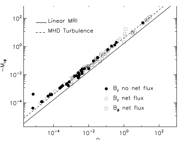
Figure 3: The correlation between the Maxwell stress, $\bar{M}_{r\phi}$, and the Reynolds stress, $\bar{R}_{r\phi}$, at saturation obtained in numerical simulations of shearing boxes with Keplerian velocity profiles but different initial conditions. Filled circles correspond to simulations with zero net vertical magnetic flux. Open circles correspond to simulations with finite net vertical magnetic flux. Squares correspond to simulations with an initial toroidal field. (See the text for references.) The dashed line is the correlation often quoted in the literature. The solid line corresponds to the late-time ratio of the two stresses during the exponential growth of the MRI, as predicted by equation (66) for $q=3/2$.

The dependence of the ratio of the stresses on the shear parameter, $q$, has not been studied extensively with numerical simulations so far. The only comprehensive study is by Hawley, Balbus, & Winters (1999) and their result is shown in Figure 4 . Superimposed on the figure is the analytic prediction, equation (66), for the ratio of the stresses as a function of the shear $q$ at late times during the exponential growth of the MRI. In this case, the qualitative trend followed by the ratio of the stresses at saturation as a function of the shear parameter $q$ seems also to be similar to that obtained at late times during the linear phase of the instability.

Figure 4: The dependence of the ratio of the mean Maxwell to the mean Reynolds stresses, $-\bar{M}_{r\phi}/\bar{R}_{r\phi}$, on the shear parameter $q$. The data points correspond to the results of shearing box simulations by Hawley, Balbus, & Winters (1999) in the saturated state. The solid line shows the analytic result (eq. [66]) for the ratio of the mean stresses during the late time of the exponential growth of the MRI.

The simultaneous analysis of Figures 3 and 4 demonstrates that the ratio $-\bar{M}_{r\phi}/\bar{R}_{r\phi}$ during the turbulent saturated state in local simulations of accretion discs is determined almost entirely by the local shear and depends very weakly on the other properties of the flow or the initial conditions. These figures also show that the ratios of the Maxwell to the Reynolds stresses calculated during the turbulent saturated state are qualitatively similar to the corresponding ratios found during the late times of the linear phase of the instability, even though the latter are slightly lower (typically by a factor of 2). This is remarkable because, when deriving equation (66) we have assumed that the MHD fluid is incompressible and considered only fluctuations that depend on the vertical, $z$, coordinate. Moreover, in the spirit of the linear analysis, we have not incorporated energy cascades between different scales, neither did we consider dissipation or reconnection processes that lead to saturation. Of course, the numerical simulations addressing the non-linear regime of the instability do not suffer from any of the approximations invoked to solve for the temporal evolution of the stresses during the phase of exponential growth. Nevertheless, the ratio of the Maxwell to the Reynolds stresses that characterize the turbulent saturated state are similar (to within factors of order unity) to the ratios characterizing the late times of the linear phase of the instability.

Appendix A Mean Values of Correlation Functions

For convenience, we provide here a brief demonstration of equation (49). The relationship between the mean value of the product of two real functions, $\overline{fg}$, and their corresponding Fourier transforms can be obtained by substituting the expressions for $f(z,t)$ and $g(z,t)$ in terms of their Fourier series, i.e.,

$$f(z,t)\equiv\sum_{n=-\infty}^{\infty}\hat{f}(k_{n},t)\,e^{ik_{n}z}\,,$$ (67)

into the expression for the mean value,

$$\overline{fg}\,(t)\equiv\frac{1}{2H}\int_{-H}^{H}f(z,t)\,g(t,z)\,dz\,.$$ (68)

The result is,

$$\overline{fg}\,(t)=\!\!\!\sum_{n,m=-\infty}^{\infty}\!\!\!\hat{f}(k_{n},t)\,\hat{g}^{*}(k_{m},t)\,\frac{1}{2H}\int_{-H}^{H}\!\!\!e^{i(k_{n}-k_{m})z}\,dz\,,$$ (69)

which can be rewritten using the orthogonality of the Fourier polynomials in the interval $[-H,H]$ as

$$\overline{fg}\,(t)=\sum_{n=-\infty}^{\infty}\hat{f}(k_{n},t)\hat{g}^{*}(k_{n},t)\,.$$ (70)

This is the discrete version of Plancherel’s theorem which states that the Fourier transform is an isometry, i.e., it preserves the inner product (see., e.g., Shilov & Silverman, 1973).

Denoting the Fourier transforms $\hat{f}(k_{n},t)$ and $\hat{g}^{*}(k_{n},t)$ by $\hat{f}_{n}$ and $\hat{g}^{*}_{n}$ in order to simplify the notation, we can write the following series of identities

$$\overline{fg}\,(t) = \sum_{n=-\infty}^{\infty}\hat{f}_{n}\hat{g}^{*}_{n}\,,$$ (71)

$$= \hat{f}_{0}\,\hat{g}_{0}+\sum_{n=1}^{\infty}\hat{f}_{n}\hat{g}^{*}_{n}+\sum_{n=-\infty}^{-1}\hat{f}_{n}\hat{g}^{*}_{n}$$ (72)

$$= \hat{f}_{0}\,\hat{g}_{0}+\sum_{n=1}^{\infty}\left[\hat{f}_{n}\hat{g}^{*}_{n}+\hat{f}_{-n}\hat{g}^{*}_{-n}\right]$$ (73)

$$= \hat{f}_{0}\,\hat{g}_{0}+\sum_{n=1}^{\infty}\left[\hat{f}_{n}\hat{g}_{n}^{*}+\hat{f}_{n}^{*}\hat{g}_{n}\right]$$ (74)

$$= \hat{f}_{0}\,\hat{g}_{0}+2\sum_{n=1}^{\infty}\;{\rm Re}[\hat{f}_{n}\hat{g}_{n}^{*}]\,,$$ (75)

where we have used the fact that the functions $f(z,t)$ and $g(z,t)$ are real and, hence, their Fourier transforms satisfy $\hat{f}_{-n}=\hat{f}^{*}_{n}$ and $\hat{g}_{-n}=\hat{g}^{*}_{n}$. Note that the factors $\hat{f}_{0}$ and $\hat{g}_{0}$ are just the mean values of the functions $f(z,t)$ and $g(z,t)$ and, therefore, do not contribute to the final expression in equation (49). It is then clear that, no matter whether the initial Fourier transforms corresponding to the functions $f(z,t)$ and $g(z,t)$ are real or imaginary, the mean value, $\overline{fg}\,(t)$, will be well defined.

Appendix B Energetics of MRI-driven Fluctuations

The relationships given in equation (36) lead to identities and inequalities involving the different mean stress components and the mean kinetic and magnetic energies associated with the fluctuations. In particular, the total mean stress is bounded by the total mean energy of the fluctuations. Moreover, the ratio of the mean magnetic to the mean kinetic energies is equal to the (absolute value of the) ratio between the mean Maxwell and the mean Reynolds stresses given by equation (66).

As we defined the mean stresses in terms of their per-$k$ contributions in §4, we can also define, to leading order in time, the mean energies associated with the fluctuations in the velocity and magnetic field by

$$\bar{E}_{K}(t)=2\sum_{n=1}^{k_{\mathrm{BH}}}\mathcal{E}_{K}(k_{n})\,|a_{1}|^{2}e^{2\gamma t}\,,$$ (76)

$$\bar{E}_{M}(t)=2\sum_{n=1}^{k_{\mathrm{BH}}}\mathcal{E}_{M}(k_{n})\,|a_{1}|^{2}e^{2\gamma t}\,,$$ (77)

where the corresponding per-$k$ contributions are given by

$$\mathcal{E}_{K}(k_{n}) = \frac{1}{2}\,[\mathcal{R}_{rr}(k_{n})+\mathcal{R}_{\phi\phi}(k_{n})]\,,$$ (78)

$$\mathcal{E}_{M}(k_{n}) = \frac{1}{2}\,[\mathcal{M}_{rr}(k_{n})+\mathcal{M}_{\phi\phi}(k_{n})]\,.$$ (79)

Figure 2 shows the dependences of the functions $\mathcal{E}_{K}(k_{n})$ and $\mathcal{E}_{M}(k_{n})$ for a Keplerian profile, $q=3/2$, and illustrates the fact that $\mathcal{E}_{M}(k_{n})>\mathcal{E}_{K}(k_{n})$ for $0<k_{n}<k_{\rm BH}$ and $0<q<2$.

Using equation (36) and the expression for the dispersion relation (23), it is easy to show that the following inequalities hold for each wavenumber $k_{n}$

$$\frac{\mathcal{R}_{r\phi}(k_{n})}{\mathcal{E}_{K}(k_{n})}=\frac{-\mathcal{M}_{r\phi}(k_{n})}{\,\,\mathcal{E}_{M}(k_{n})}=\frac{2\gamma(k_{n})}{q}\leq 1\,,$$ (80)

as long as $q>0$. It immediately follows that the same inequalities are also satisfied by the corresponding means, i.e.,

$$\bar{R}_{r\phi}(t) \leq \bar{E}_{K}(t)\,,$$ (81)

$$-\bar{M}_{r\phi}(t) \leq \bar{E}_{M}(t)\,.$$ (82)

This result, in turn, implies that the total mean energy associated with the fluctuations, $\bar{E}(t)=\bar{E}_{K}(t)+\bar{E}_{M}(t)$, sets an upper bound on the total mean stress, i.e.,

$$\bar{T}_{r\phi}(t)\leq\bar{E}(t)\,.$$ (83)

At late times during the exponential growth of the instability, the growth of the fluctuations is dominated by the mode with $k_{n}=k_{\max}$ and the mean stress $\bar{T}_{r\phi}(t)$ will tend to the total mean energy $\bar{E}(t)$, i.e.,

$$\lim_{t\gg 1}\bar{T}_{r\phi}(t)=\lim_{t\gg 1}\bar{E}(t)\,.$$ (84)

Furthermore, according to the first equality in equation (80), we can conclude that the ratio of the mean magnetic to the mean kinetic energies has the same functional dependence on the shear parameter, $q$, as does the (negative of the) ratio between the mean Maxwell and the mean Reynolds stresses given by equation (66), i.e.,

$$\lim_{t\gg 1}\frac{\bar{E}_{M}(t)}{\bar{E}_{K}(t)}=\frac{4-q}{q}\,.$$ (85)

Therefore, the mean energy associated with magnetic fluctuations is always larger than the mean energy corresponding to kinetic fluctuations as long as the flow is Rayleigh-stable.

References

- Balbus (2003) Balbus S.A., 2003, ARA&A, 41, 555
- Balbus & Hawley (1991) Balbus S.A., Hawley J.F., 1991, ApJ, 376, 214
- Balbus & Hawley (1992) Balbus S.A., Hawley J.F., 1992, ApJ, 392, 662
- Balbus & Hawley (1998) Balbus S.A., Hawley J.F., 1998, Rev. Mod. Phys., 70, 1
- Balbus & Hawley (2002) Balbus S.A., Hawley J.F., 2002, ApJ, 573, 749
- Balbus & Papaloizou (1999) Balbus S.A., Papaloizou J.C.B., 1999, ApJ, 521, 650
- Brandenburg & Campbell (1997) Brandenburg A., Campbell C., Accretion Disks - New Aspects, Proceedings of the EARA Workshop Held in Garching, Germany, 21-23 October 1996, XIII. Springer-Verlag, Berlin
- Brandenburg, Nordlund, Stein, & Torkelsson (1995) Brandenburg, A., Nordlund, A., Stein, R.F.; Torkelsson, U., 1995, ApJ, 446, 741
- Brandenburg (2001) Brandenburg A., 2001, ApJ, 550, 824
- Fleming & Stone (2003) Fleming T., Stone J.M., 2003, ApJ, 585, 908
- Gardiner & Stone (2005) Gardiner T., Stone, J.M., 2005, in Magnetic Fields in the Universe, AIP Conf. Proc., 784, 475
- Goodman & Xu (1994) Goodman J., Xu G., 1994, ApJ, 432, 213
- Hawley, Gammie, & Balbus (1995) Hawley J.F., Gammie C.F., Balbus S.A., 1995, ApJ, 440, 742
- Hawley, Gammie, & Balbus (1996) Hawley J.F., Gammie C.F., Balbus S.A., 1996, ApJ, 464, 690
- Hawley, Balbus, & Winters (1999) Hawley J.F., Balbus S.A., Winters W.F., 1999, ApJ, 518, 394
- Hawley (2000) Hawley J.F., 2000, ApJ, 528, 462
- Hawley (2001) Hawley J.F., 2001, ApJ, 554, 534
- Hoffman & Kunze (1971) Hoffman K.M., Kunze R., 1971, Linear Algebra, 2nd ed. Prentice Hall, N.J.
- Kato, Fukue, & Mineshige (1998) Kato S., Fukue J., Mineshige S., 1998, Black-Hole Accretion Disks. Kyoto University Press., Kyoto
- Narayan, Quataert, Igumenshchev, & Abramowicz (2002) Narayan R., Quataert E., Igumenshchev I.V., Abramowicz M.A., 2002, ApJ, 577, 295
- Sano, Inutsuka, Turner, & Stone (2004) Sano T., Inutsuka S., Turner N.J., Stone J.M., 2004, ApJ, 605, 321
- Shakura & Sunyaev (1973) Shakura N.I., Sunyaev R.A., 1973, A&A, 24, 337
- Shilov & Silverman (1973) Shilov G.E., Silverman R.A., 1973, Mathematical Analysis. MIT Press, Cambridge
- Stone & Pringle (2001) Stone J.M., Pringle J.E., 2001, MNRAS, 322, 461
- Stone, Hawley, Gammie, & Balbus (1996) Stone J.M., Hawley J.F., Gammie C.F., Balbus S.A., 1996, ApJ, 463, 656