The DEEP2 Galaxy Redshift Survey: The Relationship between Galaxy Properties and Environment at $z\sim 1$

Abstract

We study the mean environment of galaxies in the DEEP2 Galaxy Redshift Survey as a function of rest-frame color, luminosity, and [OII] 3727Å equivalent width. The local galaxy overdensity for $>\!14,000$ galaxies at $0.75<z<1.35$ is estimated using the projected $3^{\rm rd}$-nearest-neighbor surface density. Of the galaxy properties studied, mean environment is found to depend most strongly on galaxy color; all major features of the correlation between mean overdensity and rest-frame color observed in the local universe were already in place at $z\sim 1$. In contrast to local results, we find a substantial slope in the mean dependence of environment on luminosity for blue, star-forming galaxies at $z\sim 1$, with brighter blue galaxies being found on average in regions of greater overdensity. We discuss the roles of galaxy clusters and groups in establishing the observed correlations between environment and galaxy properties at high redshift, and we also explore the evidence for a “downsizing of quenching” from $z\sim 1$ to $z\sim 0$. Our results add weight to existing evidence that the mechanism(s) that result in star-formation quenching are efficient in group environments as well as clusters. This work is the first of its kind at high redshift and represents the first in a series of papers addressing the role of environment in galaxy formation at $0<z<1$.

1. Introduction

For more than a few decades now, the observed properties of galaxies have been known to depend upon the environment in which they are located. For instance, elliptical and lenticular galaxies are systematically over-represented in highly overdense environments such as galaxy clusters (e.g. Davis & Geller, 1976; Dressler, 1980; Postman & Geller, 1984; Balogh et al., 1998). Similarly, measurements of the 2-point galaxy correlation function for different luminosity and color subpopulations have provided a complementary window to what galaxies populate different environments (Zehavi et al., 2002; Norberg et al., 2002; Madgwick et al., 2003; Coil et al., 2004b). Furthermore, recent studies utilizing the Sloan Digital Sky Survey (York et al., 2000, SDSS) and the 2-degree Field Galaxy Redshift Survey (Colless et al., 2001, 2dFGRS) have found that a wide array of galaxy properties (e.g. color, luminosity, surface-brightness, star-formation rate, and AGN activity) correlate with the local density of the galaxy environment and that the observed correlations extend from the centers of clusters out into the field galaxy population (Lewis et al., 2002; Gómez et al., 2003; Balogh et al., 2004a; Hogg et al., 2004; Christlein & Zabludoff, 2005).

Current hierarchical galaxy formation models predict that galaxies form in less dense environments and are then accreted into larger groups and clusters (Kauffmann et al., 1993; Somerville & Primack, 1999; Cole et al., 2000; De Lucia et al., 2005). Within such models, there are a plethora of physical processes that could explain the observed trends with environment. For example, galaxy mergers, which preferentially occur in galaxy groups rather than clusters (e.g. Cavaliere et al., 1992), can destroy galactic disks and thereby convert spiral galaxies into ellipticals and lenticulars (Toomre & Toomre 1972); likewise, ram-pressure stripping within galaxy clusters can effectively suffocate star formation in member galaxies (Gunn & Gott 1972), and within overdense regions galaxies can be swept of their gas via feedback from AGN, thus quenching the star-formation process (Springel et al., 2005).

In recent years, many studies have focused on measuring the correlations between galaxy properties and environment at $z\sim 0$. For example, using large data sets from local surveys such as the SDSS, Blanton et al. (2004), Kauffmann et al. (2004), Croton et al. (2005b) measured the relationship between star-formation history and local galaxy density for environments ranging from voids to clusters. At high redshift, however, such analysis over a similar environment range and with a comparable sample size has yet to be completed due in large part to the lack of a suitable data set. While studies of clusters have pushed to high redshift, the range of environments probed in such studies has been limited, with galaxies grouped into coarse classifications (such as field, group, and cluster populations) and with statistically small spectroscopic sample sizes (e.g., Couch et al., 1998; Treu et al., 2003; Smith et al., 2005; Tanaka et al., 2005; Poggianti et al., 2005). As discussed by Cooper et al. (2005), to measure galaxy environments accurately at $z\sim 1$, a survey must obtain high-precision (i.e. spectroscopic) redshifts over a large and contiguous field with a relatively high sampling rate. The DEEP2 Galaxy Redshift Survey (Davis et al., 2003; Faber et al., 2006) is the first survey at high redshift to provide such a sample, opening the door to studying galaxy properties and environments at $z\sim 1$ over a continuous range of environments from voids to large groups.

Studying the relationship between environment and galaxy properties at high redshift should afford the perspective needed to understand the nature of the observed relations found locally. In particular, studying galaxy environments at higher $z$ will help determine whether the correlations observed in the nearby universe are a result of evolutionary processes with long time-scales or whether the observed relations were in place very early in the lifetime of the universe. Constraints derived from $z\sim 1$ studies should also yield information regarding the physical processes (e.g. ram-pressure stripping, harassment, and mergers) and possible environment regimes (e.g. groups versus clusters) that are significant in creating the trends seen locally.

In this paper, we study the environment of high-redshift $(z\sim 1)$ galaxies in the DEEP2 Galaxy Redshift Survey with a goal of determining the correlation between local density and galaxy properties when the universe was half its present age. In particular, we examine the relations between environment and galaxy color, luminosity, and [OII] equivalent width. In §2, we describe the DEEP2 survey and the galaxy sample under study. The measurements of galaxy properties including color, luminosity, [OII] equivalent width, and local density are dicussed in §3 and §4. In §5, we present our results and a qualitative comparison to observations at $z\sim 0$. Lastly, in §6 we summarize and discuss our findings with some additional discussion directed towards future analysis utilizing the DEEP2 survey. Throughout this paper, we employ a $\Lambda$CDM cosmology with $w=-1$, $\Omega_{M}=0.3$, $\Omega_{\Lambda}=0.7$, and $h=1$.

2. Data Sample

The DEEP2 Galaxy Redshift Survey (Davis et al., 2003; Faber et al., 2006) is an ongoing project designed to study the galaxy population and large-scale structure at $z\sim 1$. The survey utilizes the DEIMOS spectrograph (Faber et al., 2003) on the 10-meter Keck II telescope to target $\gtrsim\!40,000$ galaxies covering $\sim 3$ square degrees of sky over four widely separated fields. In each field, targeted galaxies are selected to $R_{\rm AB}\leq 24.1$ from deep $B,R,I$ imaging taken with the CFH12k camera on the 3.6-meter Canada-France-Hawaii Telescope (Coil et al., 2004a; Davis et al., 2004). Using a simple color-cut in three of the survey fields, the high-redshift $(z>0.7)$ galaxies are selected for observation with only $\lesssim\!3\%$ of galaxies at $z>0.75$ rejected, based on tests in the fourth survey field, the Extended Groth Strip (Davis et al., 2004; Faber et al., 2006).

This work utilizes data from the first six DEEP2 observing seasons (collected from August 2002 – July 2005) spread over three of the survey’s four fields. The DEIMOS data were processed using a sophisticated IDL pipeline, developed at UC-Berkeley (Cooper et al., 2006b) and adapted from spectoscopic reduction programs created for the SDSS (Burles & Schlegel, 2006). The observed spectra were taken at moderately high spectral resolution $(R\sim 5000)$ and typically span an observed wavelength range of $6300{\rm\AA}\ <\lambda<9100{\rm\AA}$. Working at such high resolution, we are able to unambigously detect and resolve the [OII] 3727Å doublet for galaxies in the redshift range $0.7<z<1.4$. Absorption-based redshifts are also measured, primarily relying upon the Ca H and Ca K features which are detectable out to redshifts of $z\sim 1.3$. Repeated observations of a subset of galaxies yield an effective velocity uncertainty of $\sim\!30\ {\rm km}/{\rm s}$ due to differences in the position or alignment of a galaxy within a slit or internal kinematics within a galaxy (Faber et al., 2006).

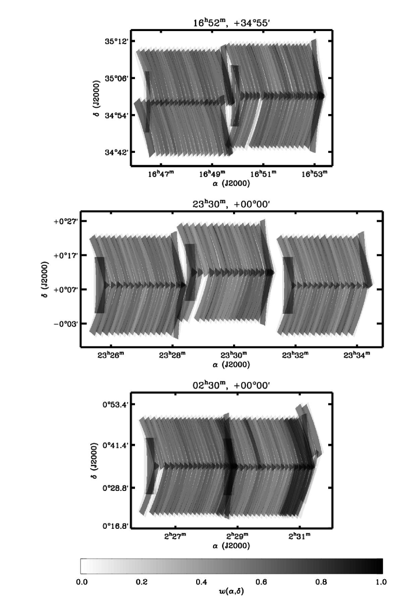
Figure 1.— We present the 2-d redshift completeness map, $w(\alpha,\delta)$, for spectroscopic coverage in each survey field. We include all 280 slitmasks with redshift completeness for red $({\rm observed}\ R-I>0.5)$ galaxies $\geq 65\%$ in our analysis. The greyscale in each image ranges from 0 (white) to 0.95 (black) and corresponds to the probability that a galaxy meeting the survey selection criteria at that position on the sky was targeted for spectroscopy and a redshift was successfully measured. The color bar at the bottom shows the value of $w(\alpha,\delta)$ as function of the greyscale.

We present results from the most complete portions of three of the DEEP2 fields. The data sample spans 280 DEIMOS slitmasks, covering a total of $\gtrsim\!2\ {\rm degrees}^{2}$ of sky with an average redshift completeness of $\gtrsim 70\%$. We use data only from slitmasks which have a redshift success rate of 65% or higher for red $(R-I>0.5)$ galaxies in order to avoid systematic effects which may bias our results. The success rate for red galaxies is well correlated with the signal-to-noise of the 1-d spectra on a slitmask, with a roughly Gaussian distribution of redshift completeness (that is, success rate) above 65%, with a mean of $\sim 80\%$. Figure 1 shows the 2-dimensional redshift completeness map for each of the surveyed fields. The completeness map gives the probability at that position on the sky that a galaxy meeting the survey selection criteria was targeted for spectroscopy and a redshift was successfully measured. The total data sample (Sample A in Table 1) in the three fields includes 22,416 sources with accurate redshift determinations (quality $Q=3$ or $Q=4$ as defined by Faber et al., 2006) within the redshift range $0.2<z<2$; we show the redshift distribution of this sample in Figure 2.

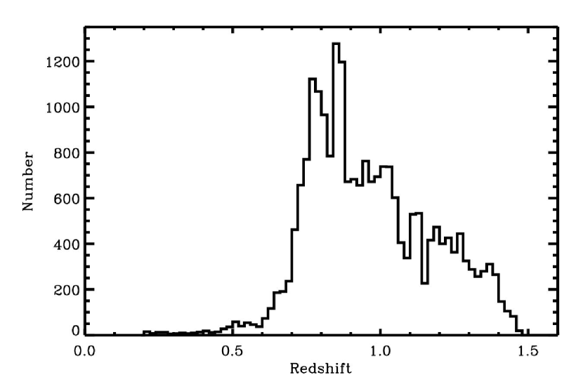
Figure 2.— The observed redshift distribution for all 23,004 sources in the three surveyed regions. The color cut rejects $\lesssim 3\%$ of galaxies with $z>0.75$, based on tests in the Extended Groth Strip (Faber et al., 2006). The redshift histogram is plotted using a bin size of $\Delta z=0.02$.

3. Measurements of Galaxy Properties

In this section, we describe the set of galaxy properties for which we study the distributions and correlations with local environment. The properties to be discussed include galaxy color, luminosity, and [OII] equivalent width. In the following subsections, we detail the measurement of each property within the DEEP2 sample.

3.1. Galaxy Colors and Luminosities

The rest-frame color, $(U-B)_{0}$, and absolute $B$-band magnitude, $M_{B}$, are calculated by combining the CFHT $B,R,I$ photometry with spectral energy distributions (SEDs) of galaxies ranging from 1180Å to 10000Å as compiled by Kinney et al. (1996). By projecting the Kinney et al. (1996) SEDs onto the response functions for the CFHT filters and for the corresponding standard Johnson filters (Bessell, 1990), we compute the rest-frame $U-B$ and $B-R_{\rm cfht}$ colors, the ${\rm K}_{R_{\rm cfht}}$ transformations, and the expected observed colors for each SED at the redshift of the galaxy for which we are correcting. A low-order polynomial is then fit between the synthetic $B_{\rm cfht}-R_{\rm cfht}$, $R_{\rm cfht}-I_{\rm cfht}$ colors and the $U-B$ color and $B-R_{\rm cfht}-{\rm K}_{R_{\rm cfht}}$ transformation. By using the coefficients of the fit, the final rest-frame color and absolute magnitude for each galaxy are calculated in the Johnson filter set. In computing the K-corrections, we follow the notation of Hogg et al. (2002). For all details regarding the DEEP2 photometric catalog and measured source fluxes, refer to Coil et al. (2004a). For specifics relating to the computation of rest-frame colors and luminosities, refer to Willmer et al. (2005). Unless explicitly stated otherwise, all magnitudes discussed in this paper are given in AB magnitudes (Oke & Gunn, 1983). For zero-point conversions between AB and Vega magnitudes, refer to Table 1 of Willmer et al. (2005).

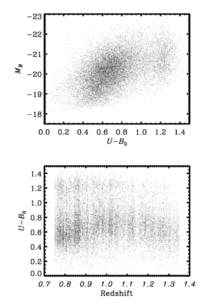
Figure 3.— (Top) Plotted is the color-magnitude relation for the 18,977 sources in the sample within the redshift range $0.75<z<1.35$ (Sample B in Table 1). (Bottom) We plot the rest-frame $(U-B)_{0}$ color distribution with redshift for the same sample. At high redshift $(z>1.1)$, the red galaxy fraction drops significantly due primarily to the $R_{\rm AB}$ magnitude limit of the survey (Willmer et al., 2005).

Figure 3 shows the color-magnitude relation for the 18,977 galaxies at $0.75<z<1.35$ in the data sample. A distinct bimodality exists in the color distribution with a division at $(U-B)_{0}\sim 1.0$, separating members of the “blue cloud” from red-sequence galaxies (e.g. Strateva et al., 2001; Baldry et al., 2004; Bell et al., 2004; Weiner et al., 2005). Within the DEEP2 sample, the division between the red and blue populations shows little sign of evolution (Willmer et al., 2005); as illustrated in Figure 3, over the entire redshift range probed in the data set, a strong division is observed at $(U-B)_{0}\sim 1.0$. However, at redshifts beyond $z\sim 1.1$, the red galaxy fraction decreases precipitously in the DEEP2 sample, due to the survey’s $R$-band magnitude limit. For a more thorough discussion of rest-frame colors and luminosities in the DEEP2 survey, we direct the reader to Willmer et al. (2005).

3.2. [OII] Equivalent Widths

For each object in the sample, we measure the equivalent width of the [OII] 3727Å doublet if it is within the wavelength coverage of the observed spectrum. We utilize the boxcar-extracted 1-D spectrum and errors produced by the DEEP2 pipeline (Cooper et al., 2006b; Faber et al., 2006) and fit a double Gaussian profile to the wavelength, flux, and error of pixels in a 40Å window centered on the predicted location of the [OII] emission. The fit uses a Levenberg-Marquardt nonlinear least squares minimization routine (Press et al., 1992) with the following free parameters: continuum, intensity, central wavelength, dispersion, and intensity ratio of the two lines in the [OII] doublet. This routine produces best-fit values and error estimates. In fitting the Gaussian profiles, the wavelength ratio of the two lines in the doublet is fixed, but the intensity ratio is allowed to vary. The fitted continuum is noisy when the data have low S/N, so we make a robust estimate of the continuum by taking the biweight (Beers et al., 1990) of all data in two windows on either side of the line, each 80Å long and separated from the line by a 20Å buffer. The rest-frame [OII] equivalent width and error are derived from the total intensity of the doublet and the robust continuum. For all analysis utilizing [OII] equivalent widths, we limit the sample studied to those galaxies for which the uncertainty in $W_{\rm[OII]}$ is small $(\sigma_{W_{\rm[OII]}}<10\ {\rm\AA})$, a selection that retains $\sim 45\%$ of galaxies.

4. Local Galaxy Densities

For each galaxy in the data set, we estimate the local galaxy density using the projected $3^{\rm rd}$-nearest-neighbor surface density, $\Sigma_{3}$. In computing $\Sigma_{3}$, the full DEEP2 galaxy sample is employed and we utilize a velocity interval of $\pm 1000\ {\rm km}/{\rm s}$ along the line-of-sight to exclude foreground and background galaxies. The measured surface density depends on the projected distance to the $3^{\rm rd}$-nearest neighbor, $D_{p,3}$, as $\Sigma_{3}=3/\left(\pi D_{p,3}^{2}\right)$, such that $\Sigma_{3}=0.1\ {\rm galaxies}/{(h^{-1}{\rm comovingMpc})^{2}}$ corresponds to a projected $3^{\rm rd}$-nearest-neighbor distance of $\sim 3\ h^{-1}$ comoving Mpc and surface density of unity corresponds to a length scale of $D_{p,3}\sim 1\ h^{-1}$ comoving Mpc. From tests using the mock galaxy catalogs of Yan et al. (2004), Cooper et al. (2005) find the projected $3^{\rm rd}$-nearest-neighbor distance to be a robust and accurate environment measure that minimizes the role of redshift-space distortions and edge effects. Further details regarding the computation and sensitivity of this density measure as well as comparisons to other common environment estimators are presented in Cooper et al. (2005).

4.1. Correcting for Variations in Redshift Sampling and Completeness

To correct each density estimate for the variable redshift completeness of the DEEP2 survey, we scale the density measured about each galaxy according to the local value of the 2-dimensional survey completeness map, $w(\alpha,\delta)$, which accounts for variations in targeting rate and redshift completeness from position to position within the survey (Coil et al., 2004b). Each density value is also corrected for the redshift dependence of the sampling rate of the survey using the empirical method presented in Cooper et al. (2005): each density value is divided by the median $\Sigma_{3}$ of galaxies at that redshift over the whole sample, where the median is computed in bins of $\Delta z=0.04$. Using mock galaxy catalogs, Cooper et al. (2005) conclude that such an empirical correction is effective at reducing the influence of variations in redshift sampling in the survey without overcorrecting variations in enviroment due to cosmic variance. Correcting the measured densities in this manner converts the $\Sigma_{3}$ values into measures of overdensity relative to the median density $({\rm denoted}\ {\rm by}\ 1+\delta_{3})$, and is similar to the methods employed by Hogg et al. (2003) and Blanton et al. (2004). To ensure that the applied corrections are not exceedingly large, we restrict the analysis presented in this paper to galaxies in the redshift interval $0.75<z<1.35$, where the DEEP2 selection function is relatively shallow.

4.2. Edge Effects

When calculating the local density of galaxies, the confined sky coverage of a survey introduces geometric distortions – or edge effects – which bias environment measures near edges or holes in the survey field, generally causing densities to be under-estimated (Cooper et al., 2005). We define the DEEP2 survey area and corresponding edges according to the 2-dimensional survey completeness map and the photometric bad-pixel mask used in slitmask design – defining all regions of sky with $w(\alpha,\delta)<0.35$ averaged over scales of $\gtrsim 30^{\prime\prime}$ to be unobserved and rejecting all significant regions of sky ($\gtrsim 30^{\prime\prime}$ in scale) which are incomplete in the photometric catalog. Areas of incompleteness on scales $\lesssim 30^{\prime\prime}$ are comparable to the typical angular separation of galaxies targeted by DEEP2 (Gerke et al., 2005; Cooper et al., 2005), and thus cause a negligible perturbation to the measured densities.

To minimize the impact of edges on the data sample, we exclude any galaxy within $1\ h^{-1}$ comoving Mpc of an edge or gap. Such a cut greatly reduces the portion of the data set contaminated by edge effects (Cooper et al., 2005) while retaining $\sim\!75\%$ of the full galaxy sample. Combined with the restriction to the redshift regime $0.75<z<1.35$, this gives a final sample comprising 14,214 galaxies. For easy reference, the details regarding the galaxy samples utilized throughout this paper are listed in Table 1. The distribution of overdensities, $(1+\delta_{3})$, for this sample (Sample C in Table 1) is shown in Figure 4.

Figure 4.— In logarithmic space, we plot the distribution of local overdensities, $(1+\delta_{3})$, for the 14,214 galaxies with $0.75<z<1.35$ and more than $1\ h^{-1}$ comoving Mpc from a survey edge, comprising the Sample C (see Table 1) for this paper (solid line). We also show the distribution of overdensities for galaxies in groups and clusters as identified by Gerke et al. (2005). The dotted line gives the distribution of $\log_{10}{(1+\delta_{3})}$ for all galaxies in groups or clusters and the dashed line gives the distribution for galaxies in groups or clusters with a velocity dispersion $\sigma_{\rm group}>200\ {\rm km}/{\rm s}$ as measured by Gerke et al. (2005). The overdensity, $(1+\delta_{3})$, is a dimensionless quantity, computed as described in §4.1.

4.3. Target-Selection Effects

Due to the need to design DEIMOS slitmasks such that spectra do not overlap and due to the adopted target-selection and slitmask-tiling schemes of the survey, the DEEP2 survey slightly under-samples projected overdensities of galaxies on the sky (Gerke et al., 2005; Cooper et al., 2005). Such a bias in the survey is a critical concern for the measurement of accurate galaxy densities in highly-clustered environments. However, using the mock catalogs of Yan et al. (2004) to test the survey target-selection and slitmask-making procedures, Cooper et al. (2005) find that while the DEEP2 survey under-samples dense regions of sky (projected densities on the sky), the survey does not under-sample dense environments (that is, local densities in three-dimensional space) to any significant degree.

4.4. Measurement Errors

We have determined the uncertainty in our environment measures using the mock galaxy catalogs of Yan et al. (2004). In order to simulate the DEEP2 sample, the volume-limited mock catalogs are passed through the DEEP2 target-selection and slitmask-making procedures as described by Davis et al. (2004) and Faber et al. (2006), placing $\sim 60\%$ of targets on a slitmask. Using the same techniques as applied to the data, we measure the environment for each galaxy in the simulated DEEP2 sample. For each mock galaxy, this “observed” environment is compared to the “true” environment as measured in the full volume-limited catalog using the real-space positions for all of the galaxies. Measuring the scatter in “true” minus “observed” environment for the simulated DEEP2 galaxies shows a 1-$\sigma$ scatter of roughly 0.5 in units of $\log{(1+\delta_{3})}$. The uncertainty in the overdensity values shows little dependence on environment, with only a slight increase in the errors at higher densities. For more details on the mock catalogs or tests of environment measures using them, refer to Yan et al. (2004) and Cooper et al. (2005), respectively.

5. Results

The local density of galaxies is thought to influence galaxy characteristics such as morphology and star-formation rate, and thus such galaxy properties are often studied as a function of enviroment. Analyses performed in this manner are particularly helpful at recognizing scales or densities at which galaxy properties transition and are therefore useful in understanding the physical processes at play. Measurements of galaxy environment, however, are significantly more uncertain than measures of other properties such as color or luminosity. Therefore, by binning galaxies according to local density, there is a significant correlation between neighboring density bins which smears out any trends with other galaxy properties. Consequently, in this paper, we instead study the dependence of mean environment on galaxy properties. The mean relations are weighted according to the inverse selection volumes, $1/V_{\rm max}$; computing the mean in this manner minimizes the effects of Malmquist bias (Malmquist, 1936) in the sample. In computing the $1/V_{\rm max}$ values, we restrict the surveyed volume to $0.75<z<1.35$ and incorporate rest-frame color according to the K-corrections discussed in §3.1.

5.1. Dependence of Mean Environment on Galaxy Color

As shown in Figure 5, at $z\sim 1$, blue galaxies on average occupy less-dense environments. We observe a distinct transition in mean overdensity which corresponds well with the observed color bimodality. The mean environment for red galaxies at $z\sim 1$ is more than 1.5 times more dense than for their blue counterparts. At very blue colors, $(U-B)_{0}<0.3$, we also find significant evidence for a fall-off in the mean overdensity.

The observed relationship between galaxy overdensity and rest-frame color at $z\sim 1$ mirrors that seen in the local universe. The dependence of mean environment on color at $z\sim 0.1$ exhibits a strong transition in mean density occurring at the location of the color bimodality and a further decrease in mean density for the very bluest galaxies (Hogg et al., 2003; Blanton et al., 2003a; Balogh et al., 2004b). We find that this trend is already in place as early as a redshift of unity.

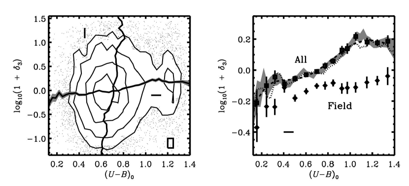
Figure 5.— (Left) We plot the logarithm of the local galaxy overdensity, $(1+\delta_{3})$, versus the rest-frame color, $(U-B)_{0}$, for all 14,214 galaxies in the $0.75<z<1.35$ sample (Sample C). The contours show the number density of sources as a function of $\log{(1+\delta_{3})}$ and $(U-B)_{0}$ and correspond to levels of 25, 50, 100, and 150 galaxies. The number density is computed in a sliding box of height $\Delta\log{(1+\delta_{3})}=0.2$ and width $\Delta(U-B)_{0}=0.05$ as illustrated in the lower right corner of the plot. The solid black horizontal line shows the weighted mean dependence of environment on color, while the vertical counterpart gives the weighted mean dependence of $(U-B)_{0}$ on environment. The respective means were computed using sliding boxes with widths given by the black dashes in the plot and were weighted according to the inverse selection volumes, $1/V_{\rm max}$. The accompanying grey regions correspond to the sliding 1-$\sigma$ uncertainties in the weighted means. (Right) We again show the 1-$\sigma$ region for the weighted mean dependence of environment on galaxy color computed in a sliding box of width given by the black dash (grey region). The square points and error bars give the weighted mean environments and 1-$\sigma$ uncertainties in the means computed in distinct bins of color, thereby avoiding the covariance associated with the sliding mean. The diamond points and error bars show the weighted mean environments and 1-$\sigma$ uncertainties in the means computed in indentical color bins for the field galaxy population solely. The field population is selected according to the galaxy group finder of Gerke et al. (2005), excluding all galaxies identified as group members. The dotted line shows the median $\log_{10}{(1+\delta_{3})}$ versus color trend utilizing the same sliding box. Lastly, a $6^{\rm th}$-order polynomial fit to the mean color dependence of galaxy environment is shown by the dashed line and used below (see Table 2 for coefficients of the fit). At $z\sim 1$, we find the relationship between rest-frame color and environment to echo the trend measured locally with red galaxies favoring regions of high overdensity and very blue objects preferrentially found in underdense environments.

As illustrated in Figure 3, the DEEP2 sample is heavily weighted towards blue galaxies at higher redshift; in addition, the sampling rate for DEEP2 decreases significantly beyond $z>1.1$ (see Fig. 2). The observed correlation between mean overdensity and color, however, is not a product of selection effects. By limiting the sample to $0.75<z<1.05$ and $M_{B}<-20$ where the red galaxy sample is complete and any evolution in the measured galaxy density is negligible, the observed color dependence of mean environment persists with the contrast in typical overdensity for red and blue galaxies unchanged relative to that observed for the full $0.75<z<1.35$ sample.

Using the group finder of Gerke et al. (2005), we are able to identify the set of galaxies within the data set not associated with groups or clusters, that is, the field population. In Figure 5, we show the mean dependence of environment on rest-frame $(U-B)_{0}$ color for this sub-population (diamond symbols). We find that among the field sample a weak trend with color exists such that red field members are found to be only slightly overdense relative to their blue conterparts. At very blue colors, however, the trend with mean overdensity is clearly evident within the field galaxy population.

5.2. Dependence of Mean Environment on [OII] Equivalent Width

As shown in Figure 6, the dependence of mean galaxy density on [OII] equivalent width, $W_{\rm[OII]}$, is a strong monotonic trend at $z\sim 1$. On average, galaxies with smaller equivalent widths occupy regions of higher density. Again, limiting the sample to galaxies in the redshift range $0.75<z<1.05$ and brighter than $M_{B}=-20$, we find the measured trend with $W_{\rm[OII]}$ to be essentiallly unchanged; we do not appear to be biased by any redshift dependence or selection effect in the sample.

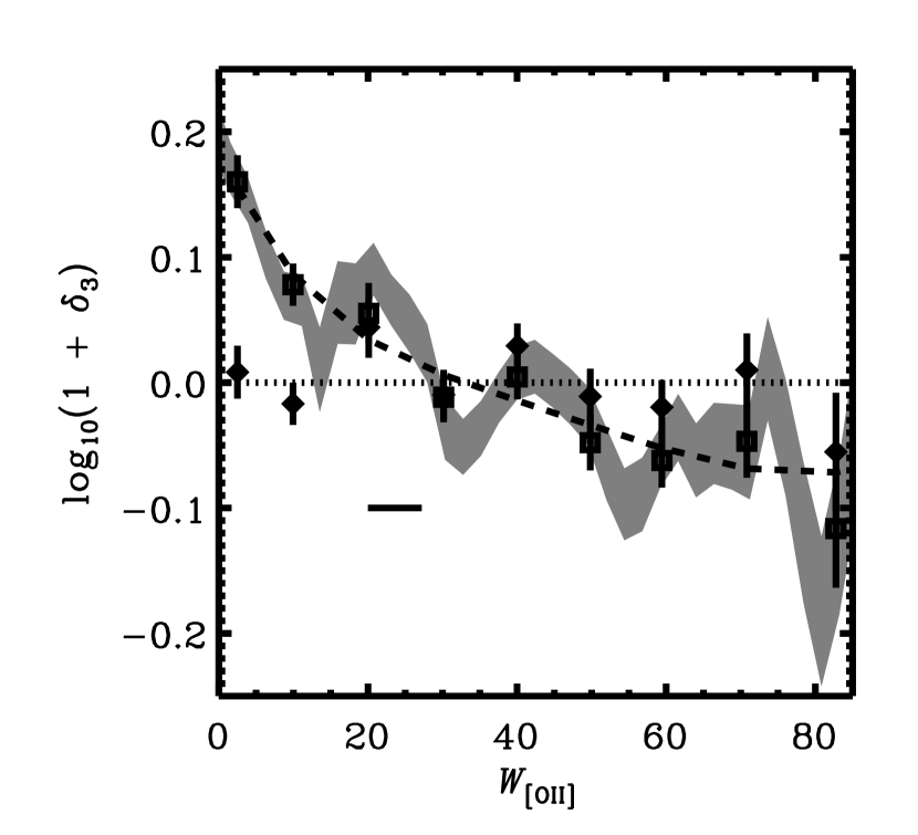
Figure 6.— We plot the mean relationship between the logarithm of the local galaxy overdensity, $(1+\delta_{3})$, and the measured [OII] equivalent width, $W_{\rm[OII]}$, for all 9,567 galaxies in the sample with $\sigma_{W_{\rm[OII]}}<10{\rm\AA}$ (Sample D). We compute the weighted mean dependence of environment on [OII] equivalent width, using a sliding box with width given by the black dash in the plot and weighted according to the inverse selection volumes, $1/V_{\rm max}$. The dashed line follows a $5^{\rm th}$-order polynomial fit to this mean dependence of environment on [OII] equivalent width. The plotted grey region corresponds to the sliding 1-$\sigma$ uncertainty in the weighted mean. The square points and error bars give the weighted mean environments and 1-$\sigma$ uncertainties in the means computed in distinct bins of $W_{\rm[OII]}$, thereby avoiding the covariance associated with the sliding mean. We fit a $6^{\rm th}$-order polynomial to the mean density relation with color (see Fig. 5) and subtract off this color dependence for each galaxy according to its rest-frame color. The diamond points and error bars show the weighted mean environments and 1-$\sigma$ uncertainties in the means computed in distinct bins of $W_{\rm[OII]}$ after the mean color dependence has been removed. We find a strong relationship between [OII] equivalent width and mean environment at $z\sim 1$, but we detect no additional dependence on $W_{\rm[OII]}$ separate from the dependence on rest-frame color.

The strength of the observed correspondence between environment and $W_{\rm[OII]}$ is not surprising given the close correlation between galaxy color and [OII] equivalent width, as shown in Figure 7 and found in previous studies of galaxy properties at $z\sim 1$ (e.g. Weiner et al., 2005). Red galaxies in the DEEP2 sample are strongly clustered in the $(U-B)_{0},W_{\rm[OII]}$ plane with $W_{\rm[OII]}<40{\rm\AA}$, while for the blue galaxy population [OII] equivalent width tends to increase rapidly with decreasing color. Fitting a $5^{\rm th}$-order polynomial to the mean overdensity relation with color (see Figure 5) and subtracting off this dependence for each galaxy according to its rest-frame color, we find no evidence for any residual environment dependence on [OII] equivalent width separate from the color dependence; the residual points in Figure 6 are consistent with a line of zero slope and intercept. Given the uncertainties in the measured quantities, simulations indicate that we would be able to detect a residual slope as small as $\sim\!0.3\log{(1+\delta_{3})}/{\rm\AA}$ equivalent width at a 3-$\sigma$ level. Conversely, if we apply this same test in reverse and check for residuals in mean environment with $(U-B)_{0}$ color when the trend between mean environment and $W_{\rm[OII]}$ has been removed, we find that a strong residual trend between $<\log_{10}{(1+\delta_{3})}>$ and $(U-B)_{0}$ does exist (see Fig. 8). That is, fitting to the dependence of mean overdensity on $W_{\rm[OII]}$ and subtracting off this dependence for each galaxy according to its [OII] equivalent width, we find a residual trend between mean environment and color.

This result suggests that [OII] equivalent width does not have a relationship with environment separate from that observed with rest-frame $(U-B)_{0}$ color. While both galaxy properties are indirect tracers of star-formation and local studies find a galaxy’s star-formation history to be strongly correlated with its environment (e.g. Blanton et al., 2003b), it is not suprising that galaxy color would be more closely correlated with galaxy environment. [OII] equivalent width more closely traces the instantaneous star-formation rate of a galaxy, which can be dictated by short-term processes such as minor mergers that are not inherently tied to the local density of bright galaxies on somewhat larger scales, which we measure in the DEEP2 data. Furthermore, $W_{\rm[OII]}$ is influenced by additional factors such AGN activity (Yan et al., 2005) which may further smear out the correlation between environment and star-formation as traced by $W_{\rm[OII]}$. Color, on the other hand, tracks the history of the galaxy on longer time-scales and as such may be more strongly correlated with the larger-scale environment of the galaxy as probed by the DEEP2 survey.

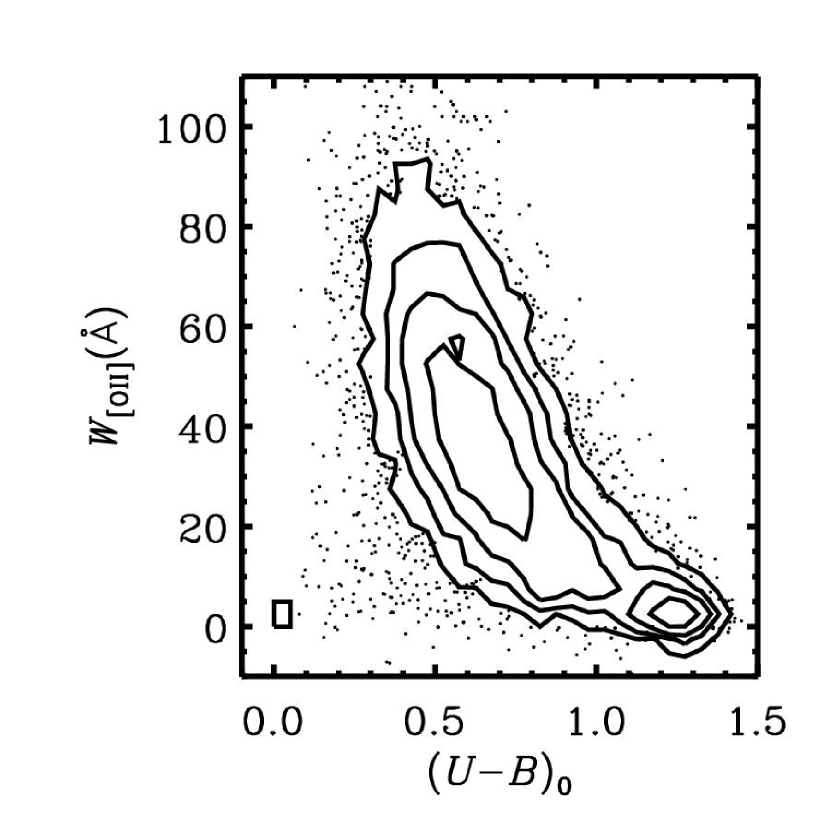
Figure 7.— The correlation between [OII] equivalent width, $W_{\rm[OII]}$, and rest-frame galaxy color, $(U-B)_{0}$, over the randshift range $0.75<z<1.35$. Here, we limit the sample plotted to those galaxies comprising Sample D of Table 1. The contours show the number density of sources as a function of $W_{\rm[OII]}$ and $(U-B)_{0}$ and correspond to levels of 10, 25, 50, and 100 galaxies. The number density is computed in a sliding box of height $\Delta W_{\rm[OII]}=5{\rm\AA}$ and width $\Delta(U-B)_{0}=0.05$ as illustrated in the lower left corner of the plot.

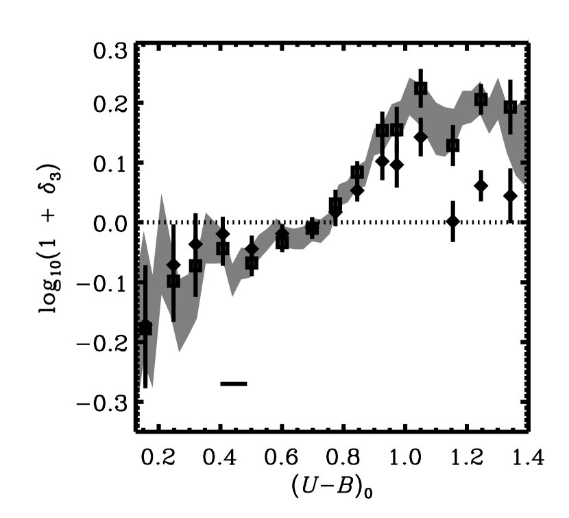
Figure 8.— We plot the relationship between the logarithm of the local galaxy overdensity, $(1+\delta_{3})$, and the rest-frame color, $(U-B)_{0}$ for all 9,567 galaxies in the sample with $\sigma_{W_{\rm[OII]}}<10{\rm\AA}$ (Sample D). We compute the weighted mean dependence of environment on color, using a sliding box with width given by the black dash in the plot and weighted according to the inverse selection volumes, $1/V_{\rm max}$. The plotted grey region corresponds to the sliding 1-$\sigma$ uncertainty in the weighted mean. The square points and error bars give the weighted mean environments and 1-$\sigma$ uncertainties in the means computed in distinct bins of $(U-B)_{0}$, thereby avoiding the covariance associated with the sliding mean. We fit a $5^{\rm th}$-order polynomial to the mean density relation with color (see Fig. 6 in the paper) and subtract off this color dependence for each galaxy according to its $W_{\rm[OII]}$. The diamond points and error bars show the weighted mean environments and 1-$\sigma$ uncertainties in the means computed in distinct bins of color after the mean color dependence has been removed. We find a strong relationship between color and mean environment at $z\sim 1$, and we detect an additional dependence on $(U-B)_{0}$ separate from the dependence on [OII] equivalent width.

5.3. Dependence of Mean Environment on Luminosity

Within the local universe there is striking evidence that the correlation between environment and absolute magnitude is heavily dependent on color. Hogg et al. (2003) find no luminosity dependence on the mean environment of nearby blue galaxies. For the red population, however, a strong luminosity dependence is observed, with the most luminous red galaxies on average residing in increasingly dense environments and with the intrinsically faintest local galaxies also found to populate regions of greater density (Hogg et al., 2003; Blanton et al., 2003a).

When attempting to examine the luminosity dependence of environment in the DEEP2 survey, we must acknowledge the strong relationship between mean color and luminosity in the data. At $M_{B}>-20.5$, the DEEP2 galaxy sample is dominated by blue galaxies including a population of faint $(M_{B}>-20)$, very blue $((U-B)_{0}<0.4)$ objects (see Figure 3). Therefore, as a fair attempt to disentangle the environment dependencies on color and on luminosity at $z\sim 1$, we compute the weighted mean galaxy overdensity as a function of luminosity for red and blue galaxies separately. That is, the individual overdensity values are still computed using the entire galaxy sample, but the mean relations with luminosity are computed for the red and blue samples independently. We divide the galaxy sample into red and blue populations according to the color criterion defined by Willmer et al. (2005).

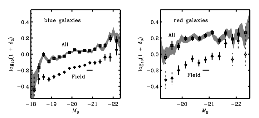
Figure 9.— (Left) We plot the logarithm of the local galaxy overdensity, $(1+\delta_{3})$, versus $B$-band absolute magnitude for all blue galaxies in Sample C. The blue population is selected according to the color division presented by Willmer et al. (2005). We measure the weighted mean dependence of environment on luminosity with the mean computed using a sliding box of width given by the black dash in the plot and weighted according to the inverse selection volumes, $1/V_{\rm max}$. The grey region corresponds to the sliding 1-$\sigma$ uncertainties in this weighted mean. The square points give the weighted mean environments and 1-$\sigma$ uncertainties in the means computed in distinct bins of $M_{B}$, thereby avoiding the covariance associated with the sliding mean. Means computed in bins containing less than 50 galaxies have been drawn with dotted error bars to signify that the uncertainty in these points has likely been underestimated. The diamond points and error bars show the weighted mean environments and 1-$\sigma$ uncertainties in the means computed in indentical luminosity bins for the field galaxy population solely. The field population is selected according to the galaxy group finder of Gerke et al. (2005), excluding all galaxies identified as group members. (Right) We make an identical plot, restricting the sample to all red galaxies drawn from Sample C according to the color division of Willmer et al. (2005). The total number of blue galaxies is 12,120, while 2,094 comprise the red galaxy sample. Similar to studies at $z\sim 0$, we find a strong trend between mean environment and luminosity for red galaxies at $z\sim 1$. However, we also observe a comparable trend with the blue galaxy population that is not found locally.

Figure 9 shows the mean dependence of galaxy overdensity on absolute $B$-band magnitude for the red and blue galaxy populations in the data sample. For the red population, we find clear evidence for luminosity dependence similar to that found locally; over the entire luminosity range probed by the survey, the mean overdensity for red galaxies increases with luminosity. Our results, however, probe a significantly smaller portion of the galaxy luminosity function than similar studies at low redshift; DEEP2 is unable to study the faintest red galaxies at high redshift which do not make the $R_{\rm AB}\leq 24.1$ magnitude limit for the survey, while the most luminous red galaxies observed in the SDSS are very rare, so few are included in the much smaller DEEP2 survey volume.

Among the blue $z\sim 1$ population, we find a clear slope in the relation between mean environment and $B$-band absolute magnitude, with brighter blue galaxies found on average in regions of greater overdensity. This trend strongly contrasts local studies by Hogg et al. (2003) and Blanton et al. (2003a), which find that the mean environment of blue galaxies is independent of luminosity. If we fit $\langle\log(1+\delta_{3})(M_{B})\rangle$ as a linear function of $M_{B}$, we find consistent slopes for the red and blue samples, with values of $-0.85\pm 0.35\log(1+\delta_{3})/M_{B}$ and $-1.26\pm 0.12\log(1+\delta_{3})/M_{B}$, respectively (see Table 2).

Restricting our sample to the field population using the group finder of Gerke et al. (2005), we find that the dependence of mean environment on $B$-band luminosity in the field shows a steeper slope $(-2.65\pm 0.47\log(1+\delta_{3})/M_{B}$ and $-1.93\pm 0.15\log(1+\delta_{3})/M_{B})$ for both the blue and red galaxy populations, respectively. Red field galaxies, however, are rare at $z\sim 1$ and thus the measured luminosity-environment trend among the red population is rather noisy. Among the blue galaxy field sample, though, the sample size is statistically significant. Within the blue field population, the mean environment is at or below the mean survey density $(\log{1+\delta_{3}}=0)$ over the entire luminosity range probed.

5.4. Predicting Environment from Galaxy Properties

Results from §5.2 indicate that galaxy color is more closely related to environment than [OII] equivalent width is at $z\sim 1$. To study this quantitatively, we compute the $1/V_{\rm max}$-weighted variance $(\sigma^{2})$ of the overdensity $(1+\delta_{3})$ measures and compare to the variance computed relative to the mean overdensity as a function of galaxy property $X$, $\sigma^{2}_{X}$, where

$$\sigma^{2}_{X}=\left\langle\left[\log(1+\delta_{3,i})-\overline{\log(1+\delta_{3})}\left(X_{i}\right)\right]^{2}\right\rangle.$$ (1)

This metric, which we use following Blanton et al. (2003a), gives the scatter about the mean relation between property $X$ and overdensity and has the benefit of being independent of the differing units for differing quantities $X$. In Table 3, we present the values of $(\sigma^{2}_{X}-\sigma^{2})$ for each property examined in this work and for each pair of properties. The $1/V_{\rm max}$-weighted variance in the measured overdensity values, $\sigma^{2}$, is 0.410 for the sample, and from the errors in the overdensity values alone, we expect a scatter of 0.249. While the local study by Blanton et al. (2003a) considered a slightly different set of galaxy properties (rest-frame color, luminosity, and morphology), our results are in agreement with their findings. For the DEEP2 sample, rest-frame $(U-B)_{0}$ color is the galaxy property most predictive of environment, among those tested. As a pair, galaxy color and luminosity show the greatest correlation with the observed galaxy densities, explaining only $\sim 10\%$ of the variation.

5.5. Environment as a Function of Color and Luminosity

As shown in §5.3, the dependence of mean environment on luminosity is very similar for both red and blue galaxy populations at $z\sim 1$. This suggests that the mean dependence of overdensity on rest-frame color and absolute magnitude may be separated into two functions:

$$\left\langle\log(1+\delta_{3})\left[M_{B},(U-B)_{0}\right]\right\rangle=f\left[\left(U-B\right)_{0}\right]+g\left[M_{B}\right]$$ (2)

where the mean dependence on galaxy color, $f[(U-B)_{0}]$, is given by the $6^{\rm th}$-degree-polynomial fit to the observed correlation with $(U-B)_{0}$ color as shown in Figure 5 and Table 2, and the mean dependence on luminosity is a linear fit derived from Figure 9 in §5.3 and listed in Table 2. In this analysis, we limit the sample to the regime $0.75<z<1.05$ where evolution in the measured density values is small and the red galaxy population is least affected by the survey target-selection.

In the top-left panel of Figure 10, we show the mean environment as a function of both color and luminosity for galaxies within $0.75<z<1.05$. The strong trend with galaxy color is evident as well as the dependence on luminosity. Using the model given in equation 2, we predict the mean dependence of environment on $(U-B)_{0}$ and $M_{B}$, as shown in the top-right panel of Figure 10. Within the errors of our measurements, the model accurately predicts the mean overdensity over the entire color-magnitude space. The bottom panels of Figure 10 show the residuals between the data and the model, which are only slightly non-Gaussian.

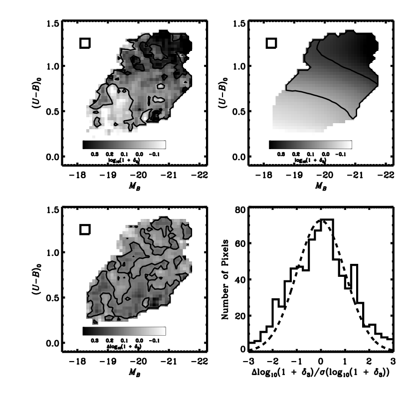
Figure 10.— (Top Left) We display the $1/V_{\rm max}$-weighted mean galaxy overdensity, $\log{(1+\delta_{3})}$, as a function of galaxy color, $(U-B)_{0}$, and absolute magnitude, $M_{B}$, computed in a sliding box of width $\Delta M_{B}=0.3$ and height $\Delta(U-B)_{0}=0.1$. The size and shape of the box are illustrated in the upper right-hand corner of the plot. Darker areas in the image correspond to regions of higher average overdensity in color-magnitude space with the scale given in the color-bar. The contours correspond to overdensity levels of $\log{(1+\delta_{3})}=0.0,0.2,0.4$. At regions where the sliding box includes less than 20 galaxies, the mean environment is not displayed. (Top Right) The mean environment as a function of color and magnitude as predicted by our separable model, $\left\langle\log(1+\delta_{3}\left(M_{B},(U-B)_{0}\right))\right\rangle=\left\langle\log(1+\delta_{3}\left(M_{B}\right))\right\rangle+\left\langle\log(1+\delta_{3}\left((U-B)_{0}\right))\right\rangle$ using the same sliding box. The overlayed contours correspond to the same mean overdensity levels as traced in the Top Left image. (Bottom Left) We display the residual mean enviroment $\log{(1+\delta_{3,{\rm data}})}-\log{(1+\delta_{3,{\rm model}})}$ as a function of color and magnitude computed in the same sliding box. The contour plotted corresponds to a residual of zero $\sigma$. (Bottom Right) We plot the distribution of residuals in units of $\sigma(<\log\delta_{3}(M_{B},(U-B)_{0})>)$ for all regions where the sliding box contains 20 or more galaxies. The distribution is roughly Gaussian with $\sim 50\%$ of the positions having a residual with absolute value greater than 1-$\sigma$. Overplotted for comparison is a Gaussian distribution of amplitude 65 pixels and dispersion of unity. The dependence of mean environment on rest-frame color and luminosity at $z\sim 1$ is well represented by a separable function of the form $\left\langle\log\delta_{3}\left(M_{B},(U-B)_{0}\right)\right\rangle=\left\langle\log\delta_{3}\left(M_{B}\right)\right\rangle+\left\langle\log\delta_{3}\left((U-B)_{0}\right)\right\rangle$.

6. Discussion

6.1. The Downsizing of Quenching

Recent studies of the galaxy luminosity function at $z\sim 1$ (e.g. Bell et al., 2004; Faber et al., 2005) indicate that the build-up of stellar mass at the high-mass end of the red sequence from $0\lesssim z\lesssim 1$ did not occur due to star formation within red galaxies. Instead, these studies conclude that massive red galaxies observed locally migrated to the bright end of the red sequence by a combination of two processes: (1) the suppression of star formation in blue galaxies (that is, the “quenching” of blue galaxies) and (2) the merging of less-luminous, previously-quenched red galaxies. With respect to the first scenario, Faber et al. (2005) discuss the growing body of evidence suggesting that the typical mass at which a blue, star-forming galaxy is quenched has decreased with time, the so-called “downsizing of quenching”. The theory of downsizing has been explored in the literature for quite some time (see e.g. Faber et al., 2005, and references therein), with Cowie et al. (1996) first presenting the concept in terms of a decline with redshift in the typical mass of star-forming galaxies. While the process of quenching and the activity of star formation are clearly closely related, the typical time-scale for each may have a different dependence on mass. Here, we will focus our discussion on the aspect of quenching within the larger picture of downsizing.

The correlations between environment and galaxy properties at $z\sim 1$, as presented in this paper, add further observational support to the proposed downsizing of quenching with redshift. In contrast to the observed $z\sim 0$ trends, we find a clear dependence of mean environment on luminosity for blue galaxies, with the brightest blue galaxies residing in regions of greater overdensity. These bright blue galaxies are also known to populate the high-mass end of the color-magnitude blue cloud, with stellar masses of $\sim{\rm a\ few}\times 10^{10}\ {\rm M}_{\sun}$ (Bundy et al., 2006; Cooper et al., 2006a) and are preferentially found in regions of high overdensity where quenching is most likely to occur, the locations in models where it is driven by galaxy mergers, the stripping of gas by hydrodynamical and tidal effects, or AGN. Furthermore, those mechanisms which can cause the total stellar mass of a large galaxy to decrease (e.g. galaxy harassment) are only effective in the most massive clusters, which are not represented within the DEEP2 sample (see §6.2). Therefore, it is extremely unlikely that these galaxies can decrease in stellar mass from $z\sim 1$ to $z\sim 0$. Thus, we conclude that the bright blue galaxies in overdense environments at high redshift evolve (i.e., have their star formation quenched) into members of the red sequence by $z\sim 0$. As such, our results within the larger set of observations suggest that the typical entry point onto the red sequence via quenching is fainter (i.e., less massive) at $z\sim 0$ than at $z\sim 1$. That is, the luminosity dependence of the mean environment for blue galaxies within the DEEP2 sample, when compared with the local SDSS and recent DEEP2 results, is consistent with a “downsizing of quenching” as discussed by Faber et al. (2005), in the sense that there exists a population of massive galaxies that was likely undergoing quenching at $z\sim 1$, which has no high-mass counterpart today. As part of an upcoming paper (Cooper et al., 2006a), we intend to examine these trends in detail by including stellar mass determinations alongside environment, color, and luminosity measures.

6.2. The Roles of Field, Group, and Cluster Environments at High Redshift

Using the group finder of Gerke et al. (2005), we can associate each galaxy in our analysis with either a cluster, a group, or the field. This provides an interesting way to examine the contribution from bound structures of different size to the environmental trends presented in §5. The DEEP2 galaxy catalog is dominated by group and field galaxies, with large clusters only scarcely represented. As illustrated in Fig. 5, the relationship between median environment and rest-frame color mirrors the dependence observed for the mean, with the median relation negligibly affected by cluster members. Within the survey volume (sample C), only $\sim 2\%$ of galaxies are found in clusters (i.e. groups with velocity dispersions greater than $500\ {\rm km}/{\rm s}$ and $N_{\rm group}>4$ observed members). For the red sequence alone, the contribution is only slightly larger at $\lesssim 3\%$. On the other hand, field galaxies represent $\sim 67\%$ of the total, with the remaining $\sim 30\%$ locked into galaxy groups. Such groups contain on average $\sim 3$ members in the survey sample, thus $\sim 5\ L_{*}$ members overall given the $\sim 60\%$ sampling rate of the DEEP2 survey.

Knowing that cluster-sized objects within the DEEP2 survey volume make a negligible contribution to our results allows us to place constraints on the physical processes which may or may not have had a role in establishing the color-environment and luminosity-environment relationships. For example, in highly overdense environments numerous mechanisms have been identified that can potentially alter the colors of the cluster population, including ram-pressure stripping (Gunn & Gott, 1972; Abadi et al., 1999), galaxy harassment (Moore et al., 1996, 1998), and global tidal interactions within the cluster potential (Byrd & Valtonen, 1990; Valluri, 1993). Although such processes all modify the star-formation histories of the galaxies on which they operate, such environments are not present in the DEEP2 sample in any statistically significant sense and the aforementioned processes do not operate efficiently in lower-density environments such as groups. Thus, these cluster-specific mechanisms alone cannot explain the established environmental relationships observed at $z\sim 1$.

The interesting flip-side to the above discussion is that both group-sized systems and galaxies in the field are abundant in the DEEP2 galaxy catalog. Such sub-populations offer an alternative place to look to understand the observed color- and luminosity-environment trends. To disentangle the contribution from each, we first remove all group and cluster members from the sample and then recompute each of our main results. In Figure 5, we overplot the $z\sim 1$ relation between mean overdensity and galaxy rest-frame $(U-B)_{0}$ color for field galaxies alone (diamond symbols). We find that for the field population only a weak trend of overdensity with galaxy color persists, where red field galaxies are found to be only marginally overdense relative to their blue counterparts. Thus, not surprisingly, group-sized systems play a dominant role in establishing the density contrast observed at the color bimodality within the color-environment relation at $z\sim 1$.

While the difference in mean overdensity between red and blue galaxies is reduced by excluding group members, the trend towards lower mean overdensity at very blue colors is barely altered. The preservation of this trend among the field population is not surprising given the small fraction $(\sim 20\%)$ of galaxies at the bluest colors $((U-B)_{0}<0.3)$ that are in groups. Based on their [OII] equivalent widths, these very blue galaxies have the highest specific star-formation rates within the DEEP2 sample, which indicates that their stellar populations are predominantly composed of young stars. The nature of this interesting subpopulation will be investigated more throughly by Croton et al. (2006).

Having isolated the DEEP2 field galaxy population, we examine the dependence of overdensity on rest-frame $B$-band absolute magnitude for blue-cloud and red-sequence galaxies separately, as shown in Figure 9 (diamond symbols, top and bottom panels, respectively). Red-sequence field galaxies show a decrease in density contrast relative to the full red sequence across the entire magnitude range probed. Unfortunately, as such galaxies are rather rare within the DEEP2 sample, the statistics we obtain are somewhat noisy. Blue field galaxies, on the other hand, are greater in number within DEEP2 and exhibit an interesting relationship between environment and luminosity; when the contribution from group galaxies is removed, their contrast in density also decreases. However, the slope of this trend from faint to bright appears to have steepened somewhat (see Fig. 9 and Table 2), with the faintest blue field galaxies characteristically populating survey regions with overdensities approaching those of voids and the brightest blue field galaxies residing on average in environments of mean survey density $(\log{\delta_{3}}=0)$.

This behavior is consistent with current observations of the local galaxy population, where the characteristic luminosity of the blue field population also scales with environment, at least in under- to mean-density regions of the universe (see Figure 7 of Croton et al., 2005b). Thus in comparison to the results of Croton et al. (2005b), at least qualitatively, the blue sequence field population shows a similar relationship with environment at both $z\sim 1$ and the present day. This contrasts the bright blue group members, which through the quenching of their star formation must transition onto the red sequence where they are observed today in the local universe. This leads us to propose that at $z\gtrsim 1$ quenching is a process that dominates galaxy evolution down to systems of group size and not below. Note that, although some red galaxies are found to reside in low density environments at $z\sim 1$ they constitute only a small portion of the field population ($\lesssim 15\%$ Gerke et al., 2006). Conceivably, some of these galaxies could belong to groups missed by our group finder or to fossil groups of high virial mass but with underluminous satellite members. A more thorough study of the relationship between environment and luminosity in group and field galaxies in the SDSS or the 2dFGRS is truly needed to measure the luminosity-environment trend among the blue field population locally, thereby completing this picture.

6.3. The Physics of Quenching

One may naturally ask exactly what physical processes could have occurred within both cluster and group environments to explain the observed color and magnitude relations with respect to overdensity presented in this paper. We have already pointed out that many mechanisms that dominate cluster-sized systems alone are unlikely to explain our results, as they do not operate efficiently in the lower-mass halos where our results show they need to. We will now discuss several processes that may be operating in this lower-mass regime.

As shown by Birnboim & Dekel (2003), Kereš et al. (2005), and Croton et al. (2005a), models of gas infall onto dark matter halos produce a natural bimodal distribution in gas temperature, dividing cold infalling gas from that which remains at the virial temperature to form a static hot halo. The dominant component of gas in a system, cold or hot, is found to change at a reasonably well defined dark matter halo mass of approximately $2-3\times 10^{11}\ {\rm M}_{\sun}$ out to at least $z\sim 6$. Interestingly, this mass is low enough to include systems which are identified observationally as groups; within the DEEP2 survey, galaxy groups are found to occupy dark matter halos with masses both above and below this critical mass (Coil et al., 2005). The above authors speculate that as a growing dark matter halo passes this critical mass, the infalling cold gas supply to the central galactic disk is shut off, and the galaxy will quickly burn its remaining fuel and redden (see also Dekel & Birnboim, 2005). Within this picture, blue galaxies in the DEEP2 $z\sim 1$ sample are only just approaching this critical halo mass and will still be cold-accreting infalling gas from which star formation is fueled, even for the brightest blue galaxies in the densest environments (Figure 9). However, dark matter halos continue to grow at redshifts of $z<1$, and thus these systems may eventually reach the transition mass, at which point the infalling gas instead heats to the virial temperature to build a quasistatic hot halo around the galaxy. If there is no subsequent cold gas supply to the disk, then star formation in such galaxies will ultimately become quenched, as observed in the local universe.

The primary problem with this picture is that in systems more massive than the critical halo mass, quasistatic x-ray emitting hot atmospheres typically have central cooling times much shorter than the age of the universe (e.g. Fabian, 2003). The hot, dense central regions must then cool, and the gas condensing out of the flow will ultimately reach the galactic disk to feed the central galaxy star-formation reservoir, in a similar way as the infalling cold-accreting gas would when the system was much less massive. This is the classical “cooling flow problem” and has been extensively investigated in the literature over the past 30 or so years (see e.g. Fabian, 1994; McNamara, 2002). If left unabated, such unconstrained star formation can keep even the most massive galaxy in the “blue cloud” (Croton et al., 2005a), in stark contrast to what is observed. Because of this, the transition from cold to hot accretion for a galaxy halo is unlikely to be able to account for the observed quenching of $z\sim 1$ bright blue galaxies alone. Many authors have thus proposed AGN as an energetically feasible mechanism with which cooling gas can be suppressed (e.g. Binney, 2001; Zanni et al., 2005; Sanderson et al., 2005, and references therin). Croton et al. (2005a) demonstrate that if one assumes a low energy AGN heating source fed from the quiescent hot halo surrounding the galaxy (which, from above, can form when the host dark matter halo reaches a mass of $\sim 10^{11}{\rm M}_{\sun}$), then the cooling flow gas can be effectively stopped, thereby quenching star formation and pushing the galaxy from the blue cloud and onto the red sequence.

Other group-scale processes may also contribute to the quenching of star formation. In addition to the mechanisms just discussed, galaxy mergers, which preferentially occur in galaxy groups (Cavaliere et al., 1992; Navarro et al., 1987), may be capable of triggering events which remove cold gas from the galactic disk to shut off star formation, at least for some (perhaps extended) period of time. Such events can then potentially convert members of the blue cloud into red-sequence galaxies. Early simulation work showed that mergers can disrupt galactic disks yielding merger remnants with surface-brightness profiles and density distributions similar to those of elliptical galaxies (Toomre & Toomre, 1972; Barnes, 1989; Barnes & Hernquist, 1992). Along with a morphological transformation, merger events in systems rich in cold gas can also produce starbursts from which strong galactic super-winds flow (Cox et al., 2005; Benson et al., 2003), and merger-induced cold gas accretion on to central super-massive black holes can trigger energetic quasar winds which are capable of sweeping all gas from their hosts (Murray et al., 2005; Hopkins et al., 2005; Robertson et al., 2005; Di Matteo et al., 2005). In this way, a merger may initiate additional processes which result in a depletion of the star forming gas reservoir, leading ultimately to a quenching of the galaxies star formation if no addition cold gas supply is present.

We conclude this section by mentioning an additional process that may be relevant to the present discussion, but may not be described as an environment-dependent effect. Secular evolution (or secular bulge-building) is another means of triggering morphological evolution in a galaxy (e.g. Zhang, 1996; Kormendy & Kennicutt, 2004; Kormendy & Fisher, 2005, and references therein). Following secular evolution, subcomponents of a galaxy interact internally through the transfer of angular momentum along a galactic bar (or spiral arms), from which matter can funnel inwards towards the galactic center. For example, Noguchi (1999) suggests that the bulges of disk galaxies may result from the accumulation of massive clumps that formed within the galactic disk and migrated inward via dynamical friction. Such instabilities provide a channel through which cold gas in the disk can transfer away its angular momentum to reach the central regions of the galaxy, potentially providing a source of fuel to the central black hole to trigger an AGN outflow, as described above. The results presented within this paper, however, suggest that the quenching of blue galaxies is an evolutionary process that occurs preferentially in overdense environments. Thus, it appears as if secular evolution cannot be the only process responsible for the trends with environment observed at $z\sim 1$.

6.4. Evolution of Environment Trends from $z\sim 1$ to $z\sim 0$

While a clear relationship between rest-frame color and environment is already in place by a redshift of unity, and comparison to local samples indicates that star formation is being suppressed in more massive galaxies at $z\sim 1$ than at $z\sim 0$, we are unfortunately not yet able to precisely quantify the differences between the two populations or the strength of this evolution. Such a quantitative analysis requires establishing the local and $z\sim 1$ galaxy samples on equal footing, for example, by measuring galaxy colors and luminosities in identical passbands and measuring environments using identical techniques and with equivalent galaxy samples. While beyond the scope of this current paper, future work utilizing the DEEP2 and SDSS data sets (Cooper et al., 2006c) will address this issue.

It is possible, however, to combine the environment measurements at $z\sim 1$ and $z\sim 0$ into a general picture of how the overall galaxy population evolves. Here, we discuss the results presented in this work and similar low-$z$ studies (e.g., Hogg et al., 2003; Blanton et al., 2003a), in light of both the larger framework of clustering evolution and the need for quenching mechanisms that operate most efficiently in group- and cluster-sized systems. The color-environment relations at low- and high-redshift epochs show amazing similarity in general. While quantifying the evolution in this relationship will be addressed in another paper, we speculate that the contrast in mean overdensity between red and blue galaxies increases from $z\sim 1$ to $z\sim 0$ as blue galaxies in overdense environments are preferentially quenched and join the red sequence and as already-quenched red galaxies continue to cluster into increasingly overdense environments.

This larger picture is also consistent with the observed trends between environment and luminosity for both red and blue galaxy populations. Unlike similar $z\sim 0$ studies, the DEEP2 survey unfortunately does not sample the faint end of the red galaxy luminosity function due to the $R_{AB}$ magnitude limit of the survey. At bright magnitudes, however, we find a trend towards increasing mean environment with luminosity for red galaxies similar to that found locally. The increasingly steep slope to the $z\sim 0$ luminosity-environment relation at the very bright end of the red sequence (Hogg et al., 2003; Blanton et al., 2003a) is not seen in our higher-redshift results. To build such bright red massive galaxies requires cluster environments, which are relatively rare at $z\sim 1$ but increase in number in a highly-evolved clustering distribution as seen locally.

For blue galaxies in all environments, the $z\sim 1$ relationship between mean overdensity and luminosity is significantly different from that seen at $z\sim 0$, with a strong slope such that bright blue galaxies are preferentially found in regions of higher overdensity and faint blue galaxies in underdense regions. In contrast, Croton et al. (2005a), suggest that the blue field galaxy population at low redshift shows a luminosity-environment trend quite similar to the $z\sim 1$ relation presented in this paper. Evolution such as this could be expected, if as the clustering of the galaxy distribution evolves, the bright blue galaxies in overdense regions at $z\sim 1$ are preferentially quenched, while the faint blue cluster population becomes increasingly numerous from satellites first falling into denser regions. This evolution at the bright and faint end of the blue population would cause the trend between environment and luminosity along the blue cloud to flatten, thereby explaining the $z\sim 0$ results of Hogg et al. (2003) and Blanton et al. (2003a).

In future work, we will attempt to clarify the exact physical processes responsible for the quenching of blue, star-forming galaxies by studying the relationship between environment, AGN activity, and galaxy morphology within the DEEP2 data set (Cooper et al., 2006a). There the multiwavelength data of the Extended Groth Strip (EGS) will be invaluable in identifying the AGN population, and high-resolution HST/ACS imaging will be critical for classifying galaxy morphologies.

7. Conclusions

In this paper, we present the first study of the relationships between galaxy properties and environment at $z\sim 1$ to cover a broad and continuous range of environment from groups to weakly-clustered field galaxies. Using a sample of galaxies drawn from the DEEP2 Galaxy Redshift Survey, we estimated the local overdensity about each galaxy according to the projected $3^{\rm rd}$-nearest-neighbor surface density. We study the relationships between environment and galaxy color, luminosity, and [OII] equivalent width. Our principal results are:

1. We find a strong dependence of mean environment on rest-frame $(U-B)_{0}$ color (Fig. 5), with blue galaxies on average occupying regions of lower density than red galaxies. The observed trend with galaxy color echoes the results of studies of nearby galaxies (e.g. Hogg et al., 2003; Blanton et al., 2004); all features of the global correlation between galaxy color and environment measured at $z\sim 0$ are found to be already in place at $z\sim 1$.

2. For the red galaxy population at $z\sim 1$, we see clear evidence for a dependence of mean overdensity on luminosity, mirroring results from local studies (Fig. 9). Unlike the SDSS, however, DEEP2 does not probe the faint red galaxy population and includes relatively few luminous red galaxies due to the smaller survey volume, rendering the strongest effects seen locally undetectable.

3. While low redshift studies find the mean environment of blue galaxies to be independent of luminosity, we find a strong increase in local density with luminosity for blue galaxies at $z\sim 1$ (Fig. 9). Restricting to the blue field population in the DEEP2 survey, the dependence of mean overdensity on $B$-band luminosity persists, with the mean environment at or below the mean survey density over the luminosity range probed.

4. The pair of galaxy properties which best predict environment at $z\sim 1$ are galaxy color and luminosity (Table 3). Additionally, while we do measure a modest difference in luminosity dependence for the mean environments of blue and red galaxies, we show that the dependence of environment on $M_{B}$ and $(U-B)_{0}$ is well represented by a separable function (Fig. 10).

5. The mechanisms of ram-pressure stripping, galaxy harassment, and global tidal interactions, which preferentially occur in clusters, cannot alone explain the observed relationships between galaxy properties and environment at $z\sim 1$.

6. Our results are consistent with a downsizing of the characteristic mass or luminosity at which the quenching of a galaxy’s star formation becomes efficient. We discuss how quenching appears to be a process that must operate efficiently in both cluster and group environments for consistency between our results and those at redshift $z\sim 0$. AGN heating of cooling gas may satisfy this requirement, however the exact quenching mechanism still remains an open question.

Table 1 Galaxy Samples

Sample	Redshift Range	Edge Distance	$W_{\rm[OII]}$	# of Galaxies
Sample A	$0<z<2$	$\cdots$	$\cdots$	23,004
Sample B	$0.75<z<1.35$	$\cdots$	$\cdots$	18,977
Sample C	$0.75<z<1.35$	$>1h^{-1}\ {\rm Mpc}$	$\cdots$	14,214
Sample D	$0.75<z<1.35$	$>1h^{-1}\ {\rm Mpc}$	$\sigma_{W_{\rm[OII]}}<10$Å	11,250
Sample E	$0.75<z<1.05$	$>1h^{-1}\ {\rm Mpc}$	$\cdots$	9,567

Note. — We list all of the galaxy samples used in this work. For each sample, we give the redshift range over which galaxies are selected, any restrictions applied regarding the distance to the nearest survey edge (see §4.2) or according to error in equivalent width (see §3.2). In the final column, we detail the number of galaxies included in each sample. All samples are restricted to sources with accurate redshift determinations (Q=3 or Q=4 redshifts as defined by Faber et al. (2006)).

Table 2 Polynomail Fits to Mean Relations

	$a_{0}$	$a_{1}$	$a_{2}$	$a_{3}$	$a_{4}$	$a_{5}$
$(U-B)_{0}$	-0.658	4.865	-15.126	21.662	-13.762	3.175
$M_{B}[{\rm blue}]$	-1.249	-0.063	$\cdots$	$\cdots$	$\cdots$	$\cdots$
$M_{B}[{\rm red}]$	-0.826	-0.049	$\cdots$	$\cdots$	$\cdots$	$\cdots$

Note. — We list the coefficients for the polynomial fit to the mean environment versus color relation (see Fig. 5. Also listed are the coefficients for the linear fits to the mean environment versus absolute magnitude relations for red and blue galaxies (see Fig. 9). For each, the functional form of the fit is given by $f(x)=a_{0}+a_{1}x+a_{2}x^{2}+\cdots$.

Table 3 Correlation of Properties and Environment

Galaxy Property	$(\sigma^{2}_{X}-\sigma^{2})$	$(U-B)_{0}$	$W_{\rm[OII]}$	$M_{B}$
$(U-B)_{0}$	-0.0076	$\cdots$	-0.0075	-0.0160
$W_{\rm[OII]}$	-0.0019	-0.0075	$\cdots$	-0.0147
$M_{B}$	-0.0031	-0.0160	-0.0147	$\cdots$

Note. — For each galaxy property studied in this paper, the second column gives the values of $\sigma^{2}_{X}-\sigma^{2}$. The entries in the right three columns give the difference in variance, $\sigma^{2}_{X,Y}-\sigma^{2}$, where $\sigma^{2}_{X,Y}$ is the variance about the mean relations for the pair of properties $X$ and $Y$. In this table, lower values indicate that the galaxy property or pair of properties are a better predictor of environment. Rest-frame color, $(U-B)_{0}$, is the single best predictor of environment among the properties studied, while the combination of color and $B$-band luminosity are the most strongly correlated pair of properties with environment, on average.

References

- Abadi et al. (1999) Abadi, M. G., Moore, B., & Bower, R. G. 1999, MNRAS, 308, 947
- Baldry et al. (2004) Baldry, I. K., Glazebrook, K., Brinkmann, J., Ivezić, Ž., Lupton, R. H., Nichol, R. C., & Szalay, A. S. 2004, ApJ, 600, 681
- Balogh et al. (2004a) Balogh, M. et al. 2004a, MNRAS, 348, 1355
- Balogh et al. (2004b) Balogh, M. L., Baldry, I. K., Nichol, R., Miller, C., Bower, R., & Glazebrook, K. 2004b, ApJ, in press [astro–ph/0406266]
- Balogh et al. (1998) Balogh, M. L., Schade, D., Morris, S. L., Yee, H. K. C., Carlberg, R. G., & Ellingson, E. 1998, ApJ, 504, L75+
- Barnes (1989) Barnes, J. E. 1989, Nature, 338, 123
- Barnes & Hernquist (1992) Barnes, J. E. & Hernquist, L. 1992, ARA&A, 30, 705
- Beers et al. (1990) Beers, T. C., Flynn, K., & Gebhardt, K. 1990, AJ, 100, 32
- Bell et al. (2004) Bell, E. F., Wolf, C., Meisenheimer, K., Rix, H., Borch, A., Dye, S., Kleinheinrich, M., Wisotzki, L., & McIntosh, D. H. 2004, ApJ, 608, 752
- Benson et al. (2003) Benson, A. J., Bower, R. G., Frenk, C. S., Lacey, C. G., Baugh, C. M., & Cole, S. 2003, ApJ, 599, 38
- Bessell (1990) Bessell, M. S. 1990, PASP, 102, 1181
- Binney (2001) Binney, J. 2001, in ASP Conf. Ser. 250: Particles and Fields in Radio Galaxies Conference, 481–+
- Birnboim & Dekel (2003) Birnboim, Y. & Dekel, A. 2003, MNRAS, 345, 349
- Blanton et al. (2003a) Blanton, M. R., Eisenstein, D. J., Hogg, D. W., Schlegel, D. J., & Brinkmann, J. 2003a, ApJ, submitted [astro–ph/0310453]
- Blanton et al. (2004) Blanton, M. R., Eisenstein, D. J., Hogg, D. W., & Zehavi, I. 2004, ApJ, submitted [astro–ph/0411037]
- Blanton et al. (2003b) Blanton, M. R. et al. 2003b, ApJ, 594, 186
- Bundy et al. (2006) Bundy, K. et al. 2006, ApJ, in preparation
- Burles & Schlegel (2006) Burles, S. & Schlegel, D. J. 2006, in preparation
- Byrd & Valtonen (1990) Byrd, G. & Valtonen, M. 1990, ApJ, 350, 89
- Cavaliere et al. (1992) Cavaliere, A., Colafrancesco, S., & Menci, N. 1992, ApJ, 392, 41
- Christlein & Zabludoff (2005) Christlein, D. & Zabludoff, A. I. 2005, ApJ, 621, 201
- Coil et al. (2004a) Coil, A. L., Newman, J. A., Kaiser, N., Davis, M., Ma, C., Kocevski, D. D., & Koo, D. C. 2004a, ApJ, 617, 765
- Coil et al. (2004b) Coil, A. L. et al. 2004b, ApJ, 609, 525
- Coil et al. (2005) —. 2005, ApJ, accepted [astro-ph/0507647]
- Cole et al. (2000) Cole, S., Lacey, C. G., Baugh, C. M., & Frenk, C. S. 2000, MNRAS, 319, 168
- Colless et al. (2001) Colless, M. et al. 2001, MNRAS, 328, 1039
- Cooper et al. (2005) Cooper, M. C., Newman, J. A., Madgwick, D. S., Gerke, B. F., Yan, R., & Davis, M. 2005, ApJ, 634, 833
- Cooper et al. (2006a) Cooper, M. C. et al. 2006a, MNRAS, in preparation
- Cooper et al. (2006b) —. 2006b, ApJ, in preparation
- Cooper et al. (2006c) —. 2006c, MNRAS, in preparation
- Couch et al. (1998) Couch, W. J., Barger, A. J., Smail, I., Ellis, R. S., & Sharples, R. M. 1998, ApJ, 497, 188
- Cowie et al. (1996) Cowie, L. L., Songaila, A., Hu, E. M., & Cohen, J. G. 1996, AJ, 112, 839
- Cox et al. (2005) Cox, T. J., Di Matteo, T., Hernquist, L., Hopkins, P. F., Robertson, B., & Springel, V. 2005, ApJ, submitted [astro-ph/0504156]
- Croton et al. (2005a) Croton, D. et al. 2005a, MNRAS, submitted [astro-ph/0508046]
- Croton et al. (2006) —. 2006, MNRAS, in preparation
- Croton et al. (2005b) Croton, D. J. et al. 2005b, MNRAS, 356, 1155
- Davis & Geller (1976) Davis, M. & Geller, M. J. 1976, ApJ, 208, 13
- Davis et al. (2003) Davis, M. et al. 2003, in Discoveries and Research Prospects from 6- to 10-Meter-Class Telescopes II. Edited by Guhathakurta, Puragra. Proceedings of the SPIE, Volume 4834, pp. 161-172 (2003)., 161–172
- Davis et al. (2004) Davis, M. et al. 2004, in ”Observing Dark Energy”, Sidney Wolff and Tod Lauer, editors, ASP Conference Series, [astro–ph/0408344]
- De Lucia et al. (2005) De Lucia, G., Springel, V., White, S. D. M., Croton, D., & Kauffmann, G. 2005, [astro-ph/0509725]
- Dekel & Birnboim (2005) Dekel, A. & Birnboim, Y. 2005, [astro-ph/0412300]
- Di Matteo et al. (2005) Di Matteo, T., Springel, V., & Hernquist, L. 2005, Nature, 433, 604
- Dressler (1980) Dressler, A. 1980, ApJ, 236, 351
- Faber et al. (2003) Faber, S. M. et al. 2003, in Instrument Design and Performance for Optical/Infrared Ground-based Telescopes. Edited by Iye, Masanori; Moorwood, Alan F. M. Proceedings of the SPIE, Volume 4841, pp. 1657-1669 (2003)., 1657–1669
- Faber et al. (2005) Faber, S. M. et al. 2005, ApJ, submitted [astro-ph/0506044]
- Faber et al. (2006) —. 2006, ApJ, in preparation
- Fabian (1994) Fabian, A. C. 1994, ARA&A, 32, 277
- Fabian (2003) Fabian, A. C. 2003, in Revista Mexicana de Astronomia y Astrofisica Conference Series, 303–313
- Gómez et al. (2003) Gómez, P. L. et al. 2003, ApJ, 584, 210
- Gerke et al. (2005) Gerke, B. F. et al. 2005, ApJ, 625, 6
- Gerke et al. (2006) —. 2006, MNRAS, in preparation
- Gunn & Gott (1972) Gunn, J. E. & Gott, J. R. I. 1972, ApJ, 176, 1
- Hogg et al. (2002) Hogg, D. W., Baldry, I. K., Blanton, M. R., & Eisenstein, D. J. 2002, [astro–ph/0210394]
- Hogg et al. (2004) Hogg, D. W., Blanton, M. R., Brinchmann, J., Eisenstein, D. J., Schlegel, D. J., Gunn, J. E., McKay, T. A., Rix, H., Bahcall, N. A., Brinkmann, J., & Meiksin, A. 2004, ApJ, 601, L29
- Hogg et al. (2003) Hogg, D. W. et al. 2003, ApJ, 585, L5
- Hopkins et al. (2005) Hopkins, P. F., Hernquist, L., Cox, T. J., Di Matteo, T., Robertson, B., & Springel, V. 2005, ApJ, submitted [astro-ph/0506398
- Kauffmann et al. (1993) Kauffmann, G., White, S. D. M., & Guiderdoni, B. 1993, MNRAS, 264, 201
- Kauffmann et al. (2004) Kauffmann, G., White, S. D. M., Heckman, T. M., Ménard, B., Brinchmann, J., Charlot, S., Tremonti, C., & Brinkmann, J. 2004, MNRAS, 353, 713
- Kereš et al. (2005) Kereš, D., Katz, N., Weinberg, D. H., & Davé, R. 2005, MNRAS, 363, 2
- Kinney et al. (1996) Kinney, A. L., Calzetti, D., Bohlin, R. C., McQuade, K., Storchi-Bergmann, T., & Schmitt, H. R. 1996, ApJ, 467, 38
- Kormendy & Fisher (2005) Kormendy, J. & Fisher, D. B. 2005, in Revista Mexicana de Astronomia y Astrofisica Conference Series, 101–108
- Kormendy & Kennicutt (2004) Kormendy, J. & Kennicutt, R. C. 2004, ARA&A, 42, 603
- Lewis et al. (2002) Lewis, I. et al. 2002, MNRAS, 334, 673
- Madgwick et al. (2003) Madgwick, D. S. et al. 2003, MNRAS, 344, 847
- Malmquist (1936) Malmquist, K. G. 1936, Stockholms Observatoriums Annaler, 26
- McNamara (2002) McNamara, B. R. 2002, in ASP Conf. Ser. 262: The High Energy Universe at Sharp Focus: Chandra Science, 351–+
- Moore et al. (1996) Moore, B., Katz, N., Lake, G., Dressler, A., & Oemler, A. 1996, Nature, 379, 613
- Moore et al. (1998) Moore, B., Lake, G., & Katz, N. 1998, ApJ, 495, 139
- Murray et al. (2005) Murray, N., Quataert, E., & Thompson, T. A. 2005, ApJ, 618, 569
- Navarro et al. (1987) Navarro, J. F., Mosconi, M. B., & Lambas, D. G. 1987, MNRAS, 228, 501
- Noguchi (1999) Noguchi, M. 1999, ApJ, 514, 77
- Norberg et al. (2002) Norberg, P. et al. 2002, MNRAS, 332, 827
- Oke & Gunn (1983) Oke, J. B. & Gunn, J. E. 1983, ApJ, 266, 713
- Poggianti et al. (2005) Poggianti, B. M. et al. 2005, ApJ, submitted [astro-ph/0512391]
- Postman & Geller (1984) Postman, M. & Geller, M. J. 1984, ApJ, 281, 95
- Press et al. (1992) Press, W. H., Teukolsky, S. A., Vetterling, W. T., & Flannery, B. P. 1992, Numerical recipes in FORTRAN. The art of scientific computing (Cambridge: University Press, —c1992, 2nd ed.)
- Robertson et al. (2005) Robertson, B., Cox, T. J., Hernquist, L., Franx, M., Hopkins, P. F., Martini, P., & Springel, V. 2005, ApJ, submitted [astro–ph/0511053]
- Sanderson et al. (2005) Sanderson, A. J. R., Finoguenov, A., & Mohr, J. J. 2005, ApJ, 630, 191
- Smith et al. (2005) Smith, G. P., Treu, T., Ellis, R. S., Moran, S. M., & Dressler, A. 2005, ApJ, 620, 78
- Somerville & Primack (1999) Somerville, R. S. & Primack, J. R. 1999, MNRAS, 310, 1087
- Springel et al. (2005) Springel, V., Di Matteo, T., & Hernquist, L. 2005, ApJ, 620, L79
- Strateva et al. (2001) Strateva, I. et al. 2001, AJ, 122, 1861
- Tanaka et al. (2005) Tanaka, M., Kodama, T., Arimoto, N., Okamura, S., Umetsu, K., Shimasaku, K., Tanaka, I., & Yamada, T. 2005, MNRAS, 362, 268
- Toomre & Toomre (1972) Toomre, A. & Toomre, J. 1972, ApJ, 178, 623
- Treu et al. (2003) Treu, T., Ellis, R. S., Kneib, J.-P., Dressler, A., Smail, I., Czoske, O., Oemler, A., & Natarajan, P. 2003, ApJ, 591, 53
- Valluri (1993) Valluri, M. 1993, ApJ, 408, 57
- Weiner et al. (2005) Weiner, B. J., Phillips, A. C., Faber, S. M., Willmer, C. N. A., Vogt, N. P., Simard, L., Gebhardt, K., Im, M., Koo, D. C., Sarajedini, V. L., Wu, K. L., Forbes, D. A., Gronwall, C., Groth, E. J., Illingworth, G. D., Kron, R. G., Rhodes, J., Szalay, A. S., & Takamiya, M. 2005, ApJ, 620, 595
- Willmer et al. (2005) Willmer, C. N. A. et al. 2005, ApJ, accepted [astro-ph/0506041]
- Yan et al. (2004) Yan, R., White, M., & Coil, A. L. 2004, ApJ, 607, 739
- Yan et al. (2005) Yan, R. et al. 2005, MNRAS, in preparation
- York et al. (2000) York, D. G. et al. 2000, AJ, 120, 1579
- Zanni et al. (2005) Zanni, C., Murante, G., Bodo, G., Massaglia, S., Rossi, P., & Ferrari, A. 2005, A&A, 429, 399
- Zehavi et al. (2002) Zehavi, I. et al. 2002, ApJ, 571, 172
- Zhang (1996) Zhang, X. 1996, ApJ, 457, 125