Blind component separation for polarized observations of the CMB

Abstract

We present in this paper the PolEMICA (Polarized Expectation-Maximization Independent Component Analysis) algorithm which is an extension to polarization of the SMICA (Spectral Matching Independent Component Analysis) temperature multi-detectors multi-components (MD-MC) component separation method Delabrouille et al. 2003 . This algorithm allows us to estimate blindly in harmonic space multiple physical components from multi-detectors polarized sky maps. Assuming a linear noisy mixture of components we are able to reconstruct jointly the anisotropies electromagnetic spectra of the components for each mode $T$, $E$ and $B$, as well as the temperature and polarization spatial power spectra, $TT$, $EE$, $BB$, $TE$, $TB$ and $EB$ for each of the physical components and for the noise on each of the detectors. PolEMICA is specially developed to estimate the CMB temperature and polarization power spectra from sky observations including both CMB and foreground emissions. This has been tested intensively using as a first approach full sky simulations of the Planck satellite polarized channels for a 14-months nominal mission assuming a simplified linear sky model including CMB, and optionally Galactic synchrotron emission and a Gaussian dust emission. Finally, we have applied our algorithm to more realistic Planck full sky simulations, including synchrotron, realistic dust and free-free emissions.

1 Introduction

Mapping the Cosmic Microwave Background (CMB) polarization is one of the major challenges of future missions of observational cosmology. CMB polarization is linear and therefore can be described by the first three Stokes parameters I, Q and U which are generally combined to produce three fields (modes), $T$, $E$ and $B$ Zaldarriaga & Seljak 1997 . The polarization of the CMB photons carries extra physical informations that are not accessible by the study of the temperature anisotropies. Therefore its measurement helps breaking down the degeneracies on cosmological parameters as encounter with temperature anisotropies measurements only Zaldarriaga et al. (1997). Furthermore, the study of the CMB polarization is also a fundamental tool to estimate the energy scale of inflation which has been proposed to solve the problems of flatness, of isotropy and of the seed perturbations for the formation of the structures in the Universe. Inflationary models predict the presence of tensor perturbations of the metric which will lead to an unique signature in the CMB polarization $B$ modes. The detection of the latter would be a strong proof of such an epoch and also a way to constrain the energy scale at which inflation occurs by measuring the tensor to scalar ratio, $r$ Turner & White 1996 .

Since the beginning of the CMB anisotropies observations with the COsmic Background Explorer (COBE) Smoot et al. (1992), a great amount of experiments have been designed to determine the CMB temperature angular power spectrum Netterfield et al. (1997); Miller et al. 1999 ; deBernardis et al. 2000 ; Hanany et al. 2000 ; Lee et al. 2001 ; Netterfield et al. (2002); Halverson et al. 2002 ; Sievers et al. 2003 ; Rubino-Martin et al. 2003 ; Benoît et al. 2003 ; Hinshaw et al. 2006 ; Barkats et al. 2005 ; Readhead et al. 2004 ; Leitch et al. 2005 ; Tristram et al. (2005); Jones et al. 2005 . By contrast, the polarization anisotropies, which are between 2 and 5 orders of magnitude weaker than temperature ones are not accurately measured yet. A first detection of the CMB $E$ modes has been performed by DASI Kovac et al. (2002); Leitch et al. 2005 , CAPMAP Barkats et al. 2005 , CBI Readhead et al. 2004 and more recently by BOOMERanG Montroy et al. (2005) and WMAP Page et al. (2006). The $TE$ temperature-polarization cross correlation has been measured by WMAP Page et al. (2006) and BOOMERanG Piacentini et al. (2005). No detection of the CMB $B$ modes has been reported yet. Nevertheless, constraints on the tensor to scalar ratio, $r$, have been set by the WMAP team. They set an upper limit of $r<0.55$ (95% CL) Spergel et al. (2006) for the temperature and polarization analysis and of $r<2.2$ (95$\%$ CL) Page et al. (2006) for a polarization-only analysis.

The detection of such low signals is possible by improving the instrumental sensitivity, but this is not the only issue in the determination of the CMB polarization power spectra. Other astrophysical emissions as for example the diffuse Galactic emission including free-free, dust and synchrotron and the extragalactic-sources emissions also contribute to the sky brightness at the frequencies of interest for CMB studies, and therefore must be efficiently subtracted. These foregrounds are particularly important for the study of the CMB polarization. Excluding the free-free emission which is not polarized, the other contributions are expected to be significantly polarized with similar power on the $E$ and $B$ modes. Recent measurements of the Galactic synchrotron polarization emission at 1.41 GHz Wolleben et al. 2005 and at 23 GHz by WMAP Page et al. (2006) show this emission is significantly polarized at large angular scales. Further, Archeops measurements at 353 GHz show that the Galactic dust diffuse emission is polarized up to a level of 5 to 10 % both in the Galactic center Benoît et al. 2004 and at high Galactic latitudes Ponthieu et al. (2005). Finally, for the polarization of extragalactic point sources the sparsity of the data available makes reliable predictions difficult Tucci et al. 2004 ; Hildebrand (1996).

A direct subtraction of these foreground contributions on the CMB data will require an accurate knowledge of their spatial distributions and of the electromagnetic spectra of their anisotropies. For the synchrotron emission a full sky map at 408 MHz in temperature is available Haslam et al. (1982) and more recently the WMAP team provided a map at 30 GHz from the MEM decomposition of the first year observations Bennett et al. 2003b . A fake polarized synchrotron emission template was constructed by Giardino et al. (2002) based on the Parkes 2400 MHz Duncan et al. 1997 and Haslam 408 MHz Haslam et al. (1982) surveys. Furthermore, the electromagnetic spectrum of synchrotron anisotropies and its spatial distribution are neither accurately known in temperature nor polarization although a first estimate was produced by Giardino et al. (2002). Recently, the 23 GHz polarized WMAP data is used as a tracer of the synchrotron polarization Page et al. (2006). For the thermal dust emission a full sky map at 100 $\mu$m as well as templates for CMB use were extracted from the IRAS and FIRAS data Schlegel et al. (1998); Finkbeiner et al. 1999 . No realistic template exists for the dust polarized emission, although a fake one, based on the polarization angles measured at 23 GHz has been constructed by the Planck collaboration. The dust emission in temperature can be approximated by a grey body spectrum of mean temperature 17 K and emissivity between 1.7 and 2.2 Finkbeiner et al. 1999 ; Lagache et al. 2003 . Currently no measurement on the electromagnetic spectrum of the dust polarized emission is available although it is expected to be the same that for temperature Jones et al. 1992 .

To try to overcome the above limitations, a great amount of work has been dedicated to design and implement algorithms for component separation which can discriminate between CMB and foregrounds. These methods can also extract, directly from the CMB data, the emission properties of foregrounds. Wiener filtering has been successfully tested assuming known Gaussian priors for each component and with the electromagnetic spectrum of the anisotropies as an input Tegmark & Efstathiou (1996); Bouchet et al. 1999 . Maximum entropy based methods (MEM), assuming entropic priors for the spatial distribution of each of the component, have been intensively used for small sky patches Hobson et al. 1998 and extended to full sky analysis Stolyarov et al. (2002). They were adapted to account for spatial anisotropies in the electromagnetic spectra Stolyarov et al. (2004). More recently, Eriksen et al. 2005 has developed a new method to perform CMB component separation by parameter estimation and applied it to temperature simulations of the Planck satellite experiments. Independent Component Analysis (ICA) techniques have also been applied to Planck simulations in temperature Maino et al. 2002 and extended to polarization Baccigalupi et al. 2004 ; Stivoli et al. (2006) using the FastICA algorithm. These methods require no prior on the spectral or spatial distribution of the components but can not make use of the available physical knowledge on the foreground and CMB emissions. In addition, the Spectral Matching Independent Component Analysis (SMICA) Delabrouille et al. 2003 has been developed to consider both the fully blind analysis for which no prior is assumed and the semi-blind analysis incorporating previous physical knowledge on the astrophysical components. This algorithm, based on the Expectation-Maximization algorithm (EM) Dempster et al. 1977 , uses the spectral diversity of the components and was developed for temperature only. We present in this paper, PolEMICA (Polarized Expectation-Maximization Independent Component Analysis), an extension of this method to polarization including both the blind and semi-blind analysis.

This paper is organized as follows. A simple model of the microwave sky emission in temperature and polarization is described in section 2. Section 3 presents the PolEMICA multi-detectors multi-components (MD-MC) blind component separation algorithm. Section 4 describe the simulations of the Planck satellite experiment used for testing the algorithm. We present in section 5 the application of PolEMICA to the Planck simulations with a simplified model to test the algorithm’s performances. Finally, in section 6, we apply our algorithm to more realistic Planck simulations and discuss the separability problem in this case. We summarize and conclude in section 7.

2 Model of the microwave and sub-mm sky

2.1 Multi-detectors Multi-components model

To constrain cosmological models, CMB experiments have to reach an accuracy which is well below the expected level of contamination from astrophysical foregrounds, in temperature and even more critically in polarization. Therefore, an efficient separation between CMB and foregrounds is crucial for the success of future polarization experiments. To perform such a separation, the diversity of the electromagnetic spectra of the anisotropies and of the spatial spectra of the components is generally used. Observations from a multi-band instrument can be modeled as a linear combination of multiple physical components leading to what is called a Multi-Detectors Multi-Components (MD-MC) modeling.

Assuming an experiment with $n_{\nu}$ detector-bands at frequencies $\nu_{i}$ and $n_{c}$ physical components in the data, for each Stokes parameter ($I$, $Q$ and $U$) and for each pixel on the sky map we can write

$$y^{\nu}({\bf r})=A^{\nu}_{c}\cdot s^{c}({\bf r})+n^{\nu}({\bf r})$$ (1)

where $s^{c}({\bf r})$ is the map of the $c$ component, $n^{\nu}({\bf r})$ refers to the noise map for each $\nu_{i}$ band and $A^{\nu}_{c}$ which is called the mixing matrix, gives the electromagnetic spectrum behavior for the component $c$ and frequency $\nu_{i}$. Beam smoothing and filtering effects are not considered in this work.

As in the temperature case, it is more convenient to work in spherical harmonics space, where equation (1) can be rewritten independently for each $\{\ell,m\}$ assuming a full sky coverage. Thus equation (1) reads for $X=\{T,E,B\}$ and for each frequency band and for each $\{\ell,m\}$

$$y^{\nu,X}_{\ell m}=\sum_{c=1}^{n_{c}}A^{\nu,X}_{c}s^{c,X}_{\ell m}+n^{\nu,X}_{\ell m}$$ (2)

where $y^{\nu,X}_{\ell m}$ is a vector of size $(3\cdot n_{\nu}\cdot n_{\ell}\cdot n_{m})$, $s^{c,X}_{\ell m}$ is a $(3\cdot n_{c}\cdot n_{\ell}\cdot n_{m})$ vector and $n^{\nu,X}_{\ell m}$ is a vector of the same size than $y^{\nu,X}_{\ell m}$. $A^{\nu,X}_{c}$ is a matrix of $(3\cdot n_{\nu})\times(3\cdot n_{c})$ elements formed from the mixing matrix of each of the modes, $T$, $E$ and $B$.

The aim of the component separation algorithm presented in this paper is to extract $A^{\nu,X}_{c}$, $s^{c,X}_{\ell m}$ and $n^{\nu,X}_{\ell m}$ from the $y^{\nu,X}_{\ell m}$ sky observations.

2.2 Simulated microwave and sub-mm sky

Following the MD-MC model discussed above and given an observational setup, we construct, using the HEALPix pixelization scheme Górski et al. (1999) and in CMB temperature units, fake $I$, $Q$ and $U$ maps of the sky at each of the instrumental frequency bands. For these maps we consider three main physical components in the sky emission: CMB, thermal dust and synchrotron. Concerning emissions that are not expected to be significantly polarized, we have optionally considered unpolarized free-free emission and not taken into account the SZ emission as we are interested in diffuse emissions. When no free-free is considered and in any cases for the SZ emission, we suppose that they have been successfully removed from our sky maps in temperature. We have assumed that the free-free emission is not polarized. Instrumental noise is modeled as white noise.

CMB

The CMB component map is randomly generated from the polarized CMB angular power spectra computed with the CAMB software Lewis et al. (2000) for a set of given cosmological parameters. In the following we have used $H_{0}=71\ {\rm km}\cdot{\rm s}^{-1}\cdot{\rm Mpc}^{-1}$, $\Omega_{b}=0.044$, $\Omega_{m}=0.27$, $\Omega_{\Lambda}=0.73$ and $\tau=0.17$ that are the values of the cosmological concordance model according to the WMAP one year results Spergel et al. (2003). We also consider gravitational lensing effects as described in Challinor & Lewis 2005 ; Hu 2000 ; Challinor & Chon 2002 ; Okamoto & Hu 2003 .

Synchrotron

For the diffuse Galactic synchrotron emission we use the template maps in temperature and in polarization provided by Giardino et al. (2002). These template maps were derived in temperature directly from the Haslam map at 408 MHz Haslam et al. (1982). The polarization maps in $Q$ and $U$ were constructed from the intensity map from a constrained realization of the polarization angles using the Parkes 2400 MHz survey Duncan et al. 1997 . A template of the spatial variations of the synchrotron spectral index is also provided by Giardino et al. (2002). Here we have chosen to use a constant spectral index equal to the mean of the spectral index map, $\alpha=-2.77$, so that the simple linear model of the data holds. A more realistic treatment of the synchrotron emission will require a specific model of the spectral index spatial variations in order to ensure separability between components.

Dust

We have used through this article two different dust models.

$\star$ Simplified-dust model: We have first considered a simplified dust model which is Gaussian and derived from the power-law model from Prunet et al. (1998) to describe the dust angular power spectra in temperature and in polarization. This model, although not fully realistic, is not spatially correlated to the synchrotron emission and helps us to extensively test the properties of the separation method. We have renormalized this model to mimic at large angular scales the $TE$ cross power spectrum measured by Archeops at 353 GHz Ponthieu et al. (2005). The rms of the final dust map is probably overestimated as we do not account for the variation of the dust emission with respect to Galactic latitude. The power spectra models are computed at 100 GHz in $\mu{\rm K}_{\rm RJ}$ units. $I,Q$ and $U$ full-sky maps are generated randomly from these power spectra. We extrapolate them to each of the frequency of interest by assuming a grey body spectrum with an emissivity of 2. Finally, the $\mu{\rm K}_{\rm RJ}$ maps are converted into $\mu{\rm K}_{\rm CMB}$ units.

$\star$ Realistic-dust model: Secondly we have used the Planck Sky Model polarized dust template Baccigalupi 2003 . It was modeled using model number 7 of Finkbeiner et al. 1999 . This model is normalized to the IRAS 100 $\mu$m emission map produced by Schlegel et al. (1998). For polarization, a constant polarization degree of 5% is assumed, and the same polarization angles than for the synchrotron model are used. For both temperature and polarization, we assume a grey body emission with an emissivity of 2.

Free-free

The free-free component is derived from the Planck Sky Model. It is based on the H-$\alpha$ template by Dickinson et al. 2003 . We have assumed a constant spectral index of -2.1 in Rayleigh-Jeans units. Expected to be no significantly polarized except in particular HII regions (less than 10% Keating et al. 1998 ), the free-free emission $Q$ and $U$ maps are set to zero.

Noise

Noise maps for each channel are generated from white noise realizations normalized to the nominal level of instrumental noise for that channel.

$\nu\$(GHz)	30	40	70	100	143	217	353
CMB	1.0	1.0	1.0	1.0	1.0	1.0	1.0
Sync.	1.0	0.46	0.11	0.045	0.021	0.012	0.014
Dust	0.0006	0.001	0.003	0.008	0.021	0.088	1.0
Free-free	1.0	0.56	0.19	0.10	0.061	0.046	0.071
Noise $I$	4.12	4.03	4.06	1.47	1.0	1.47	4.54
Noise $P$	2.91	2.95	2.98	1.51	1.0	1.51	4.59

Table 1: Electromagnetic spectrum of the anisotropies, in arbitrary units, of the CMB, dust, synchrotron and free-free components at each of the Planck channels. Relative noise levels in the temperature and in the polarization maps taking as reference the 143 GHz channel are also displayed.

The electromagnetic spectra of the anisotropies, in arbitrary units, for the CMB, dust and synchrotron emissions are displayed in table 1 (these are the values used in the mixing matrix $A$) for the Planck satellite simulations presented in section 4. We also present the relative noise level taking as reference the 143 GHz channel. The noise levels used at 143 GHz are 6.3 $\mu$K_CMB (in temperature) and 12.3 $\mu$K_CMB (in polarization) per square pixels of side 7 arcmin and for a 14-months Planck mission Planck Consortium (2005).

3 A MD-MC component separation method for polarization

3.1 MD-MC model for the temperature and polarization power spectra.

To reduce the number of unknown parameters in the model described by equation (2), it is interesting to rewrite this equation in terms of the temperature and polarization auto and cross power spectra. This will considerably reduce the computing time with no loss of information.

We define the density matrices associated with the data, $y$, the physical components, $s$ and the noise, $n$, as follows

$$\qquad\qquad R_{\chi}(\ell) \equiv \langle\chi^{i,X}_{\ell m}\cdot\chi^{i^{\prime},X^{\prime}\dagger}_{\ell m}\rangle,\ \ \chi=\{y,s,n\}$$

$$= \frac{1}{2\ell+1}\sum_{l=-m}^{m}\chi^{i,X}_{\ell m}\cdot\chi^{i^{\prime},X^{\prime}\dagger}_{\ell m}$$ (3)

where $i$ represents frequency, $\nu$, for the data and noise matrices and component, $c$, for the physical-components matrix. Averaging over bins on $\ell$ we obtain

$$R_{\chi}(b)\equiv\frac{1}{n_{b}}\sum_{\ell\in\mathcal{D}_{b}}\langle\chi^{i,X}_{\ell m}\cdot\chi^{i^{\prime},X^{\prime}\dagger}_{\ell m}\rangle$$ (4)

where $\mathcal{D}_{b}$ is the set of $\ell$ values which contributes to bin $b$ and $n_{b}$ is the number of such multipoles. In the following, $N_{b}$, represents the total number of bins used in the analysis.

For each bin $b$, equation (2) reads

$$R_{y}(b)=AR_{s}(b)A^{T}+R_{n}(b)$$ (5)

where $R_{y}(b)$ and $R_{n}(b)$ are $(n_{\nu}\cdot 3)\times(n_{\nu}\cdot 3)$ matrices and $R_{s}(b)$ is a $(n_{c}\cdot 3)\times(n_{c}\cdot 3)$ matrix.

To fully understand the component separation algorithm described below it is interesting to have a closer look to the content of the three density matrices defined above (see appendix for a concrete example).

$R_{y}(b)$ represents the input density matrix computed from the observed multi-band data. This matrix is composed of $3\times 3$ symmetric blocks each of them containing in the diagonal the auto-power spectra, $TT$, $EE$, $BB$ and in the off-diagonal the cross-power spectra $TE$, $EB$ and $TB$. A single block represents either the auto-correlation of a single channel (for diagonal blocks) or the cross-correlation between two channels (for off-diagonal blocks).

Assuming that the physical components in the data are statistically independent and uncorrelated makes the $R_{s}(b)$ a $3\cdot n_{c}\times 3\cdot n_{c}$ block diagonal matrix. As above each block, corresponding to the $c^{\rm th}$ physical component, contains in the diagonal the auto-power spectra, $TT$, $EE$, $BB$ and in the off-diagonal the cross-power spectra $TE$, $EB$ and $TB$.

We also assume that the noise is uncorrelated between channels and therefore, $R_{n}(b)$ is a diagonal matrix containing the noise auto power spectra $TT$, $EE$ and $BB$ for each of the channels.

3.2 Spectral matching algorithm

From equation (5) we observe that, for each bin $b$, the data density matrix $R_{y}(b)$, of size $9\times n_{\nu}^{2}$, is fully defined by the set of parameters $\theta(b)=\{A,R_{s}(b),{\rm diag}(R_{n}(b))\}$ which corresponds to a total of $3\times n_{\nu}\times n_{c}+6\times n_{c}+3\times n_{\nu}$ parameters. This indicates that from the CMB data set and under the hypothesis presented above it is possible to simultaneously estimate the mixing matrix, the physical component’s temperature and polarization power spectra and the noise’s temperature and polarization power spectra for each of the channels. Further, assuming white noise in the maps only three noise parameters per channel (for TT, EE and BB) need to be estimated for the entire range in $\ell$. This reduces the overall set of parameters to $3\times n_{\nu}\times n_{c}+6\times n_{c}\times N_{b}+3\times n_{\nu}$ where $N_{b}$ is the number of bins.

The likelihood function

To estimate the above parameters from the data we have extended to the case of polarized data the spectral matching algorithm developed by Delabrouille et al. 2003 for temperature only. The key issue of this method is to estimate these parameters, or some of them (for a semi-blind analysis), by finding the best match between the model density matrix, $R_{y}(b)$, computed for $\theta(b)$ and the data density matrix $\tilde{R}_{y}(b)$ obtained from the multi-channel data. Assuming that the different physical components and the noise are realizations of Gaussian stationary fields (Wittle approximation), the log-likelihood function of the form

$$\mathcal{-L}=\sum_{b=1}^{N_{b}}n_{b}\bigg{[}{\rm Tr.}\Big{(}\tilde{R}_{y}(b)R^{-1}_{y}(b)\Big{)}+\log\det\Big{(}R_{y}(b)\Big{)}\bigg{]}+{\rm c.}$$ (6)

is a reasonable measure of the mismatch between data and model.

EM algorithm

The maximization of the likelihood function is achieved via the Expectation-Maximization algorithm (EM) Dempster et al. 1977 . This algorithm will process iteratively from an initial value of the parameters $\theta_{0}(b)$ following a sequence of parameter updates $\theta_{i}(b)$, called ‘EM steps’. During the $i^{\rm th}$ E-step we compute the expectation value for the likelihood from the $(i-1)^{\rm th}$ iteration’s parameters. The $i^{\rm th}$ M-step maximizes the likelihood (i.e. minimizes the log-likelihood) to compute the $i^{\rm th}$ set of parameters. By construction each EM step improves the spectral fit by maximizing the likelihood. For a more detailed review of the spectral matching EM algorithm used here, see Snoussi et al. (2001) and Delabrouille et al. 2003 and appendix A for the formalism used to describe the polarized sky model and data.

In the MD-MC model presented above there is a scale indetermination on the value of $A$ and $R_{s}$ and only the product $AR_{s}A^{T}$ is scale invariant. Thus, to ease the convergence of the algorithm, we renormalize each column of $A$ to unity at each EM iteration and correct the $R_{s}$ density matrix accordingly so that the product $AR_{s}A^{T}$ is unchanged.

Initialization of the algorithm

To start-up the EM algorithm the parameters of the fit, $\theta$, need to be initialized to reasonable values to avoid exploring local maxima in the likelihood function.

In the case of the mixing matrix, $A$, we can consider, in a first approximation, that the electromagnetic spectrum is the same in temperature and polarization for each of the components. Therefore, we can concentrate on guessing the electromagnetic spectrum in the temperature data where we expect the signal to noise to be larger. When no physical prior is available this can be obtained by using the $n_{c}$ dominant eigenvectors of the data density matrix for temperature only, $\tilde{R}^{TT}_{y}$. Each of them represent the change of power with frequency for the dominant components in the data. Notice that these components and the physical ones are not necessarily the same. On one hand, we can have in the data extra components which have not been identified as for example residual systematics. On the other hand, the electromagnetic spectrum of the physical components may present spatial variations as it is, for example, the case for the Galactic synchrotron diffuse emission. In the following, we will consider that the data contain only identified physical components with spatially constant electromagnetic spectrum. If this is not the case, a careful pre-analysis of the initialization parameters is needed and this is not discussed in this paper.

Assuming the mixing matrix previously initialized, the physical-components density matrix can be obtained from a noiseless fit to the data as follows

$$R_{s,0}(b)={\rm blockdiag}\Big{(}\left(A_{0}^{T}A_{0}\right)^{-1}A_{0}^{T}\tilde{R}_{y}(b)A_{0}\left(A_{0}A_{0}^{T}\right)^{-1}\Big{)}$$ (7)

Finally, from $A_{0}$ and $R_{s,0}(b)$ the noise density matrix is given by

$$R_{n,0}(b)={\rm diag}\Big{(}\sum_{b}\frac{n_{b}}{n}\left(\tilde{R}_{y}(b)-A_{0}R_{s,0}A_{0}^{T}\right)\Big{)}$$ (8)

where $n=\sum n_{b}$. Here we implicitly assume that the noise is white and not correlated between different channels.

4 Simulated observations

We have first performed various sets of simulations of the expected Planck satellite data to intensively test the algorithm presented above. For each of those, we performed 300 realizations considering full-sky maps that can contain instrumental noise, CMB, dust, synchrotron and free-free. For each realization the CMB and noise are changed while dust, free-free and synchrotron are kept unchanged. We simulate maps at the LFI and HFI polarized channels, 30, 40 and 70 GHz for LFI and 100, 143, 217 and 353 GHz for HFI. These maps are in HEALPix pixelization Górski et al. (1999) and correspond to a 14-month survey.

1. [planck a]: We simulate maps at $n_{\rm side}$ = 512 (pixels of area $\sim 47\ {\rm arcmin}^{2}$). We include in the simulations CMB emission and gravitational lensing. The simulations also contain synchrotron and simplified thermal dust emissions as described in section 2. This $n_{\rm side}$ permits the reconstruction of the angular power spectra up to $\ell\simeq 1500$. The reconstructed spectra will be averaged over bins of size 20 in $\ell$. With these simulations we test the separation method at small angular scales. The simulations contain also instrumental noise.

2. [planck b]: We simulate maps at $n_{\rm side}$ = 128 (pixels of area $\sim 755$ arcmin²) for CMB only. This $n_{\rm side}$ permits the reconstruction of the power spectra up to $\ell\simeq 400$. This maximum $\ell$ value is enough to study the effect of gravitational waves in the $BB$ spectrum which is maximum around $\ell=100$ for the concordance model. The reconstructed spectra are averaged over bins of size 10 in $\ell$. These simulations were performed for fast and intense test of the algorithm in the easiest possible case. The simulations contain also instrumental noise.

3. [planck c]: We simulate maps at $n_{\rm side}$ = 128 including CMB, simplified thermal dust and synchrotron emissions. The reconstructed spectra are averaged over bins of size 10 in $\ell$. These simulations were performed to check the impact of foregrounds in the reconstruction of the CMB power spectra. The simulations contain also instrumental noise.

4. [planck d]: Same as [planck c] simulations except that simplified dust has been replaced by realistic dust and free-free emission has been included.

5 Testing and performances on the simplified-model

We have applied the MD-MC PolEMICA component separation algorithm to the simplified simulations presented above. For each set of simulations we have computed the data density matrix $R_{y}(b)$ and applied the algorithm with different degrees of freedom:

1. First, we assume that the mixing matrix, $A$, is known. We construct the $A$ matrix from the exact electromagnetic spectrum of the anisotropies of each component and fix it in the algorithm. Therefore, we take as parameters for the fit $\theta(b)=\{R_{s}(b),{\rm diag}(R_{n}(b))\}$ for each bin $b$. With this test we want to check the spatial separability of the components. In the following, we refer to this type of component separation as A-fixed separation.

2. Secondly, we have performed what we call a CMB semi-blind separation. The $A$ matrix is fitted as well as $R_{s}$ and $R_{n}$. but assuming a prior on the CMB electromagnetic spectrum. Thus, the columns of the $A$ matrix corresponding to the CMB are fixed to unity and the set of parameters for the fit is $\theta(b)=\{A_{i,j\neq{\rm CMB}},R_{s}(b),{\rm diag}(R_{n}(b))\}$ for each bin $b$. The initialization of $A$, except for the CMB, is performed as described in section 3.2. This kind of prior in the CMB electromagnetic spectrum is a reasonable approximation because the former is well-known.

3. Finally we have performed a blind separation fitting all the parameters $\theta(b)=\{A,R_{s}(b),{\rm diag}(R_{n}(b))\}$ for each bin $b$ including the CMB electromagnetic spectrum.

We have performed these three types of analysis in all the simplified simulated sets. To ensure the reliability of the results we performed 10000 EM iterations and checked, for each simulation, the convergence of the EM algorithm. In the following we present the main results obtained in reverse order going from (iii) to (i) and if not stated otherwise we assume white noise $R_{n}(b)=\sigma^{2}_{TT,EE,BB}$

5.1 Blind separation analysis

We present here a blind analysis of the [planck c] simulations for which we assume three physical components in the data: CMB and simplified-dust and synchrotron emissions. The noise and physical-components density matrices as well as the mixing matrix are initialized as described in section 3.2. No physical priors are assumed neither for synchrotron nor dust. For CMB, if not stated otherwise, we initialize the electromagnetic spectrum to 1 for temperature and polarization. This is a reasonable approximation as we expect the Planck data to be calibrated to better than 1 % Planck Consortium (2005).

Reconstruction of the power spectra

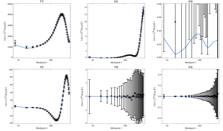
Figure 1: Blind reconstructed CMB power spectra (crosses), $C_{\ell}^{TT}$, $C_{\ell}^{EE}$, $C_{\ell}^{BB}$, $C_{\ell}^{TE}$, $C_{\ell}^{TB}$ and $C_{\ell}^{EB}$, in $\mu{\rm K}_{\rm CMB}^{2}$, at 100 GHz for the [planck c] simulations. We overplot in blue the input model. Error bars are computed using a total of 300 simulations.

Figure 1 shows the blind reconstructed CMB temperature and polarization power spectra, in $\mu$K${}^{2}_{\rm CMB}$, for the 100 GHz channel (crosses). The input model is overplotted in blue. The mean and the error bars are computed from the analysis of 300 simulations.

We observe that $C^{TE}_{\ell}$, $C^{TB}_{\ell}$ and $C^{EB}_{\ell}$ are recovered with no bias, up to $\ell=383$, which is the largest accessible $\ell$ value at $n_{\rm nside}=128$. In the same way, $C^{EE}_{\ell}$ is accurately reconstructed except for the very high $\ell$ values for which pixelization problems may appear (see section 5.3). We also reconstruct efficiently $C^{TT}_{\ell}$ although a small bias (below 10 %) is introduced at low $\ell$ mainly due to confusion with the synchrotron emission as discussed in the following. The $C^{BB}_{\ell}$ spectrum is not recovered at all and a significant bias is observed. This bias, due mainly to statistical residual noise as discussed in the following section, depends only on the signal to noise ratio and does not affect the reconstruction of the other components.

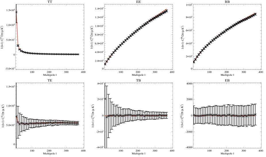
Figure 2: Blind reconstructed simplified-dust emission power spectra, $C_{\ell}^{TT}$, $C_{\ell}^{EE}$, $C_{\ell}^{BB}$, $C_{\ell}^{TE}$, $C_{\ell}^{TB}$ and $C_{\ell}^{EB}$, in $\mu K_{\rm CMB}^{2}$ , at 353 GHz for the [planck c] simulations. We overplot in red the input model. Error bars are computed using a total of 300 simulations.

Figure 2 shows the reconstructed simplified-dust emission power spectra, $C_{\ell}^{TT}$, $C_{\ell}^{EE}$, $C_{\ell}^{BB}$, $C_{\ell}^{TE}$, $C_{\ell}^{TB}$ and $C_{\ell}^{EB}$, in $\mu K_{\rm CMB}^{2}$, at 353 GHz. For comparison we overplot in red the input model. The mean and the error bars displayed were computed using a total of 300 simulations. The reconstruction is fully efficient for $C^{TT}_{\ell}$, $C^{TE}_{\ell}$, $C^{TB}_{\ell}$ and $C^{EB}_{\ell}$ up to $\ell=383$. The $C^{EE}_{\ell}$ and $C^{BB}_{\ell}$ are accurately reconstructed except at $\ell>350$ where a small bias (below 10 %) appears. The $TB$ and $EB$ spectra are compatible with zero as expected from the input model. These results are consistent with the fact that the simulated simplified-dust emission dominate the simulated maps at the HFI channels for which the signal to noise ratio is larger.

Finally, we present in figure 3 the blind reconstructed synchrotron power spectra, in $\mu K_{\rm CMB}^{2}$, at 30 GHz. We overplot in green the power spectrum of the input temperature and polarization synchrotron map from Giardino et al. (2002). Here again $C^{EE}_{\ell}$, $C^{BB}_{\ell}$, $C^{TE}_{\ell}$, $C^{TB}_{\ell}$ and $C^{EB}_{\ell}$ are recovered efficiently. A bias at low $\ell$ (below 20 %) is observed for $C^{TT}_{\ell}$. This is due, as discussed in the following, to the slight mixing-up of the synchrotron and CMB emissions in temperature.

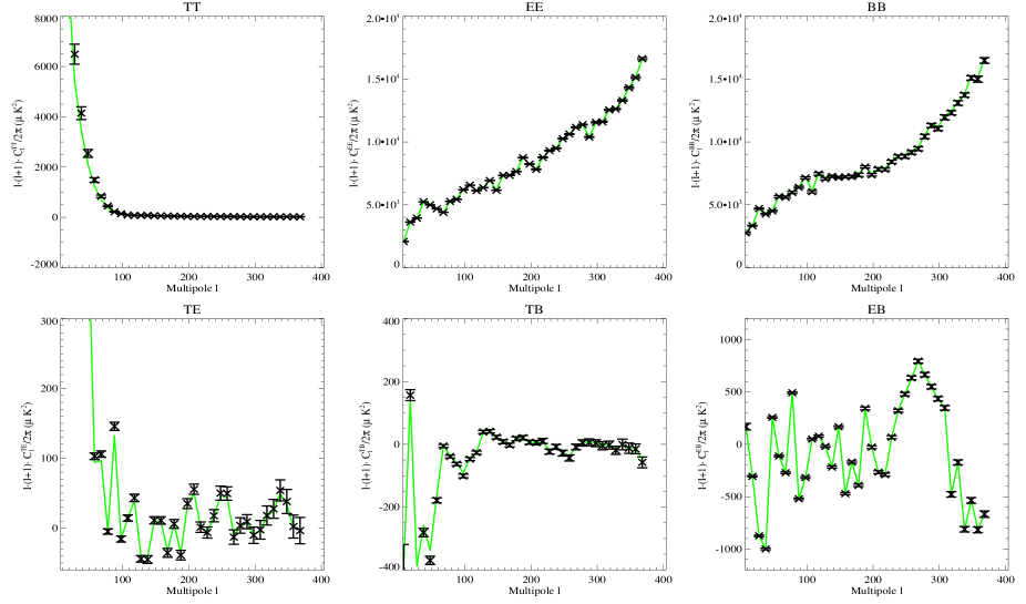
Figure 3: Blind reconstructed synchrotron emission power spectra, $C_{\ell}^{TT}$, $C_{\ell}^{EE}$, $C_{\ell}^{BB}$, $C_{\ell}^{TE}$, $C_{\ell}^{TB}$ and $C_{\ell}^{EB}$, in $\mu K_{\rm CMB}^{2}$ , at 353 GHz. We overplot in green the input model. The error bars are computed using 300 simulations. These are significantly smaller than for the other two components because they do not include cosmic variance. Indeed we use the same synchrotron temperature and polarization maps for all the simulations.

Reconstruction of the mixing matrix

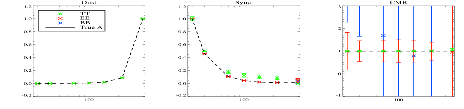
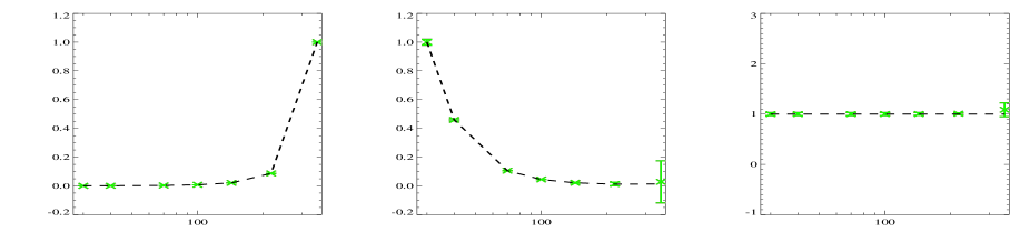
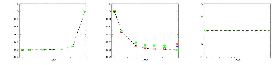
Figure 4: Reconstructed mixing matrix, $A$. Columns, from left to right, correspond to the reconstructed $A$ matrix for dust, synchrotron and CMB respectively. Rows, from top to bottom, correspond to the blind, blind assuming equal temperature and polarization electromagnetic spectrum and the CMB semi-blind analysis of the [planck c] simulations. We display the output electromagnetic spectrum computed for the $T$ (green), $E$ (red) and $B$ (blue) modes as well as the input electromagnetic spectrum (dashed black).

The slight mixing up between synchrotron and CMB is better observed in the reconstructed mixing matrix. The first row of figure 4 shows the blind recovered $A$ matrix for dust, synchrotron and CMB in the case of the [planck c] simulations. The electromagnetic spectrum for $T$, $E$ and $B$ are respectively traced in green, red and blue. For comparison we overplot the input electromagnetic spectrum for each of the components (black dashed line). For convenience we have renormalized the electromagnetic spectrum so that it is unity at 353 GHz, 30 GHz and 100 GHz for dust, synchrotron and CMB respectively. It is important to remark that the reconstruction of the electromagnetic spectra for temperature and polarization is performed independently. We observe that the error bars are larger for polarization than for temperature as we would expect from the smaller signal to noise ratio in polarization.

The simplified-dust electromagnetic spectrum is reconstructed with no bias both in temperature and polarization even at the lowest LFI frequency channels. Furthermore, the reconstructed synchrotron electromagnetic spectra in polarization are not biased. In temperature we observe that the spectrum flattens out at intermediate frequencies between 70 and 217 GHz. This is the cause of the slight mixing up between synchrotron and CMB. This mixing up does not happen in polarization for which the synchrotron emission dominates over the CMB emission. Finally, the reconstruction of the CMB electromagnetic spectrum from the $T$ and $E$ modes, although noisy for the latter, is not biased. However for the $B$ modes the reconstruction is very poor because of the very low signal to noise ratio (below $10^{-2}$ for $\ell>100$).

We have repeated the analysis with no prior in the electromagnetic spectrum of the CMB. We use instead the eigenvector corresponding to the third larger eigenvalue of the data density matrix. The results for dust and synchrotron remain unchanged. For CMB the electromagnetic spectrum at 30 and 353 GHz is not reconstructed neither in temperature nor in polarization and the results for $B$ are significantly degraded at all frequencies. However, the results on the reconstruction of the spatial power spectra remain unchanged for all the physical components including CMB. This can be easily understood as the reconstruction of the CMB power spectra is mainly dominated by the intermediate frequency maps, from 70 to 217 GHz, where the $A$ matrix is accurately reconstructed.

Assuming equal temperature and polarization electromagnetic spectrum

In the previous analysis we have computed the electromagnetic spectrum of the physical components independently for each mode $T$, $E$ and $B$. In a more realistic approach we should consider a single electromagnetic spectrum for the polarization $E$ and $B$ modes which may be different from the temperature one. We have repeated the analysis under the above hypothesis and the results remain roughly the same with respect to the reconstruction of the spatial power spectra and of the electromagnetic spectrum. For synchrotron and simplified-dust the $E$ and $B$ modes have roughly the same power in our simulations and therefore we expect only variations in the error bars. For CMB the $E$ mode largely dominates the $B$ mode and therefore we expect no significant contribution from the latter to the electromagnetic spectrum reconstruction.

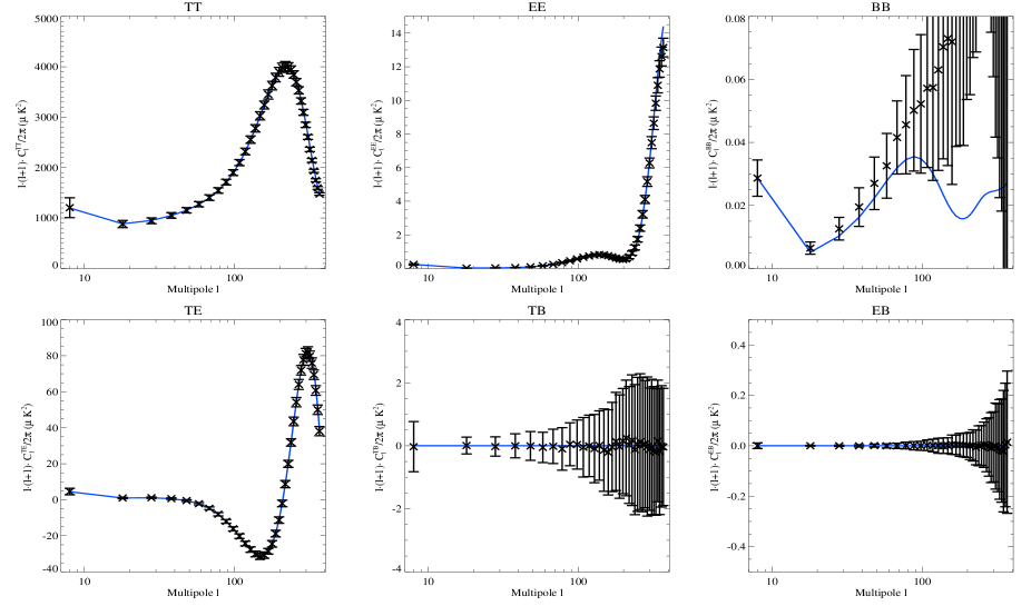
Figure 5: Same as figure 1 except for a blind analysis assuming equal temperature and polarization electromagnetic spectrum.

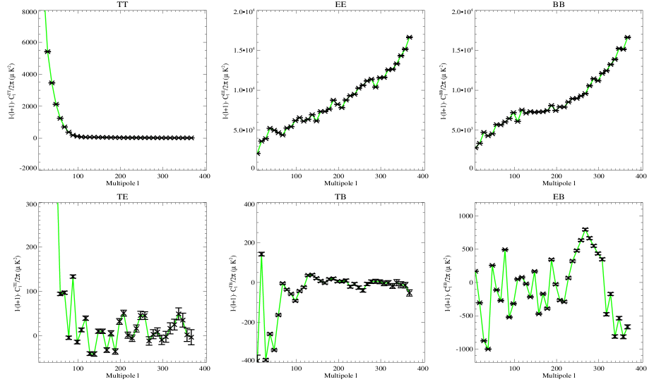
Figure 6: Same as figure 3 but for a blind analysis assuming equal temperature and polarization electromagnetic spectrum.

The differences between the temperature and polarization electromagnetic spectra are expected to be small for dust and synchrotron Planck Consortium (2005) and none for the CMB Zaldarriaga & Seljak 1997 . Therefore, in the case of a perfectly calibrated experiment, we can consider, in a first approximation, that the polarization and the temperature electromagnetic spectra are the same. The blind analysis of the [planck c] simulations under this hypothesis shows no evidence of mixing up between synchrotron and CMB. This can be clearly observed in the second row of figure 4 where we represent from left to right the reconstructed electromagnetic spectrum of the dust, synchrotron and CMB emissions respectively. No bias is observed for any of the physical components including synchrotron for which the flatten out of the spectrum observed before is not present.

Figures 5 and 6 show the CMB and synchrotron reconstructed spatial power spectra in temperature and polarization. We do not observe a bias neither on the synchrotron nor on the CMB $TT$ power spectra. Furthermore, we observe that the CMB $BB$ modes, although biased at large $\ell$ values, are fairly reconstructed up to $\ell=60$. For the other modes, the results are similar to those presented in the previous section.

5.2 Semi-blind separation

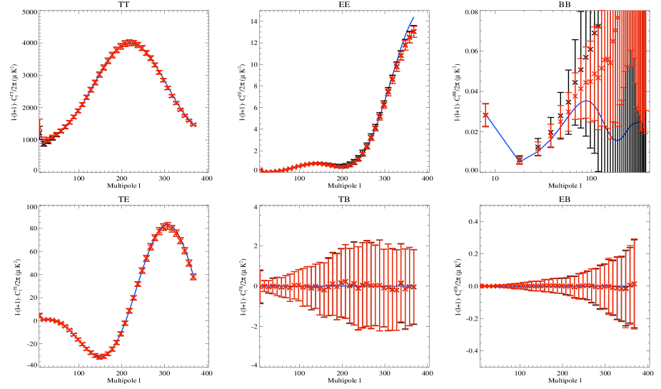
Figure 7: Same as figure 1 but for a CMB semi-blind (black) and A-fixed (red) analysis (see text for details).

The separation method allows us to easily include previous knowledge on the physical components either as priors or as facts. In the previous section we considered a prior on the CMB emission. In the following we move a step forward in the analysis assuming the CMB electromagnetic spectrum known and performing what we call a CMB semi-blind analysis. For this analysis, the columns of the mixing matrix corresponding to the CMB are initialized to the CMB electromagnetic spectrum and are not updated by the algorithm. For the other components we consider independent electromagnetic spectra for temperature and polarization and they are initialized as for the blind analysis.

The third row of figure 4 shows the reconstructed mixing matrix for the CMB semi-blind analysis considering the [planck c] simulations. The results are similar to those of the blind analysis discussed before. The dust electromagnetic spectrum is accurately recovered in temperature and polarization. For synchrotron, the polarization spectrum is accurately recovered but the temperature one flattens out at intermediate frequencies with respect to the input model. Therefore, the reconstructed simplified-dust and synchrotron spatial power spectra in temperature and polarization are similar to those of the blind analysis. The simplified-dust power spectra are accurately reconstructed in temperature and polarization. For synchrotron the power spectra are also accurately reconstructed except for the $TT$ mode which present a slight bias (below 20%) at large angular scales ($\ell<60$). In general the error bars are smaller for the CMB semi-blind analysis.

The reconstructed CMB power spectra for the CMB semi-blind analysis are represented in black on figure 7. All of them are accurately reconstructed with no bias except for the $BB$ mode. For the latter the reconstruction is accurate up to $\ell=60$ and there on is biased. This bias is due to residual noise and is not related to the uncertainties on the reconstruction of the electromagnetic spectrum for the other physical components. To check this we have also performed a A-fixed analysis assuming the electromagnetic spectrum of all physical components known. The results of this analysis are overplotted in red on the figure. We observe that reconstruction is equivalent to that of the CMB semi-blind analysis but for the error bars which are smaller This indicates that the bias in the $BB$ mode is mainly due to residual noise as discussed in section 5.4.

5.3 Reconstruction of the small angular scales

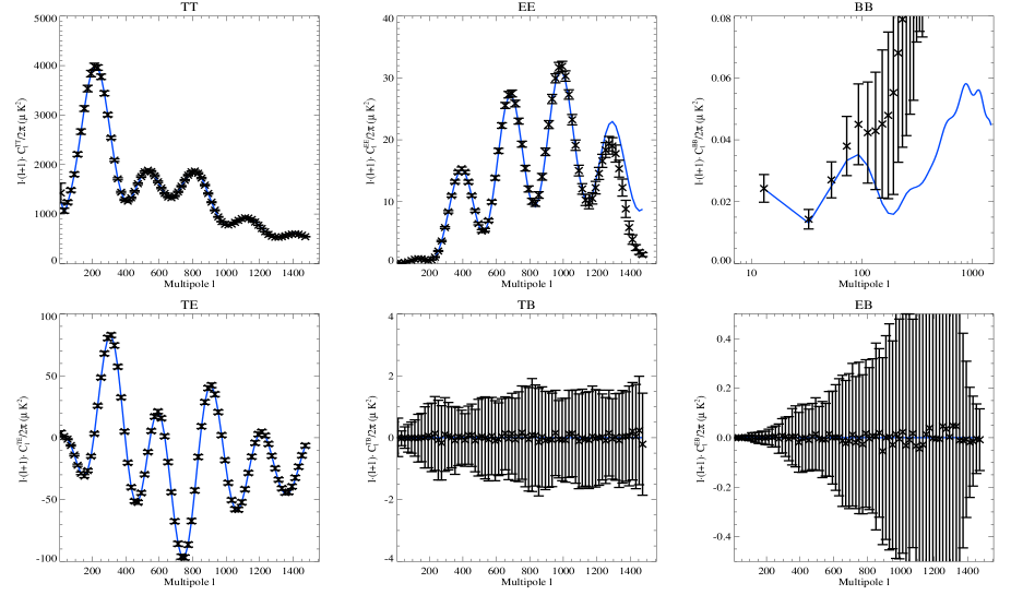
Figure 8: Same as figure 1 but for the [planck a] simulations for a CMB semi-blind analysis.

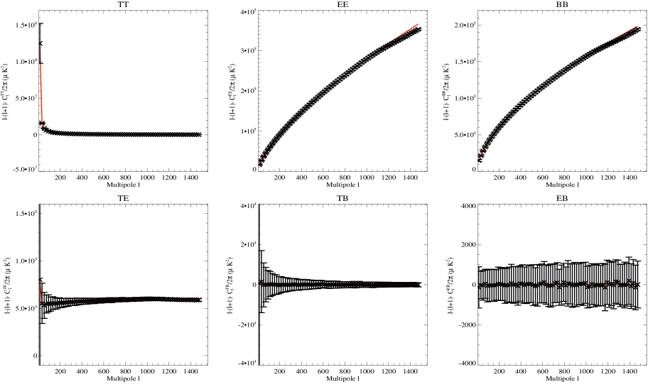
Figure 9: Same as figure 2 but for the [planck a] simulations for a CMB semi-blind analysis.

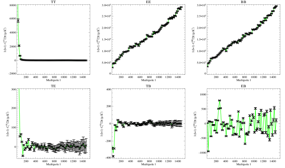
Figure 10: Same as figure 3 but for the [planck a] simulations for a CMB semi-blind analysis.

In the previous section we have fully described the analysis of the [planck c] simulations at $n_{\rm side}=128$ for which the reconstruction of the spatial power spectra was limited to $\ell=383$. In some cases we have observed small biases in the polarization auto power spectra at large $\ell$ values which may be due to pixelization problems (we exclude in here the bias observed in the CMB $BB$ modes which is due to residual noise). To check this hypothesis we have also performed the blind, CMB semi-blind and A-fixed analysis on the [planck a] simulations for which we can reconstruct the angular power spectra up to $\ell=1535$. As the resolution of the Planck best channels is $\sim 5$ arcmin a more realistic analysis will require simulations at $n_{side}=2048$ which are far too much time demanding for our computational capabilities.

The results obtained for the [planck a] simulations are very similar to those for the [planck c] ones. For illustration figures 8, 9 and 10 show the reconstructed temperature and polarization power spectra for CMB, simplified-dust and synchrotron in the case of a CMB semi-blind analysis. The synchrotron and simplified-dust power spectra are accurately reconstructed in temperature and polarization. We observe a slight bias in the dust $EE$ and $BB$ modes as for the [planck c] simulations but at much larger $\ell$ values. This indicates that this bias is related to pixelization effects. The same effect is observed for the CMB power spectra. The bias in the $EE$ modes is present at much larger $\ell$ than for the [planck c] simulations. The reconstruction of the CMB $BB$ modes is accurate at low $\ell$ ($\ell<60$) and present a residual noise bias at large $\ell$ values as discussed in the previous section.

5.4 Color noise model

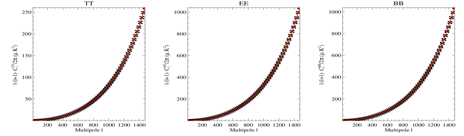
Figure 11: Reconstructed noise angular auto power spectra (black), in $\mu{\rm K}_{\rm CMB}^{2}$, at 100 GHz for $T$, $E$ and $B$ for the [planck a] simulations in the case of a CMB semi-blind separation. We overplot in red the noise auto power spectra at 100 GHz as obtained from 100 realizations of noise-only maps.

As seen before, the bias observed in the CMB $BB$ power spectrum is most probably due to residual noise from the separation. Therefore, it is interesting to check both the accuracy of the noise reconstruction and the limitations of the white noise model imposed. With respect to the latter we have repeated all the analysis presented above assuming a color noise model such that the noise power spectra are estimated for each bin $b$ in $\ell$. For the blind analysis the results are slightly worse in the sense that the mixing up between CMB and synchrotron is more significant. This is not surprising since the noise in the data is white and we are artificially reducing the number of degrees of freedom in the fit. Actually, the mismatch between the data and the physical component power spectra can be compensated by changing the noise power spectra. In the case of the CMB semi-blind and A-fixed analysis the results for the white and color noise model present no significant differences.

Figure 11 shows, in black, the reconstructed noise angular power spectra, $C_{\ell}^{N,TT}$, $C_{\ell}^{N,EE}$, $C_{\ell}^{N,BB}$, in $\mu{\rm K}_{\rm CMB}^{2}$, at 100 GHz for the [planck a] simulations in the case of a CMB semi-blind analysis. We overplot, in black, the power spectra of the noise at 100 GHz obtained from 100 realizations of noise-only maps. The noise spectra are reconstructed down to the accuracy of the estimation of the input model both for $TT$ and $EE$, well below 10^-3 %. For the $BB$ noise spectrum there is a small bias which is of the order of $5\times 10^{-3}$ % at $\ell=200$ and around $2\times 10^{-2}$ % at $\ell=1500$.

Therefore, to improve the reconstruction of the CMB $BB$ modes we need a better estimation of the $BB$ noise power spectrum. For this purpose we need to improve the likelihood maximization algorithm. For temperature-only separation, Delabrouille et al. 2003 complemented the EM algorithm with a direct maximization of the likelihood function via a Newton-Raphson algorithm. For polarization similar algorithms can be used but due to the degree of complexity of the problem (6 correlated modes per physical component instead of 1 in the temperature only case) and for the sake of clarity these will be discussed in a forthcoming paper.

6 Towards a more realistic sky model

After testing intensively our algorithm on our simplified model, deducting the global performances of the spectral matching reconstruction in temperature and polarization we are interested in the performances of the algorithm for significantly spatially correlated components. For this purpose, we have used the [planck d] simulations.

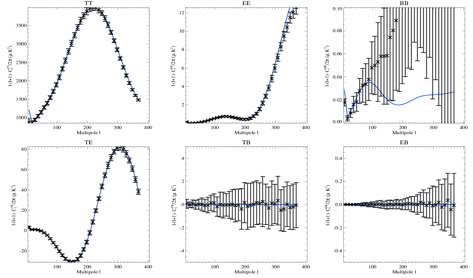
Figure 12: A-fixed reconstruction o the CMB $C_{\ell}^{TT}$, $C_{\ell}^{EE}$, $C_{\ell}^{BB}$, $C_{\ell}^{TE}$, $C_{\ell}^{TB}$ and $C_{\ell}^{EB}$ power spectra (crosses), in $\mu{\rm K}_{\rm CMB}^{2}$, at 100 GHz in the case of the realistic model with 4 components. We overplot in blue the input model. Error bars are computed using a total of 100 simulations.

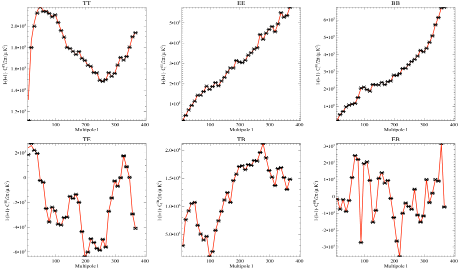
Figure 13: A-fixed reconstruction of the realistic dust $C_{\ell}^{TT}$, $C_{\ell}^{EE}$, $C_{\ell}^{BB}$, $C_{\ell}^{TE}$, $C_{\ell}^{TB}$ and $C_{\ell}^{EB}$ power spectra (crosses), in $\mu{\rm K}_{\rm CMB}^{2}$, at 353 GHz in the case of the realistic model with 4 components. We overplot in red the input model. Error bars are computed using a total of 100 simulations.

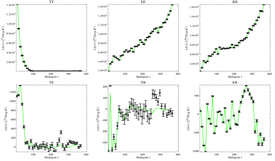
Figure 14: A-fixed reconstruction of the synchrotron emission $C_{\ell}^{TT}$, $C_{\ell}^{EE}$, $C_{\ell}^{BB}$, $C_{\ell}^{TE}$, $C_{\ell}^{TB}$ and $C_{\ell}^{EB}$ power spectra (crosses), in $\mu{\rm K}_{\rm CMB}^{2}$, at 30 GHz in the case of the realistic model with 4 components. We overplot in green the input model. Error bars are computed using a total of 100 simulations.

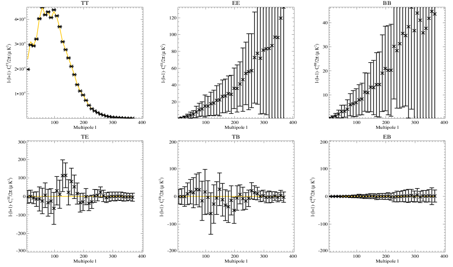
Figure 15: A-fixed reconstruction of the free-free emission $C_{\ell}^{TT}$, $C_{\ell}^{EE}$, $C_{\ell}^{BB}$, $C_{\ell}^{TE}$, $C_{\ell}^{TB}$ and $C_{\ell}^{EB}$ power spectra (crosses), in $\mu{\rm K}_{\rm CMB}^{2}$, at 30 GHz in the case of the realistic model with 4 components. We overplot in orange the input model. Error bars are computed using a total of 100 simulations.

With this set of simulations, we have performed several types of separations. First, we have worked on a joint temperature and polarization analysis, similar to the one presented in section 5. Then we have considered temperature-only separation, and polarization-only separation. For each of the described cases we have applied the algorithm with the different degrees of freedom presented in section 5.

Models and recovered data are average over bins of size 10 in $\ell$ beginning at $\ell=3$. Error bars presented in this section represent the dispersion over 100 simulations. Note that $n_{\rm side}=128$ allows a theoretical reconstruction up to $\ell=383$ in temperature and $\ell\sim 256$ in polarization Górski et al. (1999). CMB recovered spectra are plotted at 100 GHz while dust at 353 GHz and synchrotron and free-free at 30 GHz.

6.1 Joint temperature and polarization separation

We have first performed a joint temperature and polarization separation on the realistic model. We present here the results obtained in the A-fixed separation case, considering the 4 simulated components. In this particular case, the algorithm is very slow to converge and thus 40000 EM iterations have been run. The recovered angular power spectra for temperature and polarization are displayed from figure 12 to figure 15, respectively for CMB, realistic dust, synchrotron and free-free emissions and compared to the input model.

For the CMB component, on figure 12 we can see that $C_{\ell}^{TT}$ and $C_{\ell}^{TE}$ are recovered accurately up to $\ell\sim 400$. Recovered spectra for $C_{\ell}^{TB}$ and $C_{\ell}^{EB}$ are compatible with zero as expected. $C_{\ell}^{EE}$ is recovered with a good accuracy up to $\ell\sim 250$ and then is slightly biased due to pixelization problems in the HEALPix scheme. Finally, the $C_{\ell}^{BB}$ spectrum is recovered up to $\ell\sim 90$ and then is biased with residual noise as discussed in section 5.4.

The Realistic dust component recovered spectra are displayed on figure 13. We can see that $C_{\ell}^{TT}$, $C_{\ell}^{EE}$, $C_{\ell}^{BB}$, $C_{\ell}^{TE}$, $C_{\ell}^{TB}$ and $C_{\ell}^{TT}$ are recovered with a perfect accuracy up to $\ell=383$.

The recovered power spectra for the synchrotron component are displayed on figure 14. Polarization only power spectra ($C_{\ell}^{EE}$, $C_{\ell}^{BB}$ and $C_{\ell}^{EB}$) are recovered in good agreement with the input model. $C_{\ell}^{TT}$ is well recovered up to $\ell\sim 200$ but then converge sharply to a null signal and therefore a residual noise bias similar to the one of $C_{\ell}^{BB}$ occurs. This is not directly visible in the temperature spectrum but can be seen in the cross temperature and polarization spectra. Indeed, $C_{\ell}^{TE}$ and $C_{\ell}^{TB}$ are well recovered up to $\ell\sim 200$ and further many points are strongly biased.

Finally, results corresponding to the free-free emission component are displayed in figure 15. $C_{\ell}^{TT}$ is recovered with a good accuracy up to $\ell=383$. As for polarization the input signal is null, we can see in the recovered spectra the overall behavior of our algorithm described in section 5.

The algorithm has also been run for CMB-fixed and Blind separations. For both of them, excepting the dust component which is well constrained in all cases due to its dominant power at high frequencies, the algorithm fails to converge and then components are mixed and results strongly biased. This may come from the fact that free-free and synchrotron electromagnetic spectra are similar and to the fact that all the Galactic emissions have strong spatial correlations. In the following section we will address this problem and show that this mixing that prevents the convergence of the algorithm is mainly due to the separability problem that occurs in temperature. In section 6.3, we will see that the separation performed on sets of $Q$ and $U$ maps has not this separability problem.

Notice that when not considering the free-free emission in the simulations, results are very similar and the same performances of the algorithm with respect to the level of prior we assume are observed.

6.2 Temperature-only separation

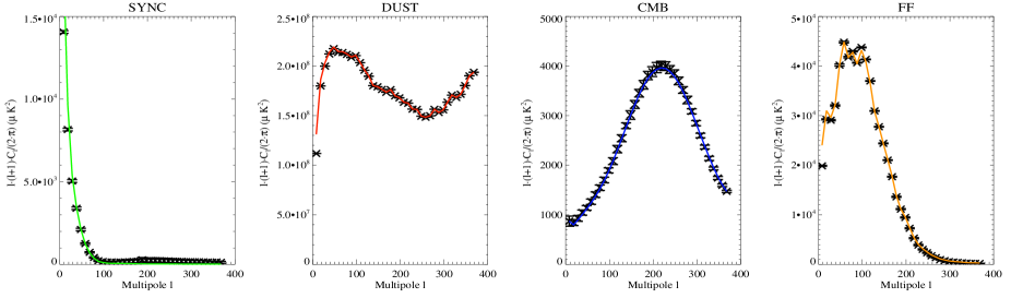
Figure 16: A-fixed temperature-only reconstruction of the $C_{\ell}^{TT}$ power spectra (crosses) in $\mu{\rm K}_{\rm CMB}^{2}$ in the case of the realistic model with 4 components. Results are displayed from left to right for the 4 different components, i.e synchrotron (at 30 GHz), realistic dust (at 353 GHz), CMB (at 100 GHz) and free-free (at 30 GHz). Input models are overplotted in solid lines. Error bars are computed using a total of 100 simulations.

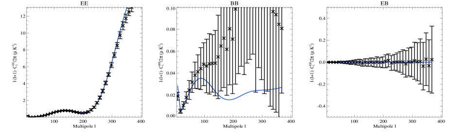
Figure 17: A-fixed polarization-only reconstruction of the CMB $C_{\ell}^{EE}$, $C_{\ell}^{BB}$ and $C_{\ell}^{EB}$ power spectra (crosses) in $\mu{\rm K}_{\rm CMB}^{2}$ at 100 GHz in the case of the realistic model with 3 polarized components. Input models are overplotted in blue. Error bars are computed using a total of 100 simulations.

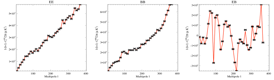
Figure 18: A-fixed polarization-only reconstruction of the realistic dust $C_{\ell}^{EE}$, $C_{\ell}^{BB}$ and $C_{\ell}^{EB}$ power spectra (crosses) in $\mu{\rm K}_{\rm CMB}^{2}$ at 353 GHz in the case of the realistic model with 3 polarized components. Input models are overplotted in red. Error bars are computed using a total of 100 simulations.

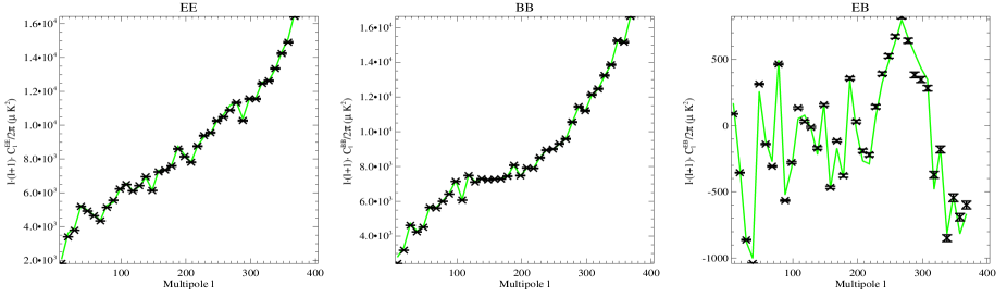
Figure 19: A-fixed polarization-only reconstruction of synchrotron emission $C_{\ell}^{EE}$, $C_{\ell}^{BB}$ and $C_{\ell}^{EB}$ power spectra (crosses) in $\mu{\rm K}_{\rm CMB}^{2}$ at 30 GHz in the case of the realistic model with 3 polarized components. Input models are overplotted in green. Error bars are computed using a total of 100 simulations.

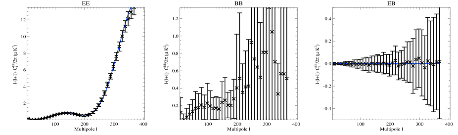
Figure 20: Blind polarization-only reconstruction of the CMB $C_{\ell}^{EE}$, $C_{\ell}^{BB}$ and $C_{\ell}^{EB}$ power spectra (crosses) in $\mu{\rm K}_{\rm CMB}^{2}$ at 100 GHz in the case of the realistic model with 3 polarized components. Input models are overplotted in blue. Error bars are computed using a total of 100 simulations.

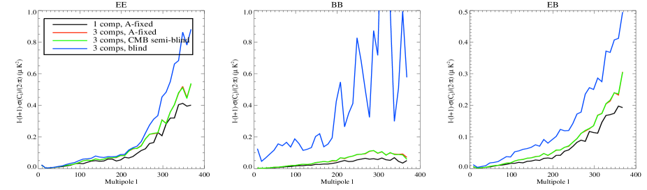
Figure 21: Error bars of the reconstruction of the CMB $C_{\ell}^{EE}$, $C_{\ell}^{BB}$ and $C_{\ell}^{EB}$ power spectra in $\mu{\rm K}_{\rm CMB}^{2}$ at 100 GHz in a Blind (blue), CMB semi-blind (green) and A-fixed separations of a 3 components mixture containing CMB, realistic dust and synchrotron and in a A-fixed separation of a set CMB and noise only simulations (black).

We have performed a temperature-only separation on the realistic model. For this we consider sets of $I$ maps and the algorithm solve the spectral matching equations for $T$ modes only, like in the SMICA algorithm Delabrouille et al. 2003 . We present here the results obtained in the A-fixed separation case, considering the 4 simulated components.

Recovered $C_{\ell}^{TT}$ spectra are displayed in figure 16 for synchrotron, realistic dust, CMB and free-free. We can see that except the synchrotron spectrum which start to be biased at $\ell\sim 200$, for the reason advanced in the last section, spectra are recovered with a good accuracy for the dust, CMB and free-free components up to $\ell=383$. We have also performed the separation for the CMB-fixed and the Blind cases. As for the joint analysis, excepting again the dust component for which the spectrum is recovered efficiently, the algorithm fails to converge. Note that in the literature, no method has successfully separated synchrotron from dust on a noisy simulated mixture of CMB and astrophysical foregrounds, working on all sky maps.

Comparable results and the same performances of the algorithm with respect to the level of prior we assume are observed when no free-free component is included in simulations.

6.3 Polarization-only separation

Finally, we have performed a polarization-only separation on the realistic model. For this we consider sets of $Q$ and $U$ maps and the algorithm solve the spectral matching equations for $E$ and $B$ modes (allowing reconstruction of $C_{\ell}^{EE}$, $C_{\ell}^{BB}$ and $C_{\ell}^{EB}$). Notice that as we suppose that the free-free emission is not polarized, the sets of polarized maps used here only contain CMB, realistic dust, synchrotron and noise.

CMB semi-blind separation

We have performed a CMB semi-blind separation on the polarization-only set of maps. In this case, the CMB electromagnetic spectrum is initialized to 1 and kept fixed (see section 5).

The results of this analysis on the CMB power spectra are displayed in figure 17. We can see that $C_{\ell}^{EE}$ are reconstructed without bias up to $\ell\sim 300$, as expected with this pixelization scheme and that $C_{\ell}^{EB}$ is compatible with zero. $C_{\ell}^{BB}$ is efficiently recovered up to $\ell\sim 50$ and then is biased with residual noise from the separation.

The realistic dust and synchrotron emissions recovered power spectra are displayed in figure 18 and 19. In both cases we can see that $C_{\ell}^{EE}$, $C_{\ell}^{BB}$ and $C_{\ell}^{EB}$ are reconstructed very efficiently up to $\ell=383$.

Blind separation

We have also performed, for the polarization-only separation, a Blind separation. The results of this analysis for dust and synchrotron are not displayed, but for both, $C_{\ell}^{EE}$, $C_{\ell}^{BB}$ and $C_{\ell}^{EB}$ are reconstructed very efficiently up to $\ell=383$. The reconstruction of the CMB component is displayed in figure 20. For $C_{\ell}^{EE}$ we can see that the reconstruction is similar to the one in the CMB semi-blind case, only the error bars are larger. However, the $C_{\ell}^{BB}$ spectrum is not recovered.

6.4 Discussions

From the previous analyzes we have clearly identified a separability problem when dealing with more than one realistic diffuse Galactic emission component. This problem appears both in the joint temperature and polarization and in the temperature-only analyzes, but not in the polarization-only one. This would indicate that it is mainly due to the high level of correlation of the Galactic diffuse emission in temperature both in the Galactic plane and at high Galactic latitudes. The current version of our algorithm assume uncorrelated components and therefore we expect it to behave badly when they are correlated. Work is in progress to adapt PolEMICA to account for spatially correlated components.

For polarization-only separation the correlation problem seems to be not significant and the CMB semi-blind and blind analyzes are possible. Therefore, for this case, we can evaluate the loss of accuracy in the reconstruction of the CMB signal due to the foreground contamination. For this, we compare the error bars on the CMB power spectra for the A-fixed, CMB semi-blind and blind separations to the one obtained in the case of a A-fixed separation on [planck b] simulations containing CMB and noise only.

Results are presented in figure 21. $C_{\ell}^{EE}$, $C_{\ell}^{BB}$ and $C_{\ell}^{EB}$ reconstruction error bars behave similarly with respect to the different algorithm priors. For each of them, A-fixed and CMB semi-blind error bars are of the same amplitude and are between 25 and 50 % larger (respectively a factor 1.26 for $C_{\ell}^{EE}$, 1.50 for $C_{\ell}^{BB}$ and 1.29 for $C_{\ell}^{EB}$) than the reference A-fixed CMB only case. This means that in the context of our realistic model, we have no need to put priors on the foregrounds electromagnetic spectra in polarization to perform an efficient separation. In the Blind case, error bars of the reconstruction are increased by a factor 1.59 for $C_{\ell}^{EE}$, 13.5 for $C_{\ell}^{BB}$ (but the reconstruction is biased) and 2.52 for $C_{\ell}^{EB}$. On the other hand, these results stress the fact that having priors on the CMB electromagnetic spectra inside of our algorithm helps to perform a more accurate separation.

7 Summary and conclusions

We present in this paper the PolEMICA algorithm which is an extension to polarization of the SMICA temperature MD-MC blind component separation method developed by Delabrouille et al. 2003 . Both algorithms work in harmonic space and are based on the spectral matching of the data to a noisy linear mixture of uncorrelated physical components using the EM algorithm to maximize the likelihood function. By contrast to the temperature data which are described by a single scalar quantity $T$, the combined temperature and polarization data are described in harmonic space by three correlated scalar quantities $T$, $E$ and $B$ corresponding to the $I$, $Q$ and $U$ Stokes parameters in real space. We have developed a new formalism to jointly deal with the 6 resulting auto and cross angular power spectra, $TT$, $EE$, $BB$, $TE$, $TB$ and $EB$.

Using this formalism we have constructed the likelihood function and proved that the EM algorithm can be also applied to polarization data. Under the assumption of uncorrelated Gaussian distributed components and noise, the free parameters in the fit are the mixing matrix describing the electromagnetic spectrum of the physical components for $T$, $E$ and $B$, the temperature and polarization angular power spectra of the physical components and the temperature and polarization noise power spectra for each of the detectors.

We have, as a first approach, intensively and successfully tested the PolEMICA method on simulations of the Planck satellite experiment considering a 14-months nominal mission and no systematic effects. For these tests, we suppose a simplified linear model for the sky emission including CMB, synchrotron with constant spectral index and simplified-dust (Gaussian realization) emissions. We construct full sky maps for all the polarized channels from 30 to 353 GHz including at least one of the above physical components and considering white noise and infinite resolution.

The method permits blind separation on these simulations allowing us to reconstruct the noise and physical component’s temperature and polarization power spectra as well as the mixing matrix when we consider equal electromagnetic spectrum in $T$, $E$ and $B$. When we relax this hypothesis the reconstruction of the electromagnetic spectrum for the CMB $B$ modes is significantly degraded as could be expected because of the low signal to noise ratio. These results indicate that the PolEMICA method allows us to both constrain the electromagnetic spectrum of the physical components and also to inter-calibrate the data based on the reconstructed CMB electromagnetic spectrum.

After setting the general performances of the algorithm, we have performed the separation on a more realistic model that includes realistic-dust, synchrotron and free-free components in section 6. We have encountered in this case a separability problem, that mixes up components and prevents the algorithm to converge, when performing blind separations. We have shown that this is due to spatial correlations between Galactic components in temperature. Thus, when working on sets of $Q$ and $U$ maps and maximizing the likelihood for $EE$, $BB$ and $EB$ modes only, this separability problem does not occur and CMB semi-blind and blind separations are possible. For this polarization-only case, we have shown that considering our realistic sky model and our algorithm, in the Planck case, we have no need to put priors on the Galactic components electromagnetic spectra to reconstruct the CMB polarized power spectra. Nevertheless, adding priors on the CMB electromagnetic spectrum helps to perform a more accurate separation.

Finally, real experiments present finite resolution, partial effective sky coverage, systematic effects and, often, correlated noise. All these issues must be dealt with by the component separation algorithms and will with no doubt significantly limit the precision to which the CMB signal may be reconstructed. PolEMICA, as it was already the case for SMICA, can account for beam and filtering smoothing. Systematic effects and correlated noise can be modeled as extra components in the data for which the spectral dependence can be estimated in a blind analysis. Moreover, the strong spatial correlation in temperature between Galactic physical emissions: dust, synchrotron and free-free, is a major problem for blind component separation algorithms which generally assumed uncorrelated components. Although not observed yet, we can also imagine spatial correlation of the Galactic emissions in polarization. Work is in progress to adapt the PolEMICA algorithm to the case of correlated components.

In addition, foreground emissions have in general spatially varying electromagnetic spectra far beyond the simple linear model presented here. Work is also in progress to adapt PolEMICA to the case of foregrounds with spatially varying electromagnetic spectrum.

Appendix A MD-MC Polarization sky model

We discuss here the formalism developed to describe the temperature and polarization observations as a noisy mixture of independent components.

In the following we assume full sky observations at two frequencies $\nu_{1}$ and $\nu_{2}$ and a simple linear model for the sky emission with two components $c_{1}$ and $c_{2}$.

In this case, equation (2) reads

$$\left(\begin{array}[]{c}y^{\nu_{1}T}_{\ell m}\\ y^{\nu_{1}E}_{\ell m}\\ y^{\nu_{1}B}_{\ell m}\\ y^{\nu_{2}T}_{\ell m}\\ y^{\nu_{2}E}_{\ell m}\\ y^{\nu_{2}B}_{\ell m}\end{array}\right)=\left(\begin{array}[]{cccccc}f^{T}_{\nu_{1}c_{1}}&0&0&f^{T}_{\nu_{1}c_{2}}&0&0\\ 0&f^{E}_{\nu_{1}c_{1}}&0&0&f^{E}_{\nu_{1}c_{2}}&0\\ 0&0&f^{B}_{\nu_{1}c_{1}}&0&0&f^{B}_{\nu_{1}c_{2}}\\ f^{T}_{\nu_{2}c_{1}}&0&0&f^{T}_{\nu_{2}c_{2}}&0&0\\ 0&f^{E}_{\nu_{2}c_{1}}&0&0&f^{E}_{\nu_{2}c_{2}}&0\\ 0&0&f^{B}_{\nu_{2}c_{1}}&0&0&f^{B}_{\nu_{2}c_{2}}\end{array}\right)\cdot\left(\begin{array}[]{c}s^{c_{1}T}_{\ell m}\\ s^{c_{1}E}_{\ell m}\\ s^{c_{1}B}_{\ell m}\\ s^{c_{2}T}_{\ell m}\\ s^{c_{2}E}_{\ell m}\\ s^{c_{2}B}_{\ell m}\end{array}\right)+\left(\begin{array}[]{c}n^{\nu_{1}T}_{\ell m}\\ n^{\nu_{1}E}_{\ell m}\\ n^{\nu_{1}B}_{\ell m}\\ n^{\nu_{2}T}_{\ell m}\\ n^{\nu_{2}E}_{\ell m}\\ n^{\nu_{2}B}_{\ell m}\end{array}\right)$$

where $y^{\nu_{i}X}_{\ell m}$ and $s^{c_{j}X}_{\ell m}$ for $X=\{T,E,B\}$ are the coefficients of the spherical harmonic decomposition of the input sky observations and of the components of the sky model respectively. The coefficients $f^{X}_{\nu_{i}c_{j}}$ correspond to the electromagnetic spectrum of the component $c_{j}$ at the frequency of observation $\nu_{i}$. Note that the mixing matrix, $A$, has dimensions $3\cdot n_{\nu}\times 3\cdot n_{c}$.

We define the noise, $R_{n}(b)$, signal, $R_{s}(b)$, and data, $R_{y}(b)$, density matrices used in equation (5) for each bin, $b$, as follows

$$R_{z}(b)\equiv\frac{1}{n_{b}}\sum_{\vec{\ell}\in\mathcal{D}_{b}}<z(\vec{\ell})z(\vec{\ell})^{\dagger}>\ ,\qquad z=\{n,s,y\}$$

Assuming the noise uncorrelated between detectors the noise density matrix is diagonal

$$R_{n}(b)=\left(\begin{array}[]{ccc}&\nu_{1}&\nu_{2}\\ \nu_{1}&\begin{array}[]{ccc}N_{\ell}^{TT}(b)&&\\ &N_{\ell}^{EE}(b)&\\ &&N_{\ell}^{BB}(b)\\ \end{array}&\begin{array}[]{ccc}&&\\ &0&\\ &&\\ \end{array}\\ \nu_{2}&\begin{array}[]{ccc}&&\\ &0&\\ &&\\ \end{array}&\begin{array}[]{ccc}N_{\ell}^{TT}(b)&&\\ &N_{\ell}^{EE}(b)&\\ &&N_{\ell}^{BB}(b)\\ \end{array}\\ \end{array}\right)$$

In the same way assuming independent physical components the signal density matrix is block diagonal and reads

$$R_{s}(b)=\left(\begin{array}[]{ccc}&c_{1}&c_{2}\\ c_{1}&\left[\begin{array}[]{ccc}S_{\ell}^{TT}(b)&S_{\ell}^{TE}(b)&S_{\ell}^{TB}(b)\\ S_{\ell}^{TE}(b)&S_{\ell}^{EE}(b)&S_{\ell}^{EB}(b)\\ S_{\ell}^{TB}(b)&S_{\ell}^{EB}(b)&S_{\ell}^{BB}(b)\\ \end{array}\right]&\begin{array}[]{ccc}&&\\ &0&\\ &&\\ \end{array}\\ c_{2}&\begin{array}[]{ccc}&&\\ &0&\\ &&\\ \end{array}&\left[\begin{array}[]{ccc}S_{\ell}^{TT}(b)&S_{\ell}^{TE}(b)&S_{\ell}^{TB}(b)\\ S_{\ell}^{TE}(b)&S_{\ell}^{EE}(b)&S_{\ell}^{EB}(b)\\ S_{\ell}^{TB}(b)&S_{\ell}^{EB}(b)&S_{\ell}^{BB}(b)\\ \end{array}\right]\\ \end{array}\right)$$

Finally the data density matrix can written by blocks as follows

$$R_{y}(b)=\left(\begin{array}[]{ccc}&\nu_{1}&\nu_{2}\\ \nu_{1}&\left[\begin{array}[]{ccc}Y_{\ell}^{TT}(b)&Y_{\ell}^{TE}(b)&Y_{\ell}^{TB}(b)\\ Y_{\ell}^{TE}(b)&Y_{\ell}^{EE}(b)&Y_{\ell}^{EB}(b)\\ Y_{\ell}^{TB}(b)&Y_{\ell}^{EB}(b)&Y_{\ell}^{BB}(b)\\ \end{array}\right]&\left[\begin{array}[]{ccc}Y_{\ell}^{TT}(b)&Y_{\ell}^{TE}(b)&Y_{\ell}^{TB}(b)\\ Y_{\ell}^{TE}(b)&Y_{\ell}^{EE}(b)&Y_{\ell}^{EB}(b)\\ Y_{\ell}^{TB}(b)&Y_{\ell}^{EB}(b)&Y_{\ell}^{BB}(b)\\ \end{array}\right]\\ \nu_{2}&\left[\begin{array}[]{ccc}Y_{\ell}^{TT}(b)&Y_{\ell}^{TE}(b)&Y_{\ell}^{TB}(b)\\ Y_{\ell}^{TE}(b)&Y_{\ell}^{EE}(b)&Y_{\ell}^{EB}(b)\\ Y_{\ell}^{TB}(b)&Y_{\ell}^{EB}(b)&Y_{\ell}^{BB}(b)\\ \end{array}\right]&\left[\begin{array}[]{ccc}Y_{\ell}^{TT}(b)&Y_{\ell}^{TE}(b)&Y_{\ell}^{TB}(b)\\ Y_{\ell}^{TE}(b)&Y_{\ell}^{EE}(b)&Y_{\ell}^{EB}(b)\\ Y_{\ell}^{TB}(b)&Y_{\ell}^{EB}(b)&Y_{\ell}^{BB}(b)\\ \end{array}\right]\\ \end{array}\right)$$

References

- (1) Baccigalupi C., 2003, New Astron. Rev., 47, 1127
- (2) Baccigalupi C. et al., 2004, MNRAS, 354, 5570
- (3) Barkats D., Bischoff C., Farese P. et al., 2005, ApJ, 619,127
- (4) Bennett C. L. et al., 2003b, ApJS, 148, 97
- (5) Benoît A. et al., 2003, A&A, 399, 19
- (6) Benoît A. et al., 2004, A&A, 424, 571
- (7) Bouchet F. R., Prunet S. & Sethi S. K., 1999, MNRAS, 302, 663
- (8) Challinor A. & Chon G., 2002, Phys. Rev. D, 66, 127301
- (9) Challinor A. & Lewis A., 2005, Phys. Rev. D, 71, 103010
- (10) deBernardis P. et al., 2000, Nat, 404, 955
- (11) Delabrouille J., Cardoso J.-F. & Patanchon G., 2003, MNRAS, 346, 1089
- (12) Dempster A., Laird N. & Rubin D, 1977, J. of the Roy. Stat. Soc. B, 39, 1
- (13) Dickinson C., Davies R. D. & Davis R. J., 2003, MNRAS, 341, 369
- (14) Duncan A. R., Haynes R. F., Jones K. L. & Stewart R. T., 1997, MNRAS, 291, 279
- (15) Eriksen H. K. et al., 2005, ApJ, submitted, astro-ph/0508268
- (16) Finkbeiner D. P., Davies M. & Schlegel D.J., 1999, ApJ, 524, 857
- Giardino et al. (2002) Giardino G., Banday A. J., Górski K. M., Bennet K., Jonas J. L. & Tauber J., 2002, A&A, 387, 82
- Górski et al. (1999) Górski K. M., Hivon E. & Wandelt B. D., 1999, astro-ph/9812350
- (19) Halverson N. W. et al., 2002, ApJ, 568, 38
- (20) Hanany S. et al., 2000, ApJ, 545, 5
- Haslam et al. (1982) Haslam C. G. T., Stoffel H., Salter C. J. & Wilson W. E., 1982, A&AS, 47, 1
- Hildebrand (1996) Hildebrand R. H., 1996, In polarimetry of the interstellar Medium, Roberge W.G., Whittet D.C.B. (eds), ASP Conference Series, 97, 254
- (23) Hinshaw G. et al., 2006, submitted, astro-ph/0603451
- (24) Hobson M. P., Jones A. W., Lasenby A. N. & Bouchet F., 1998, MNRAS, 300, 1
- (25) Hu W., 2000, Phys. Rev. D, 62, 043007
- (26) Jones W. C et al., 2005, ApJ, submitted, astro-ph/0507494
- (27) Jones T. J, Kelbe D. & Dickey J. M., 1992, ApJ, 389, 602
- (28) Keating B., Timbie P., Polnarev A. & Steinberger J., 1998, ApJ, 495, 580
- Kovac et al. (2002) Kovac J., Leitch E. M., Pryke C. et al., 2002, Nat, 420, 772
- (30) Knox L. & Turner S., 1994, Phys. Rev. Lett., 73, 3347
- (31) Lagache G., 2003, A&A, 405, 813
- (32) Lee A. T. et al., 2001, ApJ, 561, 1
- (33) Leitch E. M., Kovac J., Halverson N. et al., 2005, ApJ, 624, 10
- Lewis et al. (2000) Lewis A., Challinor A. & Lasenby A., 2000, ApJ, 538, 473
- (35) Maino D. et al., 2002, MNRAS, 334, 53
- (36) Miller A. D. et al., 1999, ApJ, 524, 1
- Montroy et al. (2005) Montroy T. E. et al., 2005, ApJ, submitted, astro-ph/0507514
- Netterfield et al. (1997) Netterfield C. B. et al., 1997, ApJ, 474, 47
- Netterfield et al. (2002) Netterfield C. B. et al., 2002, ApJ, 571, 604
- (40) Okamoto T. & Hu W., 2003, Phys. Rev. D, 67, 083002
- Page et al. (2006) Page L. et al., 2006, submitted, astro-ph/0603450
- Patanchon (2003) Patanchon G., 2003, PSIP03 conference, astro-ph/0302078
- Piacentini et al. (2005) Piacentini F. et al., 2005, ApJ, submitted, astro-ph/0507507
- Planck Consortium (2005) Planck Consortium, 2005, ESA Publications Division
- Ponthieu et al. (2005) Ponthieu N. et al., 2005, A&A, 444, 327
- Prunet et al. (1998) Prunet S., Sethi S. K., Bouchet F. R. & Miville-Deschêne M. -A., 1998, A&A, 339, 187
- (47) Readhead A., Myers S., Pearson T. et al., 2004, Science, 306, 836
- (48) Rubino-Martin J. A. et al., 2003, MNRAS, 341, 1084
- Seljak et al. (2004) Seljak U., Hirata C. H., 2004, Phys. Rev. D, 69, 4
- Schlegel et al. (1998) Schlegel D. J., Finkbeiner D. P. & Davies M., 1998, ApJ, 500, 525
- (51) Sievers J. L. et al., 2003, ApJ, 591, 599
- Smoot et al. (1992) Smoot G. F. et al. 1992, ApJ, 396, 1
- Snoussi et al. (2001) Snoussi H., Patanchon G., Macías-Pérez J.-F.,Mohammad-Djafari A. & Delabrouille J., 2001, Am. Inst. of Phys. Baltimore, Bayesian Inference and Maximum Entropy Methods in Science Enginnering 125-140, MAXENT 2001
- Spergel et al. (2003) Spergel D. N. et al., 2003, ApJS, 148, 175
- Spergel et al. (2006) Spergel D. N. et al., 2006, submitted, astro-ph/0603449
- Stivoli et al. (2006) Stivoli F., Baccigalupi C., Maino D. & Stompor, R., 2006, MNRAS372, 561
- Stolyarov et al. (2002) Stolyarov V., Hobson M. P., Ashdown M. A. J. & Lasenby A. N., 2002,MNRAS, 336, 97
- Stolyarov et al. (2004) Stolyarov V., Hobson M. P., Lasenby A. N. & Barreiro R. B., 2005,MNRAS, 357, 145
- Tegmark & Efstathiou (1996) Tegmark M. & Efstathiou G., 1996, MNRAS, 281, 1297
- Tristram et al. (2005) Tristram M. et al, 2005, A&A, 436, 785
- (61) Tucci M., Martínez-González E., Gonzalez-Nuevo J. & De Zotti G., 2004, MNRAS, 349, 1267
- (62) Tucci M., Martínez-González E., Vielva P. & Delabrouille J., 2005, MNRAS, 360, 926
- (63) Turner M. S. & White M., 1996, Phys. Rev. D, 53, 6822
- (64) Wolleben M., Landecker T. L., Reich W. & Wielebinski R., 2005, A&A, submitted, astro-ph/0510456
- (65) Zaldarriaga M. & Seljak U., 1997, Phys. Rev. D, 55, 1830
- Zaldarriaga et al. (1997) Zaldarriaga M., Spergel D. N. & Seljak U., 1997, ApJ, 488, 1