Profile morphology and polarization of young pulsars

Abstract

We present polarization profiles at 1.4 and 3.1 GHz for 14 young pulsars with characteristic ages less than 75 kyr. Careful calibration ensures that the absolute position angle of the linearly polarized radiation at the pulsar is obtained. In combination with previously published data we draw three main conclusions about the pulse profiles of young pulsars. (1) Pulse profiles are simple and consist of either one or two prominent components. (2) The linearly polarized fraction is nearly always in excess of 70 per cent. (3) In profiles with two components the trailing component nearly always dominates, only the trailing component shows circular polarization and the position angle swing is generally flat across the leading component and steep across the trailing component.

Based on these results we can make the following generalisations about the emission beams of young pulsars. (1) There is a single, relatively wide cone of emission from near the last open field lines. (2) Core emission is absent or rather weak. (3) The height of the emission is between 1 and 10 per cent of the light cylinder radius.

1 Introduction

The polarization profiles of radio pulsars have long been a valuable tool for a variety of different purposes. They can be used, for example, to classify the different types of profile, to understand the underlying emission mechanism and to determine the geometry of the star. In the rotating vector model (RVM) of Radhakrishnan & Cooke (1969), the radiation is beamed along the field lines and the plane of polarization is determined by the angle of the magnetic field as it sweeps past the line of sight. The position angle (PA) as a function of pulse longitude, $\phi$, can be expressed as

$${\rm PA}={\rm PA}_{0}+{\rm arctan}\left(\frac{{\rm sin}\alpha\,{\rm sin}(\phi-\phi_{0})}{{\rm sin}\zeta\,{\rm cos}\alpha-{\rm cos}\zeta\,{\rm sin}\alpha\,{\rm cos}(\phi-\phi_{0})}\right)$$ (1)

Here, $\alpha$ is the angle between the rotation axis and the magnetic axis and $\zeta=\alpha+\beta$ with $\beta$ being the angle of closest approach of the line of sight to the magnetic axis. $\phi_{0}$ is the pulse longitude at which the PA is PA₀, which also corresponds to the PA of the rotation axis projected onto the plane of the sky. We note that RVM fitting does not depend on the total intensity profile, or this location of the profile symmetry points. Unfortunately, for most pulsars it is difficult to determine $\alpha$ and $\beta$ with any degree of accuracy, partly because the longitude over which pulsars emit is rather small and partly because strong deviations from a simple swing of PA are often observed. This makes the determination of the various angles straightforward only in the $\sim$15 per cent of pulsars for which the RVM works (see the discussion in Everett & Weisberg 2001).

If the emission occurs at some height above the pulsar surface, the PA swing can be delayed with respect to the total intensity profile by relativistic effects such as aberration and retardation (hereafter referred to as A/R) as initially discussed by Blaskiewicz, Cordes & Wasserman (1991). The magnitude of the shift in longitude, $\delta\phi$(PA) (in radians), is related to the emission height relative to the centre of the star, $h_{\rm em}$, via

$$\delta\phi({\rm PA})=\frac{8\,\,\,\pi\,\,\,h_{\rm em}}{P\,\,\,c}$$ (2)

where $P$ is the pulsar period and $c$ the speed of light (Blaskiewicz et al. 1991). We note that, at least to first order, the PA swing is not altered by A/R effects other than the longitude delay. These effects therefore do not affect the measured values of $\alpha$ and $\beta$ from equation 1.

There is also a geometrical method which can be used to compute emission heights if the angles $\alpha$ and $\beta$ are known. Under the assumption of a dipolar field and a circular emission zone, the half-opening angle of the emission cone, $\rho_{e}$ can be expressed as

$${\rm cos}\rho_{e}={\rm cos}\alpha\,\,{\rm cos}\zeta\,\,+\,\,{\rm sin}\alpha\,\,{\rm sin}\zeta\,\,{\rm cos}(W/2)$$ (3)

where $W$ is the measured pulse width in longitude [Gil, Gronkowski & Rudnicki 1984]. If one assumes that the emission extends to the final open field line then the emission height can be derived through the expression

$$\rho_{o}=3\,\,\,\sqrt{\frac{\pi\,\,\,h_{\rm em}}{2\,\,\,P\,\,\,c}}$$ (4)

[Rankin 1990]. Here we use $\rho_{o}$ to denote the half-opening angle of the cone at the last open field line, and note that unless the emission extends right to the edge of the cone then $\rho_{o}>\rho_{e}$.

It is possible to compute relative emission heights of the radiation without the polarization information [Gangadhara & Gupta 2001]. Imagine the cone emission comes from a circular symmetric region around the core. Then, if cone emission arises higher in the magnetosphere than the core emission, the entire circular structure will be shifted relative to the core due to A/R effects and the profile will appear asymmetric. If a given profile contains well defined core and conal emission then the difference in separation between the leading and trailing conal components and the core, $\delta\phi$(CC), can be used to compute their relative emission heights, $\Delta h_{\rm em}$. In this case

$$\delta\phi({\rm CC})=\frac{4\,\,\,\pi\,\,\,\ \Delta h_{\rm em}}{P\,\,\,c}$$ (5)

[Dyks, Rudak & Harding 2004]. Gangadhara (2005) has modified this equation to take into account the viewing geometry which can affect the derived emission heights by $\sim$10 per cent in some cases. It can be useful to compare the emission height with the radius of the light cylinder, $r_{\rm lc}=Pc/2\pi$. Generally it is found that the radio emission occurs in regions significantly below about 0.1 $r_{\rm lc}$. Substantial discussion of the merits and failings of all these methods can be found in recent papers by e.g. Gupta & Gangadhara (2003), Mitra & Li (2004), Dyks et al. (2004) and Gangadhara (2005).

Young pulsars and/or pulsars with high spin down energies, as a group, tend to have high ($>70$ per cent) linear polarization (e.g. Qiao et al. 1995, Crawford et al. 2001) and often show simple Gaussian-like profiles with little structure. Some however, such as PSRs B1259$-$63 [Manchester & Johnston 1995] and B0906$-$49 [Qiao et al. 1995] have wide double profiles. Also, as a class, young pulsars tend to have flatter spectral indices than the older population. Many have associated non-thermal high energy emission whose profiles are offset from the radio profiles. These features led Manchester (1996) to suggest that emission from young pulsars occurred relatively near the light cylinder.

Han et al. (1998) showed a remarkable correlation between the circular polarization properties of pulsars and the direction of their position angle swing. For pulsars which show simple (conal) double profiles, the sign of circular polarization under the components is correlated with the slope of the PA swing; left-hand circular polarization implies a negative slope and vice-versa. There appear to be no exceptions to this rule in a sample which has now grown to 40 pulsars [You & Han 2005]. However, this correlation does not hold for other pulsars with more complicated pulse profiles.

The supernova explosion that creates the pulsar also produces a supernova remnant (SNR) and many young pulsars are seen, at least in projection, inside SNR shells. One way to confirm the association between the pulsar and the SNR is to obtain the proper motion for the pulsar and determine whether it originated from the SNR centre. Only a relatively small number of young pulsars have good proper motion measurements but polarization observations also provide valuable information. Johnston et al. (2005) have recently used the polarization from young pulsars to show that, for the majority of cases, the rotation axis is aligned with the velocity vector. Therefore, for pulsars without known proper motions, it may be possible to obtain the direction of motion directly from the direction of the rotation axis inferred through polarization measurements.

The known pulsars can be sorted according to their characteristic ages ($\tau_{c}=P/2\dot{P}$, where $P$ is the pulsar spin period and $\dot{P}$ is the period derivative) or their spin down energy, $\dot{E}$ (proportional to $\dot{P}/P^{3}$). Naturally, the youngest pulsars tend also to have the highest $\dot{E}$. One of the aims of this paper is to determine whether, as a class, the young, highly energetic pulsars have characteristic total intensity and polarization profiles.

A significant number of young pulsars already have measured polarization properties by a variety of authors over a range of frequencies albeit with rather low time resolution and without absolute PA determination. However, recent pulsar surveys have uncovered many more young objects for which the total intensity profiles are available but with few polarization measurements. We selected 10 of these pulsars to observe at both 1.4 and 3.1 GHz, and a further 4 which were observed at 1.4 GHz only. The selection was based on the following criteria: (1) Characteristic ages of less than 75 kyr, (2) Right Ascension less than 17 h, (2) Declinations less than 0°. Many of the pulsars also have a possible association with high energy emission or with an SNR.

The outline of the paper is as follows. In Section 2 we describe in more detail those pulsars which have associations with high energy emission and/or SNRs. In Section 3 we describe the observations and present the results in Section 4, with Section 5 detailing fits of the rotating vector model. In Section 6 we discuss the polarization of young pulsars generally, and in Section 7 we analyse the implications of the polarization results for the proper motion direction.

2 Pulsars with possible high energy or SNR associations

PSR J1015$-$5719 was discovered by Kramer et al. (2003) and they and Torres et al. (2001) pointed out that it is located near the unidentified EGRET source 3EG J1014$-$5705. The energetics make the association plausible if the distance to the pulsar is $\sim$5 kpc.

PSR J1016$-$5857 was discovered by Camilo et al. (2001). It is located in projection near SNR G284.3$-$1.8 and although the distance to the SNR and to the pulsar disagree, Camilo et al. (2001) consider the association to be likely. The pulsar is located about 15 arcmin from the apparent SNR centre in a WNW direction. If the association is correct, the proper motion direction should be $\sim$300°. The pulsar may be associated with the EGRET source 3EG J1013$-$5915.

PSR J1105$-$6107 was discovered by Kaspi et al. (1997). It is a young pulsar and is not obviously embedded in a parent SNR. However, SNR G290.1$-$0.8 is nearby (in projection) and Kaspi et al. (1997) discuss the possibility that the two are associated. If so, its proper motion should be in a SE direction (135°) but this has not yet been measured. There is a possible association with the EGRET source 2EG J1103$-$6106. Crawford et al. (2001) provide a polarization profile of this pulsar at 1.4 GHz and computed its RM to be 166 rad m^-2.

PSR J1119$-$6127 was discovered by Camilo et al. (2000) and its environs have been imaged in the radio (Crawford et al. 2001) and the X-ray (Pivovaroff et al. 2001). It lies virtually in the centre of the shell-like SNR G292.2$-$0.5 and the association appears secure. Gonzalez et al. (2005) have recently detected a pulsar wind nebula and thermal pulsations from the pulsar in the X-ray. Crawford & Keim (2003) published polarization results for this pulsar at 1.4 GHz and showed that it had a high degree of linear polarization and an RM of 842 rad m^-2.

PSR J1341$-$6220 (B1338$-$62) was discovered by Manchester et al. (1985). Timing of the pulsar proved it to be young (Kaspi et al. 1992) and a high resolution image by Caswell et al. (1992) revealed the pulsar to be located near the centre of SNR G308.8$-$0.1. One might then expect the proper motion direction to be $\sim$315°. The pulsar/SNR system is rather similar to the PSR B1509$-$58/SNR G320.4$-$1.2 association discussed in more detail below. Qiao et al. (1995) and Crawford et al. (2001) provide polarization profiles of this pulsar at 1.4 GHz which show a profile largely dominated by scattering. The RM of the pulsar is $-$946 rad m^-2.

PSRs J1412$-$6145 [Manchester et al. 2001] and J1413$-$6141 [Kramer et al. 2003] were discovered as part of the Parkes multibeam survey. Both pulsars lie within the SNR G312.4$-$0.4 though it is not clear which, if either, is associated with it (Doherty et al. 2003). Proper motions for these pulsar would help resolve this issue. The error box of the EGRET source 3EG J1410$-$6147 encompasses the SNR and the two pulsars. Both Case & Bhattacharya (1999) and Doherty et al. (2003) discuss the possibility that the EGRET source and the SNR and/or the pulsar(s) are associated without reaching any firm conclusions.

PSRs J1420$-$6048 was discovered by D’Amico et al. (2001). Prior to the detection of the pulsar, Roberts et al. (1999) made a radio image of the area surrounding the EGRET source 2EG J1418$-$6049 and detected a wind nebula (the ‘Rabbit’) surrounded by a possible non-thermal shell (the ‘Kookaburra’). They concluded that a young energetic pulsar was likely the source of both the wind nebula and the EGRET source. However, the discovered pulsar lies somewhat outside the wind nebula, further muddying an already complex picture. X-ray pulsations have been detected from the pulsar (Roberts et al. 2001) and it remains a candidate for the EGRET source. Roberts et al. (2001) also present the polarization profile of the pulsar at 1.4 GHz and derive an RM of $-$106 rad m^-2.

PSR J1513$-$5908 (B1509$-$58) was first discovered in X-rays (Seward et al. 1982) and subsequently in the radio (Manchester et al. 1982) and is likely associated and interacting with SNR G320.4$-$1.2. In an exhaustive radio study of the complex, Gaensler et al. (1999) make two comments of relevance here. First they speculate that the star Muzzio 10 may have been a (former) companion of the pulsar and hence the pulsar’s proper motion should be at a position angle of 168°. From morphology considerations they argue that the pulsar’s rotation axis must point at an angle of approximately 145° and 315° (see also Brazier & Becker 1997). Observations of the wind nebula around the pulsar in the X-ray, showed that the nebula has a clear symmetry axis with position angle of 150° [Gaensler et al. 2002], consistent with the radio observations. Polarization profiles for this pulsar were shown at 0.66 and 1.4 GHz by Crawford et al. (2001). At 0.66 GHz the pulse is extremely scatter broadened but at 1.4 GHz shows a simple Gaussian profile extending over about 70° of longitude.

3 Observations

Observations were carried out using the 64-m radio telescope located near Parkes, New South Wales. Two different receiver packages were used at frequencies near 1.4 and 3.1 GHz. The H-OH receiver covers the frequency range from 1.2 to 1.7 GHz. We used a central frequency of 1.368 GHz and a total bandwidth of 256 MHz. The 10cm part of the dual frequency 10/50 cm receiver has a total bandwidth of 1024 MHz centered at 3.1 GHz. All the observations took place in 2005. The majority of the 1.4 GHz observations were made in the period July 9 to 13 and the 3.1 GHz observations made between June 20 and 26.

The pulsars were typically observed for 30 mins each, preceded by a 2 min observation of the pulsed calibrator. The total bandwidth was subdivided into 1024 frequency channels and the pulsar period divided into 1024 phase bins by the backend correlator. The correlator folds the data for 60 s at the topocentric period of the pulsar at that epoch and records the data to disk for offline-processing. During the observing session, observations were made of the flux calibrator Hydra A whose flux density is 43 and 21 Jy at the observing frequencies of 1.4 and 3.1 GHz. This allowed us to determine the system equivalent flux density to be 28.7 and 46.2 Jy and allowed for flux calibration of the pulsar profiles.

The data were analysed off-line using the PSRCHIVE software package (Hotan et al. 2005). Polarization calibration was carried out using the observations of the pulsed calibrator signal to determine the relative gain and phase between the two feed probes. The data were corrected for parallactic angle and the orientation of the feed. The position angles were also corrected for the Faraday rotation along the path to the pulsar (i.e. the ionospheric and interstellar medium contributions) using the rotation measure (RM) determined from the data. Hence, all PAs are absolute PAs at the pulsar and can thus be compared directly at different frequencies. Flux calibration was carried out using the Hydra A observations. The final product was therefore flux and polarization calibrated Stokes $I$, $Q$, $U$, $V$ profiles.

Table 1: Pulsar parameters

Jname	Bname	Period	Age	T1.4/T3.1	N1.4/N3.1	RM	S1.4	S3.1	W101.4	W103.1
		(ms)	(kyr)	(s)		rad m-2	(mJy)	(mJy)	(deg)	(deg)
J0729$-$1448		251.7	35.2	5400/6000	256/1024	46$\pm$1	0.50	0.43	25	24
J0940$-$5048		87.5	42.2	3600/6000	256/512	$-$31$\pm$1	0.65	0.47	43	42
J1015$-$5719		139.9	38.6	1800	256	96$\pm$2	3.50		155
J1016$-$5857		107.4	21.0	3600/6000	256/512	$-$540$\pm$3	0.81	0.38	36	31
J1105$-$6107		63.2	63.6	1800/3600	256/512	187$\pm$1	1.25	0.63	23	25
J1119$-$6127		407.8	1.6	3600/3600	256/256	853$\pm$2	0.99	0.44	43	34
J1301$-$6305		184.5	11.0	1800	256	$-$625$\pm$25	1.00		80
J1341$-$6220	B1338$-$62	193.3	12.1	1800/1200	256/512	$-$921$\pm$3	2.75		42	15
J1357$-$6429		166.1	7.3	1800	256	$-$47$\pm$2			45
J1412$-$6145		315.2	50.6	3600/1200	256/256	$-$130$\pm$13	0.64	0.24	21	18
J1413$-$6141		285.6	13.6	5400/2400	256/256	$-$400$\pm$40	0.85	0.54	72	7
J1420$-$6048		68.2	13.0	5400/2400	256/512	$-$122$\pm$5	1.20		73	58
J1513$-$5908	B1509$-$58	150.7	1.6	5400/5400	256/128	216$\pm$1	1.66	0.46	103	127
J1702$-$4310		240.5	17.0	5400	256	$-$35$\pm$12	1.12		35

The contributions to the measured values of RM arising in the ionosphere have been estimated by integrating the International Reference Ionosphere and International Geomagnetic Reference Field time-dependent models of the ionospheric electron density and geomagnetic field through the ionosphere along the sight line between the telescope and the pulsar [Bilitza 2003] using an implementation provided by JL Han. Values of the ionospheric RM range from 0 to $-$2 rad m^-2 and were subtracted from the measured values to leave only the interstellar components.

4 Results

Table 1 lists the pulsars observed along with their period (column 3) and characteristic age (column 4). Column 5 displays the total integration time at 1.4 and 3.1 GHz and column 6 gives the number of phase bins in the profiles at the two frequencies. Column 7 gives the RM due to the interstellar medium alone, columns 8 and 9 list the flux densities at the two observing frequencies. The final two columns give the width of the profile at the 10 per cent intensity level.

Figures 1-6 show the calibrated polarization profiles for the pulsars in our sample. We have located zero longitude at the symmetrical midpoint given by the 10 per cent intensity level of the profiles in most cases. The exceptions to this rule are the 1.4 GHz profiles of PSRs J1341$-$6220 and J1413$-$5141 which are scatter broadened; the peak of the profile was aligned with that at 3.1 GHz. Results for individual pulsars are described in detail below.

PSR J0729$-$1448: The profile of this pulsar undergoes significant frequency evolution between 1.4 and 3.1 GHz. At both frequencies there are 3 clearly visible components; this is one of only two pulsars in our sample to show a central component. At the lower frequency, the trailing component dominates and the leading component is weakest, whereas at the higher frequency the leading and trailing components have roughly equal strength. The linear polarization at both frequencies is high throughout with positive circular polarization seen against the trailing component. The PA swing steepens sharply through the trailing component. In spite of the strong frequency evolution, the profiles widths are virtually identical at both frequencies.

PSR J0940$-$5428: The pulse profile is very similar at both 1.4 and 3.1 GHz showing what appears to be a classic double structure with a stronger trailing component. The saddle region is somewhat better filled in at the higher frequency even though the overall pulse widths are similar at both frequencies. The linear polarization is high at both frequencies and there is a hint of circular polarization against the trailing component. The PA swing is steeper against the second component.

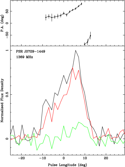
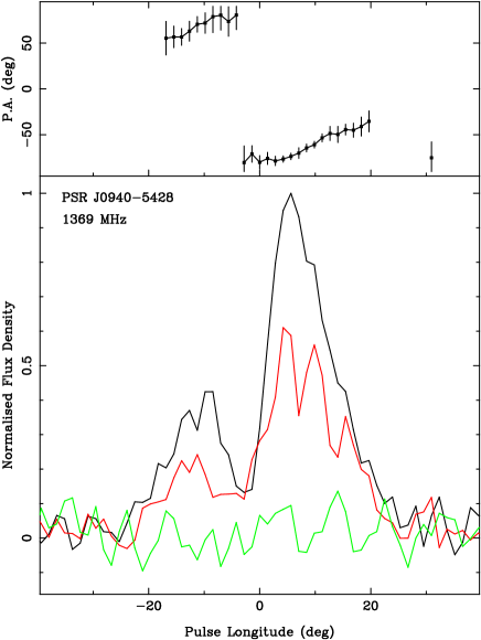
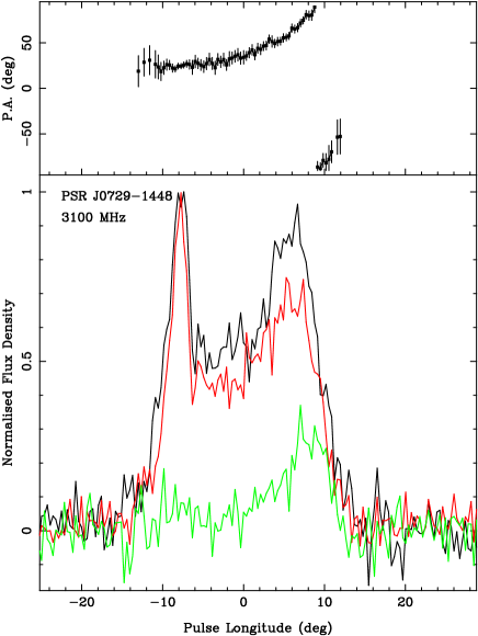
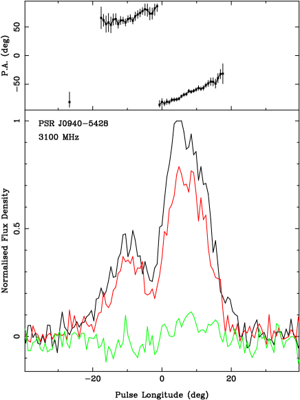
Figure 1: Polarization profiles at 1.4 GHz and 3.1 GHz for PSRs J0729$-$1449 and J0940$-$5428. The top panel of each plot shows the PA variation with respect to celestial north as a function of longitude. The PAs are corrected for RM and represent the (frequency independent) value at the pulsar. The lower panel shows the integrated profile in total intensity (thick line), linear polarization (dark grey line) and circular polarization (light grey line). The choice of longitude zero for each pulsar at the symmetrical midpoint of the profile and the profiles at the two frequencies have been aligned as closely as possible.

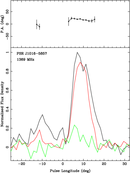
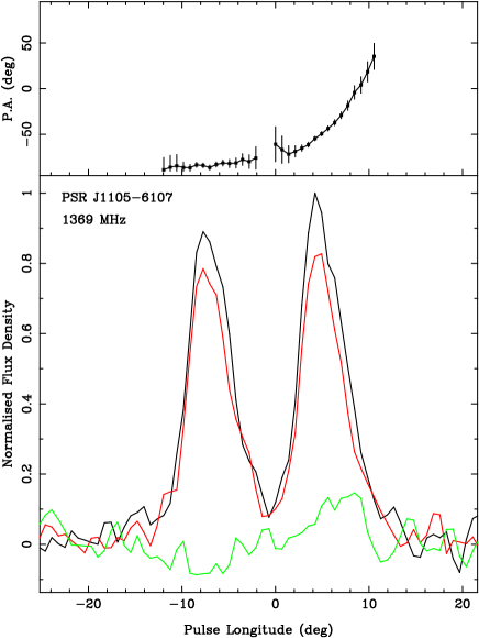
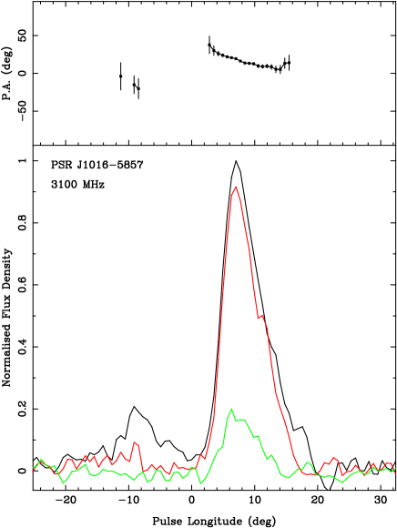
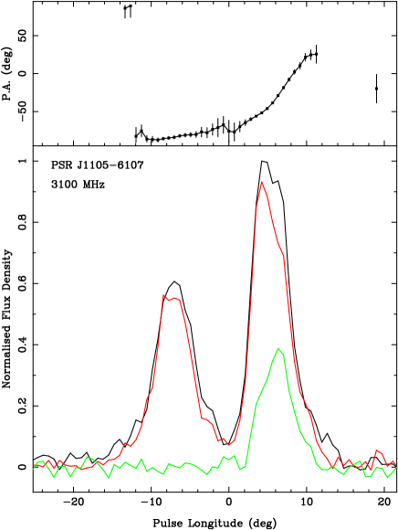
Figure 2: Polarization profiles at 1.4 GHz and 3.1 GHz for PSRs J1016$-$5857 and J1105$-$6107. See Fig 1 for details.

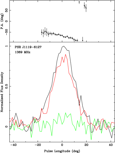
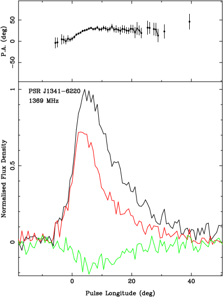
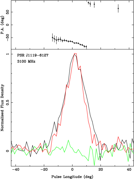
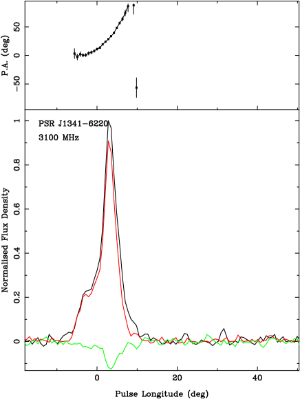
Figure 3: Polarization profiles at 1.4 GHz and 3.1 GHz for PSRs J1119$-$6127 and J1341$-$6220. See Fig 1 for details.

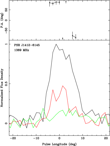
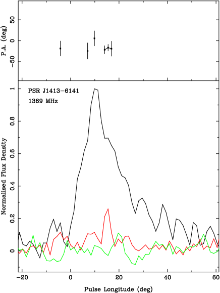
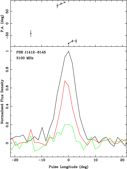
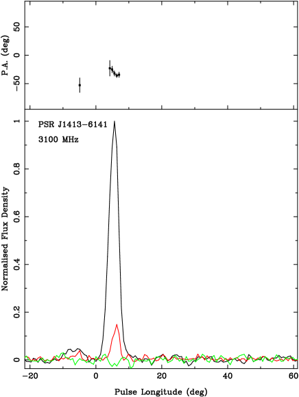
Figure 4: Polarization profiles at 1.4 GHz and 3.1 GHz for PSRs J1412$-$6145 and J1413$-$6141. See Fig 1 for details.

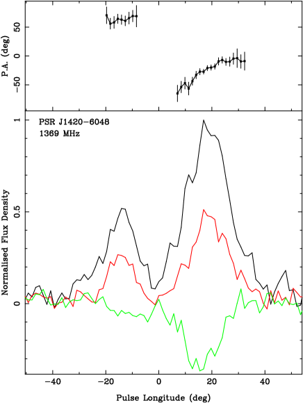
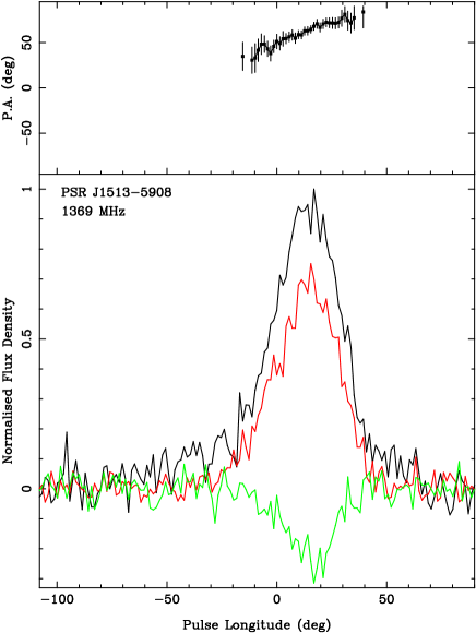
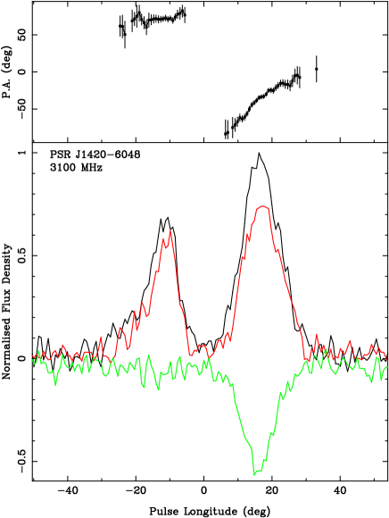
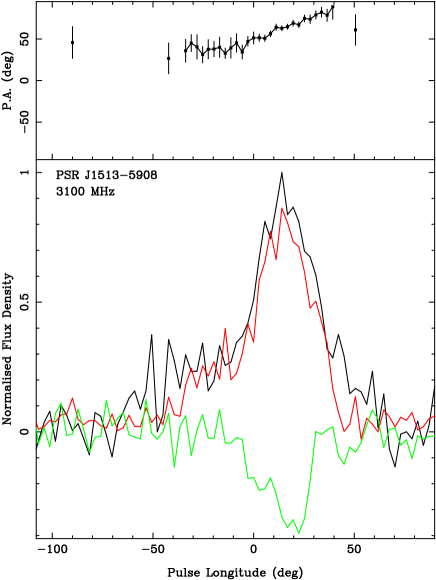
Figure 5: Polarization profiles at 1.4 GHz and 3.1 GHz for PSRs J1420$-$6048 and J1513$-$5908. See Fig 1 for details.

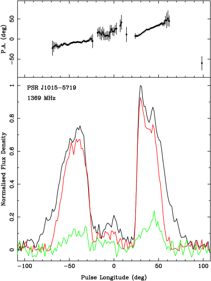
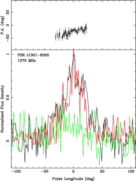
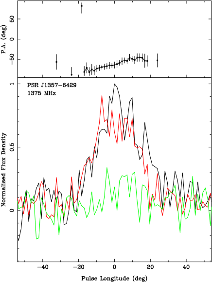
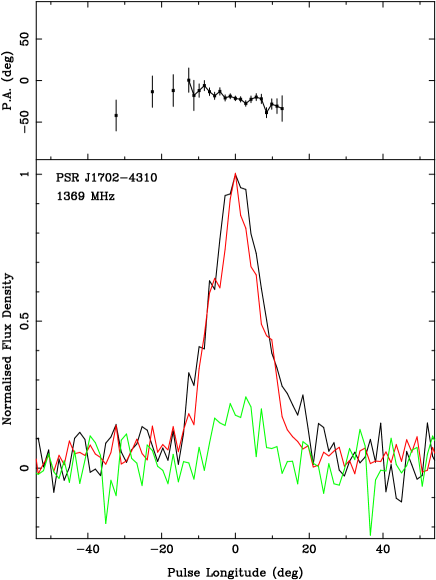
Figure 6: Polarization profiles for PSRs J1015$-$5719, J1301$-$6305, J1357$-$6429 amd J1702$-$4310 which were observed only at 1.4 GHz. See Fig 1 for details.

PSR J1015$-$5719: Observations were made only at 1.4 GHz for this pulsar. The profile is a wide double with emission over nearly 200 degrees of longitude. A small central component is also visible. It is interesting that the steep edges of the profile appear on the interior rather than the exterior of the components. This is the opposite to what is generally observed. Circular polarization is present against both the leading and trailing component. The linear polarization is similar against both components; it is very high except for the wings of the pulse where it is virtually zero. This implies that both components must themselves be composed of several individual components. We will return to this point later. It appears likely that there is an orthogonal jump between the central and trailing components.

PSR J1016$-$5857: Similar to PSR J0940$-$5428, the profile shows two components of which the trailing component is dominant. The polarization is low in the leading component but relatively high in the trailing component, as is the circular polarization. The behaviour of the PA across the leading component is unclear. Across the trailing component, the PA seems rather flat at 1.4 GHz but appears to have significant negative slope at 3.1 GHz. The profile is wider at the lower freqeuency.

PSR J1105$-$6107: The profile at 1.4 GHz is similar to that seen in Crawford et al. (2001) except that our better time resolution clearly splits the two components. The pulse profile consists of two components, nearly equal in strength at 1.4 GHz but with the trailing component dominant at 3.1 GHz. The linear polarization is high throughout but circular polarization is only present under the trailing component. The PA swing is flat under the leading component and steepens under the trailing component.

PSR J1119$-$6127: The pulse profile is a similar quasi-Gaussian shape at both frequencies although the 3.1 GHz profile is slightly narrower than its 1.4 GHz counterpart. The percentage linear polarization is high throughout the profie and the PA swing is flat.

Table 2: Constraints on geometric angles and emission heights from RVM fits

Jname	Bname	rlc	$\alpha$	$|\beta|$	$\phi_{0}$	PA0	hem	$h_{\rm em}/r_{\rm lc}$	$\rho_{o}$
		(km)	(deg)	(deg)	(deg)	(deg)	(km)		(deg)
J0729$-$1448		12000	–	$<$9	10.3	$-$82.2	630	0.053	20
J0940$-$5048		4200	–	$<$20	2.8	$-$85.4	60	0.015	11
J1015$-$5719		6700	101$\pm$5	20$\pm$5	12.9	62	380	0.057	21
J1105$-$6107		3000	–	$<$4	8.5	$-$2.2	110	0.037	16
J1119$-$6127		19500	–	$<$20	25.9	–	2200	0.11	29
J1341$-$6220	B1338$-$62	9200	–	$<$5	6.9	72.5	280	0.031	15
J1420$-$6048		3300	–	$<$15	12.3	$-$61.0	175	0.053	20
J1513$-$5908	B1509$-$58	7200	–	–	14.8	63.0	465	0.064	22

PSR J1301$-$6305: The profile consists of a single component which occupies about 100 degrees of longitude. It is highly polarized and shows a shallow swing of position angle across the pulse. It most resembles the profile of PSR J1513$-$5908 described in more detail below. The pulsar was observed only at 1.4 GHz.

PSR J1341$-$6220 (B1338$-$62): The profile at 1.4 GHz is similar to that published in Crawford et al. (2001). It is largely dominated by the scattering tail (hence the large apparent width) though there is a hint of an initial leading component. At 3.1 GHz the scattering is significantly reduced and the emerging leading component can clearly be seen. The pulsar has very high linear polarization and some circular polarization under the main component. The PA swing is initially flat before rising steeply against the trailing component.

PSR J1357$-$6429: The profile shows a single component with high linear polarization and a shallow swing of position angle. There are no observations at the higher frequency for this pulsar.

PSR J1412$-$6145: The profile at 3.1 GHz is significantly narrower than that at 1.4 GHz and the linear polarization is also higher at the higher frequency. It seems likely that the trailing edge of the lower frequency profile contains an unpolarized component which is not present at the higher frequency.

PSR J1413$-$6141: The pulse profile at 1.4 GHz seems to consist of a small leading component followed by a dominant second component which is scatter broadened. At 3.1 GHz the higher signal to noise allows the leading component to be seen more clearly. The dominant component has some linear polarization but virtually no circular polarization and a steep PA swing across it. The profile appears very narrow at 3.1 GHz, however, the initial leading component is below the 10 per cent intensity level and would add another 15° to the width. This is the only pulsar in the sample in which the linear polarization is low. The derived value for the RM is necessarily uncertain.

PSR J1420$-$6048: The pulse profile at 1.4 GHz is similar to that presented in Roberts et al (2001). There are two components, both highly linearly polarized with significant circular polarization only under the trailing component. The PA is flat under the leading component but rises steeply under the trailing component. At 3.1 GHz the leading component is slightly stronger relative to the trailing component than at 1.4 GHz and overall the profile is narrower perhaps due to scattering at the lower frequency.

PSR J1513$-$5908 (B1509$-$58): The profile has a high degree of linear polarization and a significant amount of circular polarization at both 1.4 and 3.1 GHz. In our data we see a hint of a leading component at 1.4 GHz which has become readily apparent at 3.1 GHz. The PA swing is initially flat before steepening under the trailing component. The pulsar appears to be more highly linearly polarized at 3.1 GHz than at 1.4 GHz. The width has also increased at 3.1 GHz because of the emergence of the leading component. The polarization profile at 1.4 GHz is similar to that in Crawford et al. (2001) although we note that our polarization fraction is somewhat lower than shown by those authors.

PSR J1702$-$4310: The pulsar has a single pulse component with a width of $\sim$35°. It is highly linearly polarized and has significant circular polarization. As is typical of these single-type pulsars, the PA swing is unbroken and rather flat.

5 Fitting the RVM

We have attempted to fit the rotating vector model (RVM) to the position angle swing for each pulsar in our sample. As is usual, $\alpha$ is poorly constrained in all cases (except for PSR J1015$-$5719), whereas a constraint can be placed on $\beta$ for about half the sample. However, the location of $\phi_{0}$ can often be located with good precision (at least in a statistical sense). The results are the same within the errors at both 1.4 and 3.1 GHz for those pulsars with dual frequency observations. The only exception to this is PSR J1341$-$6220 which is highly scattered at the lower frequency and for which we did not attempt a fit. Table 2 lists the pulsars from which meaningful constraints were obtained from the fitting. The third column gives the light cylinder radius of the pulsar, columns 4 and 5 give the geometrical angles. Column 6 gives $\phi_{0}$, the location of the inflexion point of the PA curve relative to the zero point of longitude taken from Figures 1-6.

PSR J1015$-$5719 is the only pulsar in the sample which provides a good RVM fit with strong constraints on the geometric angles. This is because the width of the profile is large and the presence of the central component means that PA values can be obtained almost throughout the entire longitude range. Even in this case, however, there are two possible RVM fits that can be made. The best fit is obtained only after adding an orthogonal jump between the central and trailing component. Figure 7 shows the $\chi^{2}$ contours in the $\alpha$-$\beta$ plane in the left hand panel, with the right hand panel showing the data and the best fit to the PA with $\alpha=101\degr,\beta=-20\degr$. The addition of the orthogonal jump ‘forces’ $\phi_{0}$ to be $\sim$13°. If the orthogonal jump is omitted, an RVM fit yields $\alpha\sim 86\degr,\beta\sim-10\degr$ and the best fit line passes underneath the majority of the central component PA values. In this case, $\phi_{0}$ lies at a longitude of $\sim$250°, significantly after the emission locations. Whichever fit is chosen, small values of $\alpha$ are ruled out and the pulsar appears to be an orthogonal rotator viewed at a rather large impact angle. Note that the $\alpha$ and $\beta$ values quoted here are corrected for the ‘PA convention problem’ [Everett & Weisberg 2001], wherein observed PAs increase counter-clockwise while the RVM model assumes the opposite convention.

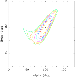
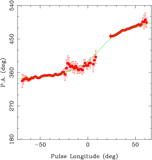
Figure 7: RVM fitting to PA swing in PSR J1015$-$5719. The left hand panel shows the $\chi^{2}$ contours in the $\alpha$-$\beta$ plane. The right hand panel shows the data (with the addition of an orthogonal jump at longitude $\sim$15°, cf Fig. 6) and the best fit with $\alpha$=101°, $\beta$=$-$20°.

For PSR J1119$-$6127, we get similar results to Crawford & Keim (2003) in that $\beta$ must be less than about 20°, and $\alpha$ is almost unconstrained. As they do, we also derive $\phi_{0}$ to be on the far trailing edge of the pulse profile. Although there is no linear polarization at this location we can estimate PA₀ to be $\sim$33°from the RVM fit. For PSR J1420$-$6048, we find that $\alpha$ and $\beta$ cannot be as well constrained as claimed by Roberts et al. (2001) who derived $\alpha<35\degr$ and $\beta\sim 0.5\degr$. For PSR J1513$-$5908, contrary to Crawford et al. (2001), we cannot constrain $\alpha$, and we therefore cannot exclude the estimate of 60° made by Romani & Yadigaroglu (1995) from the high energy pulse profile. Interpretation of the X-ray morphology of the pulsar wind nebula yields evidence that $\alpha+\beta$ is greater then 70°[Brazier & Becker 1997, Yatsu et al. 2005]. If this value is correct, our fit then constrains $\alpha$ to lie between 30° and 150°.

6 Polarization of young pulsars

It is evident even from a cursory glance at Figs 1$-$6 that many of the profiles of these young pulsars have remarkably similar characteristics. First, we see that these pulse profiles are relatively simple, unlike the highly complex profiles seen in older pulsars (as already pointed out decades ago by Huguenin et al. 1971). Lyne & Manchester (1988) concluded that this was because the relative spectral index of core and cone component was age dependent. Of the 14 pulsars studied, 9 are double profiled with the trailing component dominating in all cases. Some have almost equal amplitude components (e.g. PSR J1420$-$6048) but in others the ratio is rather large (e.g. PSR J1513$-$5908). Seven of the 9 which have measurable circular polarization have so only under the trailing component. All 9 show a flat PA swing followed by a steeper swing under the trailing component. The five pulsars which do not have multi-component profiles are PSRs J1119$-$6127, J1301$-$6305, J1357$-$6492, J1412$-$6145 and J1702$-$4310. These have single components and a rather flat PA swing with little or no circular polarization. Finally, 12 of the 14 have large degrees of linear polarization (in excess of 50 per cent) and no obvious orthogonal mode jumps in the profiles with the exception being PSR J1015$-$5719 and possibly PSR J1413$-$6141. The spectral index evolution between these two frequencies shows no obvious trends in the 8 pulsars with two components and dual frequency measurements. Three show a flatter index leading component, three have a flatter index trailing component and the remaining two have similar indicies for both leading and trailing components!

We note that these features are not only seen in the present data but also in previous polarization observations of young pulsars [Qiao et al. 1995, von Hoensbroech, Kijak & Krawczyk 1998, Crawford, Manchester & Kaspi 2001, Karastergiou, Johnston & Manchester 2005]. Nearly all have high linear polarization and those pulsars with two components have the trailing component dominant (e.g. PSRs B1610$-$50, B1643$-$43, B1758$-$23, B1800$-$21, B1823$-$13). The only exception to this rule is the Vela pulsar in which the leading component dominates the profile below 5 GHz.

There are two possible explanations for the morphology of these young pulsars. In the first scenario, the two observed components represent the leading edge of a cone and a more central component, with the trailing edge entirely absent. In this case, one expects an asymmetric PA swing (as seen) and also increased circular polarization under the central component (as also seen). Generally, however, conal components have a flatter spectral index than core components and under this picture one might expect the leading component to dominate at higher frequencies (since conal components tend to dominate over core components at high frequencies) and this is not obviously the case. However, observations over a wider frequency range (especially very low frequencies) might help solve this puzzle. One also has to explain why the trailing edge is entirely absent in these pulse profiles, but this follows the trend noted by Lyne & Manchester (1988) that leading edge cones dominate over trailing edge.

The second possibility is that the two principal observed components mark ‘classical’ double emission with the magnetic pole crossing near the symmetrical centre of the pulse profile. In this case, the asymmetry of the PA swing is then due to A/R which has a greater effect in rapidly spinning pulsars than in slowly spinning ones. The question arises as to why the trailing component always dominates and has significant circular polarization. The single component pulsars would then either be an extreme case where the leading component is absent and only the trailing component is present, or a grazing cut through the outer edge of the emission cone. The latter seems more plausible in light of the flat PA swings seen in the single component pulsars. This explanation goes against the trend shown by Lyne & Manchester (1988) where, in pulsar with partial cones, generally the leading component dominates. Taking all the data on young pulsars into account, we also violate the correlation (in 9 out of 15 cases) between the handedness of circular polarization and the sense of PA swing in conal pulsars found by Han et al. (1998). On balance however, we favour this possibility for a number of reasons. First that PSR J1015$-$5719 clearly shows a component between the two main components. Secondly, both components generally have the same width, and the symmetry point lies between the components. Finally, conal components generally have flat spectral indices as do young pulsars in general.

6.1 Emission Heights

If we assume the latter interpretation is the correct one, then we can use the results of the RVM fitting to derive the emission height of the radiation. We do this by first deriving the longitude of the midpoint of the pulsar profile using its inherent symmetry, which we denote $\phi_{s}$. Note that in Figures 1$-$6 we have located $\phi_{s}$ at zero longitude as far as possible. Then, we use the value of $\phi_{0}$ given in Table 2 to obtain the emission height by computing $\delta\phi({\rm PA})=\phi_{0}-\phi_{s}$ and attributing the difference to the effects of A/R. Application of equation 2 then leads to a determination of the emission height. These heights are listed in column 8 of Table 2; column 9 lists the heights in terms of the fraction of the light cylinder radius. From the emission heights we can compute the cone half-opening angle at the last open field line, $\rho_{o}$, via equation 4. These values are shown in column 10 of Table 2. The values of $\rho_{o}$ are distributed between 10 and 30 degrees.

The results show that the emission height for all these pulsars lies between 5 and 15 per cent of the light cylinder. This is significantly higher than the 1-2 per cent heights found for older pulsars [Gupta & Gangadhara 2003]. We caution however against interpreting these values too literally. In recent years evidence has built up that the emission height at a given frequency is not constant across the beam but is higher at the edges of the cone and lower in the middle [Gupta & Gangadhara 2003]. If this is the case, A/R affects the core and cone by different amounts and the symmetrical midpoint of the profile will not necessarily correspond to the core location and the emission heights computed through A/R will be underestimates. Finally, other effects such as refraction effects [Petrova 2000] and magnetic field sweepback can distort this picture still further [Arendt & Eilek 1998, Dyks & Harding 2004].

We note there is a strong inconsistency in the interpretation of the data on PSR J1015$-$5719. The RVM fit shows the pulsar is nearly an orthogonal rotator; if this is the case then the very large pulse width naturally implies the emission must come from high in the magnetosphere. On the other hand, the value of the emission height derived from the location of $\phi_{0}$ is rather small. There are two possible sources of error or confusion. The RVM fit might be incorrect and the pulsar is really an aligned, rather than orthogonal rotator. This is possible, witness for example the continuing discussion on whether PSR B0950+08 is aligned or orthogonal [Everett & Weisberg 2001], but seems unlikely given the goodness of fit. Secondly, assigning the offset in $\phi_{0}$ as arising due to A/R is in error due to the reasons we suggested above.

However, there exists a further appealing solution for PSR J1015$-$5719. This comes from recognising that the measured A/R yields the emission height of the core emission and may not reflect the emission height of the conal emission if this occurs significantly higher in the magnetosphere than the core emission [Gupta & Gangadhara 2003]. To test this, we have therefore decomposed the profile of PSR J1015$-$5719 into 7 Gaussians, 3 for the leading edge, a central component and 3 for the trailing edge. The location of the centroid of these Gaussians occurs at longitudes $-$72°, $-$52°, $-$36°, 0°, 31°, 44° and 56°(cf Figure 6). Immediately one can see that the locations are asymmetric, with the trailing components closer to the core component than the leading components, exactly as expected in the picture of Gangadhara & Gupta (2001). We can use this asymmetry, in conjunction with the derived emission height of $\sim$400 km for the core component to derive the heights of the 3 conal components (see equation 5). These are (from inner to outer) 550 km, 650 km and 850 km respectively. Using the more exact formalism of Gangadhara (2005) which takes into account the geometrical angles the height of the outermost cone increases to 925 km. This helps solves the problem of having an orthogonal rotator with a seemingly small emission height and a wide profile. Indeed the emission height of the core is small, but the outer cones are at a significantly higher height, yielding a wide profile.

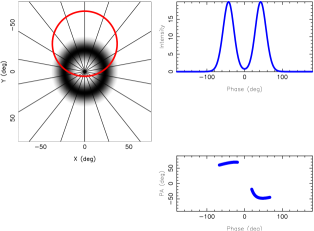
Figure 8: Simulation of a pulse profile and PA swing from our simple model. Parameters are $\alpha$=30°, $\beta$=5°, and we assume a pulse period of 100 ms with an emission height of 250 km. The left panel shows the emission pattern with the line of sight traverse superposed. The top right panel shows the resultant pulse profile with the bottom right panel showing the PA swing, which is delayed relative to the total intensity profile by an amount consistent with the emission height and the effects of A/R.

6.2 A Generic Young Pulsar Beam Model

We have concluded that young pulsar beams generally consist of a hollow cone, with little or no emission from the center. The double profiles arise from cuts close to the magnetic pole, the single profiles are grazing trajectories along the cone. We quantify this by adopting a canonical young pulsar with a spin period of 0.1 s. The light cylinder radius is at $\sim$5000 km with the emission zone located at $\sim$250 km, consistent with the results in Table 2. These parameters naturally lead to a beam half-opening angle of $\sim$20°. A simple beam model can then be created in which $\rho$=20° and there is a single hollow cone of emission located at the beam edge. The conal emission zone is relatively wide, has a Gaussian amplitude distribution and takes up $\sim$0.2 of the beam. There is no core emission. We then choose random values of $\alpha$ and $\beta$ and compute the line of sight relative to the beam in order to produce a simulated pulse profile. At the same time, we can construct a PA swing based on the geometric angles, assuming the RVM is correct. The PA swing is then delayed in longitude with respect to the profile by an amount consistent with the emission heights and the effects of A/R. Fig 8 shows an example. We find from the simulations that $\sim$50 per cent of pulsars are potentially detectable (i.e. we have some sightline across the open field lines); of these $\sim$45 per cent have double profiles and $\sim$55 per cent have single profiles. Most of the double component pulsars have widths of $\sim$40°, with a small minority having much wider beams. For the single components, there is a ratio of 2:1 between narrow and wide profiles. The results from this simple simulation are very similar to the observed results. In the observed sample, there is roughly an equal split between profiles with single components and those with two components. Most of the double component profiles have similar widths, with the occasional wide double. In contrast the single component pulsars show a larger variety in pulse widths as seen in the simulation.

7 Derived proper motion directions and their implications

As discussed in the introduction, we can potentially determine the direction of motion of the pulsars through knowledge of the position angle of the rotation axis under the assumption that they are aligned with the velocity direction. Johnston et al. (2005) pointed out that, even if the vectors are aligned, the polarization PA at $\phi_{0}$ could be perpendicular to the rotation axis if the pulsar emits in the orthogonal mode. We have seen from the discussion of the pulse profiles, it is very difficult to correctly assess the longitude of the magnetic pole in these young pulsars. We can only really be confident in the cases where the RVM fit returns an accurate value of $\phi$ and hence PA₀ as listed in Table 2 above. This is only the case for 7 pulsars in our sample, and one of these (PSR J1119$-$6127) has no polarization at the location of $\phi_{0}$. We describe the other six pulsars here. The value of PA₀ has an inherent 180° ambiguity because of the definition of position angle of linear polarization. Also, it is possible that PA₀ can be 90° different from the true value of the rotation axis position angle, if the pulsar is emitting in the orthogonal mode (for full details see Johnston et al. 2005). Hence in what follows, we assume that either PA₀ or PA${}_{0}\pm 90\degr$ will be parallel to the velocity vector of the pulsar. This implicitly assumes that velocity vector is aligned with the rotation axis as found by Johnston et al. (2005) but we caution that this might not be a general rule.

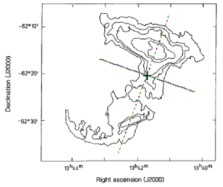
Figure 9: Radio continuum image of SNR G308.8$-$0.1 (Caswell et al. 1992). The plus marks the position of PSR J1341$-$6220. The solid line denotes PA₀ from our measurements. The dashed line is orthogonal to PA₀ and is our preferred proper motion direction.

PSRs J0729$-$1448 and J0940$-$5048: These two pulsars have no apparent associations with high energy emission or SNRs. The value of PA₀ and hence the direction of the rotation axis is parallel or perpendicular to $-$82.2 and $-$85.4 degrees respectively.

PSR J1105$-$6107: In this pulsar, we showed in Section 2 that one might expect the velocity vector to point at 135° if the pulsar was associated with SNR G290.1$-$0.8. The value of PA₀ that we derive from the RVM fit, $-$2.2°, would then seem to imply that the pulsar did not originate from SNR G290.1$-$0.8. The pulsar has a relatively large characteristic age and it may be that its parent SNR has simply dissipated.

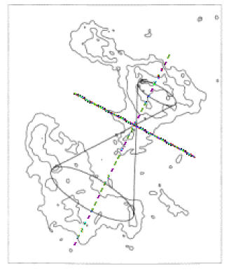
Figure 10: Radio continuum image of SNR G320.4$-$1.2. PSR J1513$-$5908 lies at the intersection of the two cones which represent a possible outflow geometry based on the continuum morphology (Gaensler et al. 1999). The solid line denotes PA₀ from our measurements. The dashed line is orthogonal to PA₀ and is our preferred proper motion direction.

PSR J1341$-$6220: The main axis of symmetry of the peculiar SNR in which PSR J1341$-$6220 is embedded has a position angle of $-$20°, which is $\sim$90° offset from our measured PA₀ of 72.5°. It seems likely therefore that the pulsar is moving along this symmetry axis, the rotation axis also points in this direction and it emits in the orthogonal mode. Figure 9 shows the SNR/PSR association with our derived value of PA₀ and the preferred proper motion direction.

PSR J1420$-$6048: The pulsar lies in a highly complex region of the Galactic plane as detailed above. A proper motion in virtually any direction would intersect something of interest! It so happens that the perpendicular to our PA₀ of $-$61° points at the centre of the ‘Kookaburra’ complex. Is PSR J1420$-$6048 a pulsar moving at $\sim$400 km s^-1 which originated in the centre of the ‘Kookaburra’, punctured through the shell and is currently creating a wind bubble similar to the picture seen in the ‘Duck’ system [Gaensler & Frail 2000, Thorsett, Brisken & Goss 2002]?

PSR J1513$-$5908: The PA of the symmetry axis of the PWN in which the pulsar is embedded is 150°$\pm$5°. Gaensler et al. (2002) infer that the rotation axis of the pulsar must also have this PA to conform with their model. Our polarization measurements yield PA₀ of 63°, which differs by 87° from the Gaensler et al. (2002) conjecture. We therefore support the idea that the PWN symmetry axis is indeed aligned with the pulsar’s rotation axis and that the pulsar emits in the orthogonal mode as in the Vela pulsar (Johnston et al. 2005) and the above case of PSR J1341$-$6220. If the correlation between the spin axis and the velocity vector in pulsars is also correct then we predict the pulsar’s proper motion will also lie along this axis. Figure 10 shows the SNR/PSR association with our derived value of PA₀ and our proposed proper motion direction.

8 Conclusions

We have observed 14 young pulsars and obtained calibrated polarization profiles. The profiles of young pulsars are generally simple and fall into two categories. In the first, the profiles consist of two, highly polarized components with a flat PA swing across the first component and a steep swing across the second. The second component is nearly always brighter than the first component. The correlation pointed out by Han et al. (1998) between the sign of circular polarization and the sense of swing of the PA appears not to apply in these double pulsars. The second category consists of a simple, broad single component with high polarization and a shallow swing of position angle.

We interpret these results as showing that the emission beams of young pulsars consist simply of a single emission cone located near the last open field lines. Core emission is absent or rather weak. Emission arises between 1 and 10 percent of the light cylinder radius which is significantly higher than the emission zone in older pulsars. This simple model explains many of the features of the observations. Two questions remain: why are the trailing components always brighter and why do they generally have more circular polarization?

We predict that PSRs J1341$-$6220 and J1513$-$5908 have aligned rotation and velocity axes and it would be useful to measure the proper motion of these pulsars as verification.

References

- [Arendt & Eilek 1998] Arendt P. N., Eilek J. A., 1998, ApJ, Submitted
- [Bilitza 2003] Bilitza D., 2003, Advances in Space Research, 31, 757
- [Blaskiewicz, Cordes & Wasserman 1991] Blaskiewicz M., Cordes J. M., Wasserman I., 1991, ApJ, 370, 643
- [Brazier & Becker 1997] Brazier K. T. S., Becker W., 1997, MNRAS, 284, 335
- [Camilo et al. 2000] Camilo F., Kaspi V. M., Lyne A. G., Manchester R. N., Bell J. F., D’Amico N., McKay N. P. F., Crawford F., 2000, ApJ, 541, 367
- [Camilo et al. 2001] Camilo F. et al., 2001, ApJ, 557, L51
- [Case & Bhattacharya 1999] Case G., Bhattacharya D., 1999, ApJ, 521, 246
- [Caswell et al. 1992] Caswell J. L., Kesteven M. J., Stewart R. T., Milne D. K., Haynes R. H., 1992, ApJ, 399, L151
- [Crawford & Keim 2003] Crawford F., Keim N. C., 2003, ApJ, 590, 1020
- [Crawford, Manchester & Kaspi 2001] Crawford F., Manchester R. N., Kaspi V. M., 2001, AJ, 122, 2001
- [Crawford et al. 2001] Crawford F., Gaensler B. M., Kaspi V. M., Manchester R. N., Camilo F., Lyne A. G., Pivovaroff M. J., 2001, ApJ, 554, 152
- [D’Amico et al. 2001] D’Amico N. et al., 2001, ApJ, 552, L45
- [Doherty et al. 2003] Doherty M., Johnston S., Green A. J., Roberts M. S. E., Romani R. W., Gaensler B. M., Crawford F., 2003, MNRAS, 339, 1048
- [Dyks & Harding 2004] Dyks J., Harding A. K., 2004, ApJ, 614, 869