Theoretical light curves for deflagration models of Type Ia supernova

Abstract

Aims. We present synthetic bolometric and broad-band $UBVRI$ light curves of SNe Ia, for four selected 3-D deflagration models of thermonuclear supernovae.

Methods. The light curves are computed with the 1-D hydro code stella, which models (multi-group time-dependent) non-equilibrium radiative transfer inside SN ejecta. Angle-averaged results from 3-D hydrodynamical explosion simulations with the composition determined in a nucleosynthetic postprocessing step served as the input to the radiative transfer model.

Results. The predicted model $UBV$ light curves do agree reasonably well with the observed ones for SNe Ia in the range of low to normal luminosities, although the underlying hydrodynamical explosion models produced only a modest amount of radioactive ⁵⁶Ni (i.e. $\sim$ 0.24 - 0.42 M_☉) and relatively low kinetic energy in the explosion (less than $0.7\times 10^{51}$ erg). The evolution of predicted $B$ and $V$ fluxes in the model with a ⁵⁶Ni mass of 0.42 M_☉ follows the observed decline rate after the maximum very well, although the behavior of fluxes in other filters somewhat deviates from observations, and the bolometric decline rate is a bit slow. The material velocity at the photospheric level is of the order of $10^{4}$ km s^-1 for all models. Using our models, we check the validity of Arnett’s rule, relating the peak luminosity to the power of the deposited radioactive heating, and we also check the accuracy of the procedure for extracting the ⁵⁶Ni mass from the observed light curves.

Conclusions. We find that the comparison between theoretical light curves and observations provides a useful tool to validate SN Ia models. The steps necessary to improve the agreement between theory and observations are set out.

1 Introduction

With three-dimensional simulations (e.g. Hillebrandt et al., 2000; Reinecke et al., 2002; Gamezo et al., 2003; Röpke & Hillebrandt, 2005b), type Ia supernova (hereafter SN Ia) explosions can be modeled self-consistently. Such models are constructed from first principles, avoiding free parameters in the description of physical processes. The only parameters entering are the initial state of the exploding white dwarf star and the configuration of flame ignition, which must be determined in separate studies of progenitor evolution.

Consequently, the important question is to what degree do these models describe real SNe Ia explosions. This can only be answered through comparison with observations of nearby events (e.g. Pignata et al. 2004; Benetti et al. 2004; Stehle et al. 2005). To this end, observables need to be derived from theoretical explosion models. In this paper, we show how synthetic light curves (both bolometric and broad-band UBVRI) can be obtained from a set of three-dimensional deflagration models of SN Ia explosions (Travaglio et al. 2004; Röpke et al. 2005; Röpke & Hillebrandt 2005b). We emphasize that the present study is intended to demonstrate the derivation of light curves from theoretical models and to analyze the use of these as a tool to validate such models. Therefore the chosen models do not reflect particularly realistic simulations and have known weaknesses. Judging the validity of explosion models in terms of derived observables requires more elaborate models and this issue will be addressed in a forthcoming publication.

When one succeeds in constructing SN Ia explosion models that are consistent with observations, they will be used to tackle questions concerning the application of SNe Ia in determining cosmological parameters. Since these objects need to be calibrated on the basis of empirical recipes to serve as distance indicators, such distance measurements are subject to uncertainty. This may be lessened by a theoretical understanding of the origin of the diversity in observables and of the calibration techniques.

The calibration methods currently applied in SN Ia cosmology are based on an empirical correlation between the blue-band magnitude of the supernova and the decline rate of its light curve (e.g. Pskovskii, 1977; Phillips, 1993; Phillips et al., 1999). As pointed out by many authors (e.g. Höflich et al., 1998; Sorokina et al., 2000; Mannucci et al., 2005), the luminosity–decline rate relation for SNe Ia is derived at low redshifts $z$, and it is unclear how it should change at high redshifts. Systematic differences of the order of $\sim$$0.1$ magnitudes (Höflich et al., 2000; Nomoto et al., 2003) can be important in cosmological applications. A sound understanding of the physical mechanism of SNe Ia is crucial in any project investigating possible systematic trends in their properties. Additionally, a radiative transfer algorithm is required to reliably relate the hydrodynamical model of the explosion to observed fluxes and spectra of SNe Ia.

Röpke & Hillebrandt (2004) and Röpke et al. (2005) have presented systematic studies of effects resulting from variations in the progenitor white dwarf’s carbon-to-oxygen ratio, its central density at ignition and its metallicity on 3-D deflagration explosion models. These were based on simple and thus only weakly exploding models and therefore such studies need to be extended with more elaborate simulations. The missing link to SN Ia cosmology in such approaches is the derivation of synthetic light curves.

This paper presents synthetic light curves for two models from the set described by Röpke et al. (2005) and for two additional 3-D models (from Travaglio et al., 2004; Röpke, 2005). We compute bolometric and broad-band $UBVRI$ light curves of SNe Ia, employing the radiation hydro code stella which simulates multi-group time-dependent non-equilibrium radiative transfer inside SN ejecta in a spherically-symmetric approximation.

First, we briefly outline the assumptions made in modeling the radiative transfer (Sec. 2). In Sec. 3 we describe parameters of the hydrodynamical models. Various observables predicted by the radiation code for the studied hydro models are presented in Sec. 4. The accuracy of determining the ⁵⁶Ni mass based on Arnett’s rule is demonstrated in Sec. 5.

The results are summarized and discussed in Sec. 6. We describe the necessary steps for future improvements of both hydrodynamical and radiative transfer models in Sec. 7.

2 Numerical Model for Radiative Transfer

Modeling the post-explosion stages of SNe Ia appears to be easier than that of core collapse supernovae (CCSNe). For thermonuclear supernovae the hydrodynamics is very simple: the coasting stage starts very early, there are no shocks, and the only additional heating mechanism is the decay of radioactive nuclei. A typical assumption for SNe Ia light curve modeling is to fully neglect the hydrodynamics. We discuss the validity of this assumption in Sect. 6.

However, with SNe Ia difficulties arise with the modeling of the radiative transfer. SNe Ia become almost transparent in the continuum at the age of a few weeks. This means that NLTE effects are stronger compared to CCSNe. Radiation decouples from matter within the entire SN Ia ejecta prior to maximum light (Eastman 1997; Blinnikov & Sorokina 2004). In this environment one cannot ascribe the gas temperature (nor any other temperature) to radiation since a SN Ia spectrum differs strongly from a blackbody. Instead, one has to solve a system of time-dependent transfer equations in many energy groups with an accurate prescription for the treatment of a enormous number of spectral lines. These lines are the main source of opacity in the ejecta (Baron et al. 1996a; Pinto & Eastman 2000b).

Recently, powerful codes have been developed in order to address the full 3-D time-dependent problem of SN Ia radiative transfer (Höflich 2002; Lucy 2005). Yet there are some basic questions, like averaging the line opacity in an expanding media, that remain controversial.

We compute broad-band $UBVRI$ and bolometric light curves of SNe Ia with the multi-energy radiation hydro code stella (Blinnikov et al. 1998; Blinnikov & Sorokina 2000). The 3-D hydrodynamic models are angle-averaged and used as input for the radiation hydro code. Time-dependent equations for the angular moments of intensity in fixed frequency bins are coupled to the Lagrangian hydro equations and solved implicitly. Therefore there is no need to ascribe any temperature to the radiation; the photon energy distribution may be quite arbitrary.

There are millions of spectral lines that lead to the formation of a SN Ia spectrum, and it is not a trivial problem to find a convenient way to treat them even in the static case. The expansion makes the problem much more difficult to solve as hundreds to even thousands of lines give their input into emission and absorption at each frequency.

The effect of line opacity is treated in the current work as an expansion opacity according to Eastman & Pinto (1993). The line list is limited to $\sim$160 thousand entries, selected from the strongest down to the weakest lines until the saturation in the expression for expansion flux opacity is achieved. The effect of extending the line list deserves further investigation, and work in this direction is underway.

The ionization and atomic level populations are described by Saha-Boltzmann expressions. However, the source function is not in complete LTE.

The source function at wavelength $\lambda$ is

$$S_{\lambda}=\epsilon_{\rm th}\,B_{\lambda}+(1-\epsilon_{\rm th})\,J_{\lambda},$$ (1)

where $\epsilon_{\rm th}$ is the thermalization parameter, $B_{\lambda}$ is the Planck function, and $J_{\lambda}$ is the angle mean intensity. In a pure LTE approximation $\epsilon_{\rm th}=1$, and in a “pure scattering” treatment $\epsilon_{\rm th}=0$. Baron et al. (1996b) compared the results of a full NLTE treatment, a pure LTE treatment, and a pure scattering treatment of the lines (in their case $S_{\lambda}$ described the source function only in a line). They found that the pure LTE case (for lines) reproduces the overall spectral shape of the NLTE case rather well, while the pure scattering case does not. In the NLTE case, the collisions within multiplets create a pseudo-thermal pool of photons which are in equilibrium among themselves.

In our code, we have rather wide energy bins that contain hundreds of strong lines, so our $S{{}_{\lambda}}$ is a complicated average of lines and continuum for a given bin. We can ascribe an arbitrary degree of thermalization to the lines. Even if we treat all lines as pure absorbers we have an appreciable contribution of photon scattering off electrons, thus the average $\epsilon_{\rm th}\neq 1$ in a bin and $S_{\lambda}$ is not in full LTE. Therefore, we prefer to call the approximation of full thermalization in lines as ‘fully absorptive lines’. The approximation of the fully absorptive opacity in spectral lines allows us to simulate NLTE effects in a simple manner. NLTE results (Baron et al. 1996b) and the ETLA approach (Pinto & Eastman 2000b) demonstrate that fully absorptive lines give an acceptable description of the overall spectral shape and subsequent optical light curves.

A similar approach to light curve modeling with LTE opacities and a comparable number of photon energy groups is used by Höflich et al. (1998) who employed NLTE calculations (Höflich, 1995) to calibrate scattering in lines. A full NLTE time-dependent treatment is within reach and is already being implemented by other groups (Höflich 2002; Lucy 2005), but much work remains to be done before all problems are solved.

The deposition of gamma rays produced in radioactive decays of Fe-group isotopes (mostly due to ⁵⁶Ni and ⁵⁶Co) should be properly considered. After being emitted, the gamma rays travel through the ejecta and can end up either thermalized or in non-coherent scattering process. To determine which way they end up one has to solve the transfer equation for gamma rays together with hydrodynamical equations. The full system of equations should also involve the radiative transfer equations in the range from soft X rays to infrared wavelengths for the expanding medium.

We do not write down the full set of equations solved by stella (Blinnikov et al. 1998), but we point out that hydrodynamics coupled to radiation is fully computed (homologous expansion is not assumed). Since there are several different approaches found in literature, here (and in Sect. 6) we discuss in some detail the use of the matter temperature equation.

The equation for the material temperature $T$ is derived from the first law of thermodynamics,

$$de+pdV=de-{p\over\rho^{2}}\,d\rho=\left({\partial e\over\partial T}\right)_{\rho}\,dT-{T\over\rho^{2}}\,\left({\partial p\over\partial T}\right)_{\rho}\,d\rho,$$ (2)

which takes the form:

$$\biggl{(}{\partial e\over\partial T}\biggr{)}_{\rho}{\partial T\over\partial t}=\varepsilon+4\pi\int\limits_{0}^{\infty}(\alpha_{\nu}J_{\nu}-\eta_{\nu})d\nu-4\pi{\partial{(r^{2}u)}\over\partial m}T\biggl{(}{\partial p\over\partial T}\biggr{)}_{\rho}\;.$$ (3)

Here $p=p(\rho,T)$ is the material pressure, $\rho$ is the density, $m$ is the Lagrangian coordinate (i.e. the mass inside radius $r$), $J_{\nu}$ is equal to ${1\over 2}\int_{-1}^{1}d\mu\,I_{\nu}$, $e$ is the specific internal energy of matter, $\alpha_{\nu}$ is the absorption coefficient per unit mass, and $\varepsilon$ is the specific power of the local heating (here due to gamma-ray energy deposition). In the case of LTE the emission coefficient $\eta_{\nu}$ is equal to $\alpha_{\nu}B_{\nu}$.

We should note that the last equality in Eq. (2) is based on the expression $de+pdV=Tds$, where $s$ is specific entropy, i.e. not only the first, but also the second law of thermodynamics for reversible processes is used in the derivation. In other words, this relation is valid when $e$ and $p$ are functions of $\rho$ and $T$. While radiation is non-equilibrium in our approximation, ionization and atomic level populations are described by Saha-Boltzmann equations. Therefore Eqs. (2) and (3) are applicable. If ionization and excitation depend on other parameters in NLTE, and/or are described by kinetic equations, one must use other forms of the energy equation (see e.g. Sorokina et al. 2004).

Another possible approach is to extract matter energy $e$ from the equations of evolution for radiation energy $E$ and full energy $e+E$ (e.g. Höflich et al. 1993). In both cases the matter energy $e$ is found with lower accuracy than the radiation energy $E$. This is due to the subtraction of nearly equal terms; either of $e+E$ and $E$ in the latter approach or in the heating and cooling terms of Eq. (3).

To find the radioactive energy deposition $\varepsilon$ we treat the gamma-ray opacity as a pure absorptive one, and solve the gamma-ray transfer equation in a one-group approximation following Swartz et al. (1995). The effective opacity assumed is $\kappa_{\gamma}=0.05Y_{e}\;\mbox{cm}^{2}/\mbox{g}$, where $Y_{e}$ is the total electron number density over baryon density. We have checked that this effective opacity gives good agreement for the values of the deposition and broad band fluxes found by Monte-Carlo codes after the maximum light. The rise part of the light curve is not sensitive to the variation of $\kappa_{\gamma}$ when it is changed by a factor of 3. For one of the models (b30, described below) the deposition was computed in full 3D-transport by a modification of shdom code (Evans, 1998). The agreement with 1D version is within a few percent.

The heating by the decays ⁵⁶Ni $\to$ ⁵⁶Co$\to$ ⁵⁶Fe is taken into account. It is assumed that positrons, born in the decays, are trapped and deposit their kinetic energy locally, cf. Colgate et al. (1980a, b); Chang & Lingenfelter (1993); Ruiz-Lapuente (1997); Milne et al. (1997); Ruiz-Lapuente & Spruit (1998) and Jeffery (1999) on various approaches to this problem important for late stages (the ‘tail’) of SNe Ia.

To calculate SNe Ia light curves our method can use up to 200 frequency bins and up to $\sim$400 zones in mass as a Lagrangian coordinate on a modest processor.

Major recent improvements in the code stella (introduced after the paper Blinnikov et al., 1998, was published) are described in the following. The ionization of the 15 most abundant elements (from H up to Ni) is now computed for any stage, without introducing an averaged ion approximation. As previously mentioned the line list has been extended. When computing the opacity we now take into account the change in the composition of the iron peak elements in the decay chain ⁵⁶Ni $\to$ ⁵⁶Co$\to$ ⁵⁶Fe. The most important advancement is also related to the computation of the expansion opacity: instead of interpolating the opacity in tables for preselected instants of time, it is now computed for each time step in each mesh zone. Although this approach requires much more processor time than using the tables, it is more reliable when one is interested in finding fine details for models with small differences in parameters.

3 Initial models

For this study light curves are derived using four hydrodynamical explosion models. Each model possesses different characteristics that result in a variation in the computed light curves.

The explosion models are based on a pure deflagration scenario. In this case a sub-sonic thermonuclear (“deflagration”) flame is ignited near the center of a Chandrasekhar mass carbon-oxygen white dwarf. Subsequently the flame propagates outwards generating turbulence due to generic instabilities. The interaction with turbulent motions accelerates the flame propagation velocity such that nuclear burning releases a sufficient amount of energy that completely disrupts the white dwarf. For a review on SN Ia models see Hillebrandt & Niemeyer (2000).

Details concerning the numerical techniques used to implement this scenario were presented by Niemeyer & Hillebrandt (1995), Reinecke et al. (1999a, 2002a) and Röpke (2005). The main challenge is to self-consistently model the turbulent combustion which involves a wide range of scales. To this end a Large Eddy Simulation (LES) approach is applied, which directly resolves only the largest scales of the problem (i.e. scales from the radius of the white dwarf, $\sim$2000 km, down to several kilometers). To account for the effects of turbulence on unresolved scales, a sub-grid scale model is adopted (Niemeyer & Hillebrandt 1995). The flame itself is modeled as a sharp discontinuity separating the fuel from the ashes applying the level-set method (Reinecke et al., 1999a). Since such an approach does not resolve the internal flame structure, propagation due to burning has to be prescribed. This approach however does not lead to any free parameters. The theory of turbulent combustion states that in the case of burning in the so-called flamelet regime, which applies to most parts of a SN Ia explosion, the flame propagation completely decouples from the micro-physics. It is solely determined by the turbulent motions which can be derived from the adopted sub-grid scale model. We emphasize that apart from the initial conditions that are determined from the progenitor evolution, this model contains no free parameters.

Consequently, the models used to derive the light curves from vary only in the initial conditions, i.e. the composition, the central density of the white dwarf, and the manner in which the thermonuclear flame is ignited. All models were simulated on one spatial octant of the white dwarf and mirror symmetry was assumed for the other octants. Röpke & Hillebrandt (2005b) showed that this artificial symmetry constraint does not obscure the explosion mechanism. In three of the models, the flame was ignited centrally and perturbed from spherical symmetry by toroids. Contrary to this, the b30_3d_768 model of Travaglio et al. (2004) (in the following denoted as b30), assumed a multi-spot ignition scenario in which the flame was ignited in 30 small kernels per octant. Evidently, such multi-spot scenarios can lead to more vigorous explosions than centrally ignited models (Travaglio et al. 2004; Röpke et al. 2005).

Table 1: Model parameters.

model	$\rho_{c9}$	$X(^{16}\textrm{O})$	$X(^{12}\textrm{C})$	$X(^{22}\textrm{Ne})$	$Z[Z_{\sun}]$
1_3_3	$1.0$	$0.38$	$0.545$	$0.075$	$3.0$
2_2_2	$2.6$	$0.54$	$0.435$	$0.025$	$1.0$
c3_3d	$2.9$	$0.5$	$0.475$	$0.025$	$1.0$
b30	$2.9$	$0.5$	$0.475$	$0.025$	$1.0$

The initial parameters of the models are summarized in Table 1. We assumed increasing central densities in the sequence of models 1_3_3, 2_2_2 and c3_3d. Explosion models c3_3d and b30 were set up for a 50% carbon-oxygen mixture, while the carbon mass in models 2_2_2 and 1_3_3 was set to 0.46 and 0.62, respectively.

The detailed nucleosynthesis of each model was derived with a post-processing technique that uses data obtained from tracer particles in the explosion simulation (see Travaglio et al., 2004; Röpke et al., 2005, for a detailed discussion concerning this method). During the post-processing solar metallicity was assumed for all the models except 1_3_3. There an assumed three times increase metallicity of the main sequence progenitor of the white dwarf resulted in a ²²Ne mass fraction of 0.075. The ²²Ne mass fraction was included in the post-processing by lowering the ¹²C fraction.

With respect to the computational setup, model c3_3d differs from the other three models. These were calculated on a static grid with uniform fine-resolved inner parts and exponential grid spacing in the outer regions to capture at least parts of the expansion. Models b30, 2_2_2, and 1_3_3 were followed for $1.33\,\mathrm{s}$, $1.5\,\mathrm{s}$, and $2.0\,\mathrm{s}$, respectively. The light curve derivation assumes homologous expansion at the point where the hydrodynamical explosion simulation ends. This is, however, not yet reached to a high accuracy at these times. Therefore, in model c3_3d a different approach was chosen (Röpke 2005). This simulation was carried out on a uniform computational grid co-expanding with the white dwarf. In this way it was possible to follow the evolution time to 10 s after flame ignition.

All simulations (except b30) were carried out on $[256]^{3}$ grid cells to ensuring numerical convergence (Reinecke et al. 2002a; Röpke 2005). To accommodate for a reasonable number of flame ignition kernels the resolution was increased to $[756]^{3}$ cells for model b30.

The global characteristics of the explosion models are summarized in Table 2. Detailed results from the explosion simulations can be found in Travaglio et al. (2004), Röpke & Hillebrandt (2004, 2005b) and Röpke et al. (2005) All models produce rather weak explosions, lower than canonical $1$ foe ($=10^{51}$ erg), and low amounts of ⁵⁶Ni. Although they lie in the range of variability expected from observations, only model b30 comes close to the class of “Branch normals” (Branch et al. 1993).

The remapping of 3-D models to spherical 1-D geometries has been done using the same tracer particles that were used for the nucleosynthesis calculations. A grid in radial coordinates was constructed with uniform steps in radius, the outer radius being equal to the maximum radius of the 3-D model. The number of tracer particles (all of equal mass) then determined the mass of each spherical shell constructed on the grid, and the chemical composition of the particles determines the composition of the shell. The square of the particle velocities were summed up to obtain the total kinetic energy of the shell. The motion of particles is not purely radial, however, the non-radial component is not high at the end of explosion simulation. The kinetic energy of transversal motion is of the order of $0.01$ of the radial motion (since model c3_3d was followed for a longer period the transversal motion is only $\sim 3\times 10^{-4}$ of the radial motion).

We assume that even if the non-radial component will be dissipated and goes to heat, the heat will not be radiated away because during the first several hours after the explosion all zones are optically thick. After some time this heat will be returned to the kinetic energy of the expansion. The kinetic energy and the mass of each shell determines the velocity of the shell, which is ascribed to the outer radius of the mesh zone in the radiation hydro code. The radiation hydro simulation starts for all runs at time $10^{4}$ s after the ignition of the explosion. We assume that the total energy at the end of the flame simulation $E_{\rm tot}$ (kinetic plus thermal plus gravitational) goes into $E_{\rm kin}$ at $10^{4}\,\mathrm{s}$. We have renormalized the original $E_{\rm kin}$ from the tracer particles to $E_{\rm tot}$, and this value is given in the Table 2 as $E_{\rm kin}$ initial.

As an example, the chemical composition for the model 2_2_2 is shown in Fig. 1. Here the mass fractions of the most abundant elements are presented as a function of the mass inside each shell. This distribution of the composition is preserved during the radiation hydro run for all elements (except for ⁵⁶Ni which decays successively to ⁵⁶Co and ⁵⁶Fe). A better presentation of the innermost and outermost layers is achieved when the composition is plotted as a function of the material velocity. This is shown for all models in Figs. 2-5. However, since not all of the initial models are in full homology, the velocity is not a good Lagrangian coordinate. One can notice in Fig. 2 that some outer shells have velocities lower than the adjacent inner shells. Moreover, the homology is never perfect during first weeks due to the heating from the ⁵⁶Ni $\rightarrow$ ⁵⁶Co $\rightarrow$ ⁵⁶Fe decay chain. Nevertheless, the plots in Figs. 2-5 do show the expected model distribution of chemical elements at the observable stages of supernova evolution with an accuracy of $\sim 1$%.

Due to noise in the composition and density when averaging the 3-D model, the number of radial zones was restricted to 50 (see, e.g. Fig. 1 and Fig. 6). No smoothing of the composition or the density in the radial direction has been done during the 3-D to 1-D remapping. Note the value of any quantity in a spherical shell is just a mean value over $4\pi$ for the same shell in the 3-D model.

Table 2: Mass of ${}^{56}\textrm{Ni}$ in the models and their energetics

model	$M(^{56}\textrm{Ni})[M_{\sun}]$	$E_{\rm kin}$, foe, initial	$E_{\rm kin}$, foe, asymptotic
1_3_3	$0.24$	0.357	0.365
2_2_2	$0.31$	0.441	0.453
c3_3d	$0.28$	0.431	0.441
b30	$0.42$	0.663	0.679

Table 2 presents the parameters that are the most important for light curve modeling. These include: (1) the ⁵⁶Ni mass and (2) the initial and final kinetic energy. Note that the asymptotic kinetic energy is somewhat higher than the initial kinetic energy due to the addition of energy from the radioactive decay of ⁵⁶Ni. This small effect is discussed below (see Sect. 6.2).

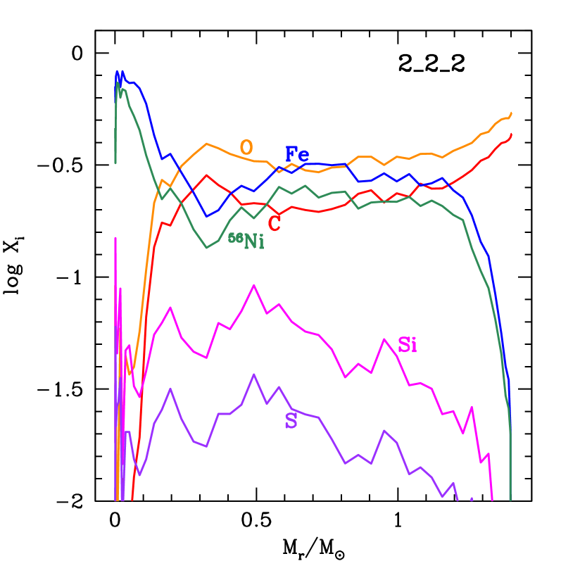
Figure 1: Mass fractions of the most abundant elements produced in model 2_2_2 as a function of Lagrangian mass. Note ‘Fe’ includes iron-peak elements together with ⁵⁶Ni.

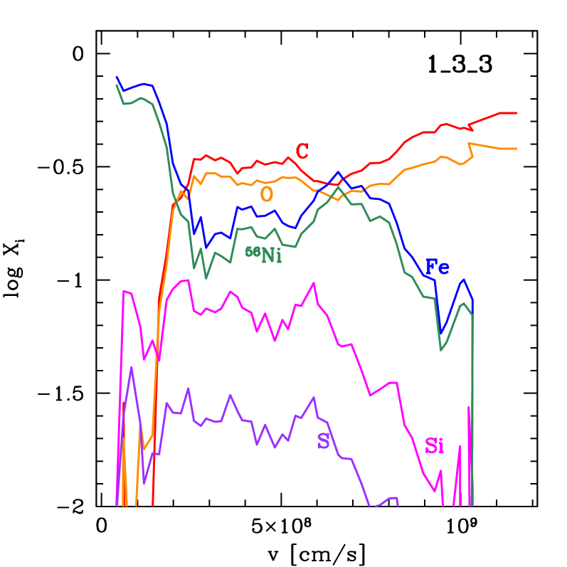
Figure 2: Mass fractions of most abundant elements for the model 1_3_3 as a function of the material velocity.

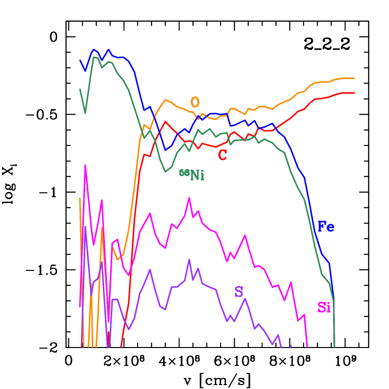
Figure 3: Mass fractions of the most abundant elements produced in model 2_2_2 as a function of material velocity. Note ‘Fe’ includes iron-peak elements together with ⁵⁶Ni.

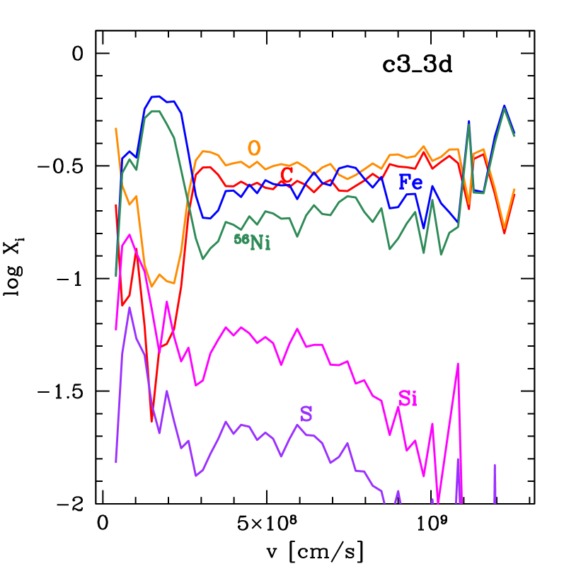
Figure 4: Mass fractions of most abundant elements for the model c3_3d as a function of the material velocity. Note ‘Fe’ includes iron-peak elements together with ⁵⁶Ni.

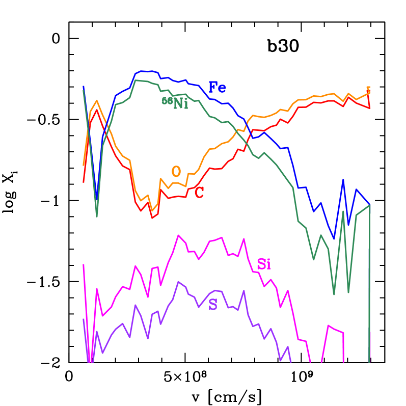
Figure 5: Mass fractions of most abundant elements for the model b30 as a function of the material velocity.

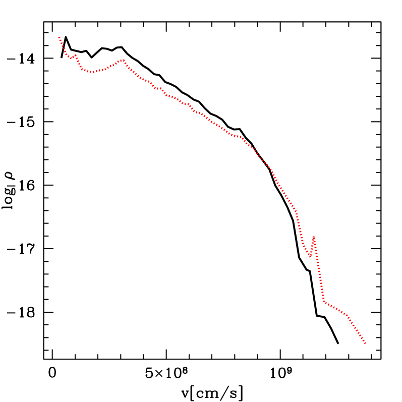
Figure 6: Initial ($t=10^{4}$ sec, black solid) and final ($t=90$ days, dotted) density profiles as a function of material velocity scaled to the same maximum for c3_3d.

4 Predicted observables and their diversity

Observations of SNe Ia indicate that a valid explosion model should release $\sim$$10^{51}$ erg of energy and synthesize $\sim 0.4\ldots 0.7\,M_{\sun}$ of ⁵⁶Ni. However, there exists a large diversity in the observations ranging from the class of sub-luminous SNe Ia (SN 1991bg) to the bright events (SN 1991T). The deflagration models use in this study release $4.4\ldots 6.3\times 10^{50}\,\mathrm{erg}$ of asymptotic kinetic energy into the ejecta and produce $0.24\ldots 0.42\,M_{\sun}$ of ⁵⁶Ni (see Table 2). Thus they fall into the lower range of observational expectations, but as of yet, do not account for the more luminous events.

The synthetic light curves are sensitive to the energy release, the ⁵⁶Ni production and the distribution of elements in the ejecta. Fig. 7 displays the computed $B$- and $V$-band light curves for all four of the explosion models (see Table 1). During maximum light these two passbands carry the main contribution to the luminosity. It is clear that in spite of modest values of explosion energy and ⁵⁶Ni mass, these deflagration models quite nicely reproduce the observed absolute peak $B$- and $V$-band magnitudes and decline rates of observed weak and normal SN Ia. Below we compare the computed light curves with some well-observed nearby SNe Ia.

4.1 Broad-band photometry

Detailed comparisons with observations of SN 1992A (Suntzeff, 1996) and SN 1994D (Richmond et al., 1995; Meikle et al., 1996; Smith et al., 2000) are presented in Figs. 8-11. These two SN Ia were selected because they are both well observed and the ⁵⁶Ni masses derived for each of them (Stritzinger, 2005) are similar to the values of the models. The observational template light curves are obtained as described in Contardo et al. (2000) and Stritzinger & Leibundgut (2005). The filter transmission functions used to derive the light curves from the modeled spectrum are from Stritzinger et al. (2005). The zero time on the plots is for the time of $B$-band maximum (both for theory and observations).

In Fig. 8 we compare synthetic light curves derived from model 1_3_3 (Röpke et al. 2005) with observations of SN 1994D. The distance to SN 1994D is still controversial. We have assumed the distance modulus 30.4 from (Drenkhahn & Richtler 1999) and the total reddening assumed is E(B-V)_tot$=$$0.022$

The model produced only $0.24\,M_{\odot}$ of ⁵⁶Ni, that is why the modeled $UBV$-band maxima are low compared with SN 1994D. The decline in $B$-band light curve for 15 days after the maximum light is also slow for a low luminosity SN Ia. The near infrared maxima are of the correct order, although they lack a convincing secondary maxima.

In Fig. 9 we compare computed light curves derived from model 2_2_2 (Röpke et al. 2005) with observations of SN 1992A. The distance modulus is taken to be 31.35 and the observed light curves are de-reddened assuming E(B-V)_tot$=$$0.017$. Richtler et al. (2000) have shown that a number of different distance determinations of the Fornax cluster of galaxies (where SN 1992A is located) agree well with a distance modulus of 31.35$\pm$0.04 mag (18.6$\pm$0.3Mpc). Madore et al. (1998) have published a Cepheid distance to the cluster giving a distance modulus of 31.35 $\pm$ 0.07.

The model produced $0.3\,M_{\odot}$ of ⁵⁶Ni. This is not a sufficient amount to account for the peak $B$- and $V$-band magnitudes. However, the peak value in the $U$-band is almost reached, although somewhat earlier than what is required by the observations. The decline in the $B$- and $V$-bands and the shapes of $I$- and $R$-band light curves are similar to those for model 1_3_3.

Fig. 10 displays the theoretical light curves for model c3_3d as compared with observations of SN 1994D. The ⁵⁶Ni mass is rather low ($0.28\,M_{\odot}$) and the general behavior of the fluxes is similar to the previous cases.

The best agreement with observations in the $B$- and $V$-bands is achieved with model b30. Fig. 11 shows the synthetic light curves derived from model b30 with observations of SN 1992A. Near maximum light there is a very good (almost perfect) agreement in the $B$- and $V$-bands as well as in the decline rate 20 days past maximum. This is an important result for cosmological applications, since the decline rate in those passbands (which are the main contributors to luminosity at this epoch) is used for calibration of the absolute fluxes. The flux in the $U$-band peaks early while at the same time overshoots the observed peak luminosity, and then declines too fast. This behavior may be explained by the significant amount of mixing of $\rm{}^{56}Ni$ in model b30 (see Fig. 5). With a large fraction of mixed $\rm{}^{56}Ni$, one would expect an excess of $U$-band flux prior to maximum followed by a rapid evolution. Less mixing of $\rm{}^{56}Ni$ may help to put the model in a better agreement with observations. Note, however, the maximum $U$-band luminosity is on the correct order for SN 1994D.

Our experiments with other models show that a more layered structure of chemical composition may also help to produce secondary maxima in the $R-$ and $I$-bands, which are not reproduced by the strongly mixed model in Figs. 8-11. See Fig. 3. in Blinnikov & Sorokina (2004) for the abundance profile of the classical W7 model (Nomoto et al. 1984).

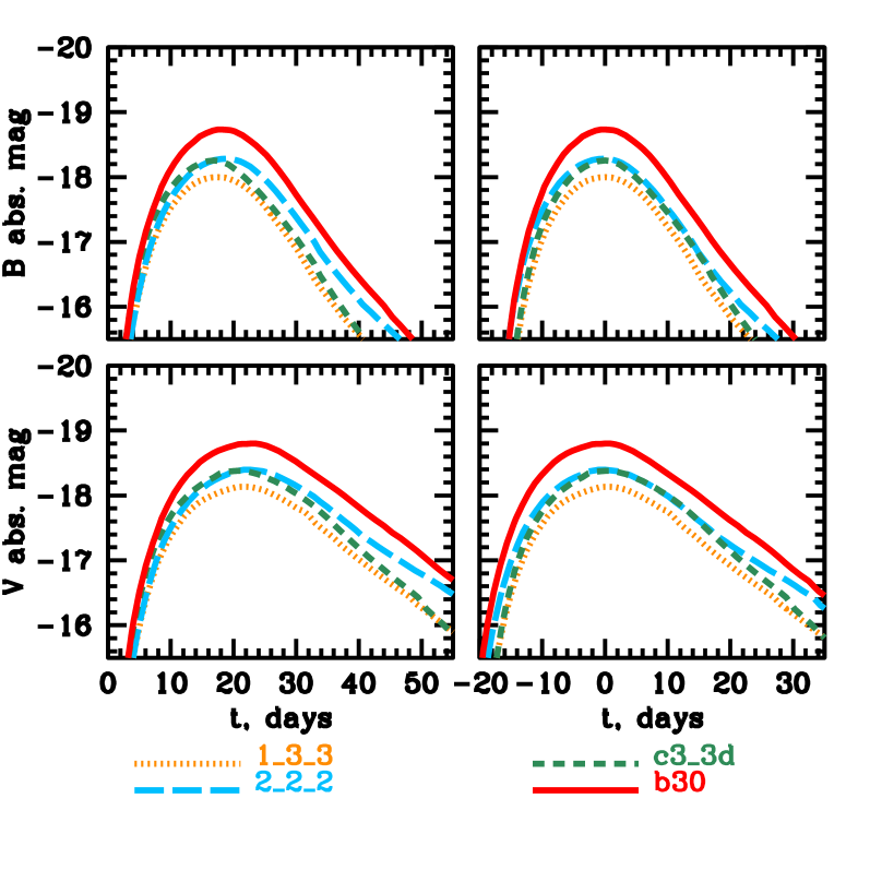
Figure 7: $B$- and $V$-band light curves for all 4 models. Left: zero time is the moment of explosion. Right: zero time is the maximum light in the given band.

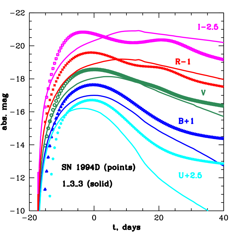
Figure 8: $UBVRI$ light curves for 1_3_3 compared with observations of SN1994D. Zero time is $B$-band maximum.

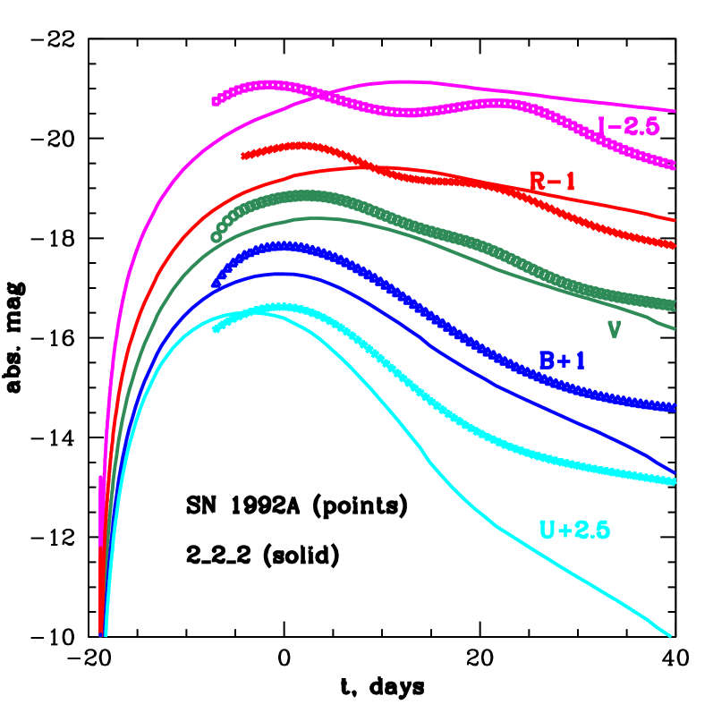
Figure 9: $UBVRI$ light curves for 2_2_2 compared with observed light curves from SN 1992A (data points). Zero time is $B$-band maximum.

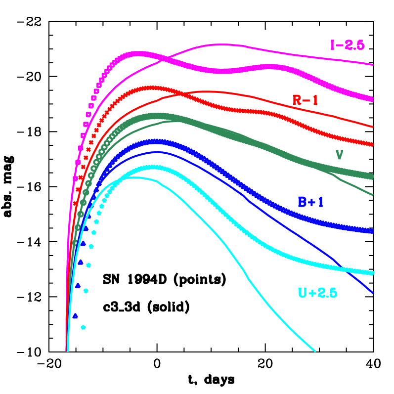
Figure 10: $UBVRI$ light curves for c3_3d and observations of SN1994D. Zero time is $B$-band maximum.

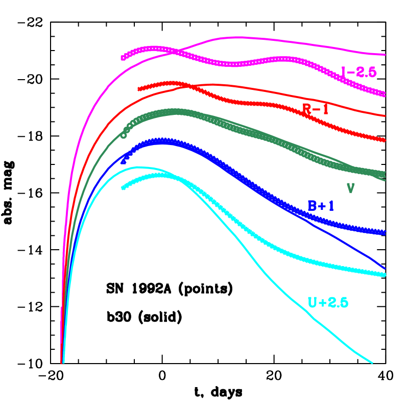
Figure 11: Synthetic light curves derived from model b30 (solid curves) (Travaglio et al. 2004) compared with observed light curves from SN 1992A (data points). Zero time is with respect to $B$-band maximum.

Some computed light curves parameters are summarized in Table 3. If we compare our results for $\Delta$m${}_{15}({\rm B})$ with the Phillips relation (Phillips et al. 1999), we find that model b30 fits quite well, while other lower ⁵⁶Ni mass models are somewhat under-luminous for their values of $\Delta$m${}_{15}({\rm B})$. In this comparison, one should take into account that we have used H${}_{\circ}=72$ km s^-1 Mpc^-1, while Phillips et al. (1999) used H${}_{\circ}=65$ km s^-1 Mpc^-1.

Table 3: Model $B$-band light curve rise-times and $\Delta$m${}_{15}({\rm B})$

model	$t_{\max}(B)$, days	$B_{\max}$	$\Delta$m${}_{15}(B)$
1_3_3	$17.58$	$-18.00$	$1.52$
2_2_2	$18.59$	$-18.28$	$1.40$
c3_3d	$16.96$	$-18.26$	$1.46$
b30	$18.18$	$-18.73$	$1.43$

4.2 Bolometric light curves

In Fig. 12 we compare the computed bolometric light curve for the model b30 with several of the UltraViolet Optical InfRared (UVOIR) light curves presented in Stritzinger (2005). Note that the theoretical bolometric light curve (dotted line) is computed in the wavelength range from extreme ultraviolet to far infrared. The templates UVOIR light curves are computed in the range from $U$-band (3100 Å) to the near infrared (10,000 Å). Therefore if we take a simple cut from the multi-group spectrum and sum the flux we obtain a UVOIR light curve (solid line in Fig. 12) that can be directly compared to the template UVOIR light curves. Although the luminosity at maximum and the rise-time are in good agreement with SN 1992A the decline rate is somewhat slower than observed. This is mostly due to the slow decline of the near infrared flux in the theoretical radiative model.

In Fig. 13 we compare the bolometric light derived from model c3_3d to the template UVOIR light curves. Compared to the previous model, c3_3d has a lower explosion energy and produces a smaller amount of ⁵⁶Ni (see Table 2). As a results we see that the total luminosity is less than what is determined from model b30.

In the next section we compare the UVOIR luminosity for our four models to the luminosities derived from the template light curves by the method presented in Stritzinger & Leibundgut (2005).

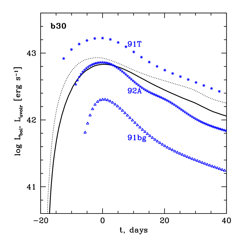
Figure 12: Total bolometric luminosity (dotted) and UVOIR luminosity (solid) for the model b30. Observations, shown for three representative SNe Ia, should be compared only with the solid line. Zero time is the epoch of maximum luminosity for each light curve.

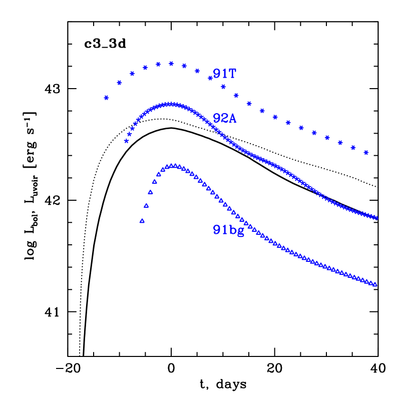
Figure 13: Bolometric luminosity (dotted) and UVOIR luminosity (solid) for the model c3_3d.

Figure 14: Deposited gamma-ray (solid line) and bolometric luminosity (dashes) for the model b30. Zero time is the explosion epoch.

4.3 Photospheric velocity

Our radiation hydro models allow us to evaluate the velocity of material at the level of the photosphere. We define this level as a layer with an optical depth of $2/3$ in the $BV$-bands. The results for the velocity at this level are shown in Fig. 15. We find that the photospheric velocity is near $\sim 10^{4}$ km s^-1 and changes weakly in the models, while observations sometimes show larger velocities before maximum followed by a faster evolution. For example, several days before $B$-band maximum the Si II $\lambda 6355$ absorption feature in SN 1992A indicated velocities on the order of $13\times 10^{3}$ km s^-1 (Kirshner et al. 1993). Moreover Patat et al. (1996) obtain for SN 1994D $14\times 10^{3}$ km s^-1 10 days before $B$-band maximum. Similar values are found by Branch et al. (2005), see Fig. 15. In both SNe Ia the velocity fell quickly near maximum light and stayed $\sim$10⁴ km s^-1 around day 20 after the maximum. Note, that in Fig. 15 the time is given from the explosion epoch, and epochs of $B$-band maximum are presented in Table 3.

Figure 15: Photospheric velocity for c3_3d (solid), 2_2_2 (dashed) and b30 (dotted) defined as $R_{\tau(BV)=2/3}/t$. Circles show the velocity at ‘Rosseland’ photosphere for b30. Crosses are the data for SN 1994D from Branch et al. 2005. Zero time is the explosion epoch.

It should be noted that Blondin et al. (2005) recently presented a detailed analysis of line profiles for a large sample of SNe Ia. Their study indicates that there are many nuances at play that make the procedure of using line profiles as a measure of photospheric velocities a difficult task. In addition some SNe Ia exhibit a very slow evolution of velocity measured by Si II $\lambda 6355$ absorption near $\sim 10^{4}$ km s^-1, see Fig. 6 in (Blondin et al., 2005).

This may be interpreted as the signature of lower bound of Si distribution (e.g., Branch et al., 2005), not as the signature of the slow evolution of the photospheric velocity. To illustrate this we plot in Fig. 15 the behaviour of the velocity on the photosphere determined by the Rosseland mean opacity for b30. While the the ejecta cool down after the maximum light the Rosseland opacity is determined by red wavelengths where the matter is more transparent than in blue. Here the photospheric velocity goes down monotonically which is usually observed in spectroscopic studies. The non-monotonic behaviour of the photospheric velocity in Fig. 15 may be explained by different level of excitation caused by the presence of Ni56 in outer layers. This may be enough to support optical depth in bluer wavelengths, but not sufficient for a ‘true’ photosphere.

The observation of fast features in the spectra of some SNe Ia demonstrates the need for further development of the deflagration models. Our procedure of averaging of the original 3-D models over solid angles somewhat suppresses the fastest motions. As a result the outermost mesh zone in model b30 contains a mass of $8.5\times 10^{-4}M_{\sun}$ with an asymptotic velocity $12.98\times 10^{3}$ km s^-1, while some of the tracer particles of the 3-D model had $13.81\times 10^{3}$ km s^-1.

5 Deriving ⁵⁶Ni masses from SNe Ia light curves

Following “Arnett’s rule” (Arnett 1979, 1982) one can derive the ⁵⁶Ni mass from the peak luminosity of a SN Ia. Arnett’s rule simply states that at the epoch of maximum light the peak luminosity is equal to the rate of gamma-ray deposition inside the ejecta. The derivation of this statement is based on many simplifying assumptions, yet it is well satisfied in the current set of models (see Fig. 14).

To derive a ⁵⁶Ni mass from the peak luminosity one also has to know the fraction of the total radioactive power that is actually deposited, and the fraction that escapes. An empirical procedure for finding the ⁵⁶Ni mass has been developed by Stritzinger & Leibundgut (2005). With a UVOIR light curve and the simple relation $L_{\rm max}=2\times 10^{43}M_{\rm Ni}/M{\sun}$ erg s^-1, (and 10% correction taking into account the difference of UVOIR and bolometric luminosity) they were able to make estimates of the $\rm{}^{56}Ni$ mass for a large number of SNe Ia.

The accuracy of this procedure may be tested with our synthetic light curves. Fig. 16 contains the comparison of the UVOIR light curve derived from theoretical $UBVRI$ fluxes applying the procedure of Stritzinger & Leibundgut with the results for model b30.

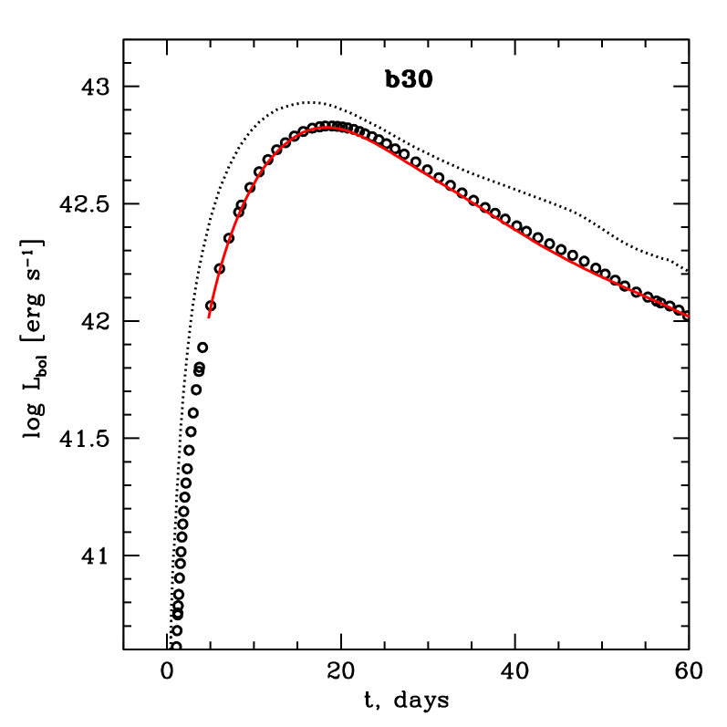
Figure 16: Computed UVOIR light curve for the model b30 (circles) compared with the UVOIR light curve derived using the procedure of Stritzinger & Leibundgut (2005) (solid line) with the modeled $UBVRI$ light curves. The full bolometric luminosity is given by the dotted line. Zero time is the explosion epoch.

Table 4 shows that the derived mass of ⁵⁶Ni is systematically lower than the actual values in the models. Fig. 17 explains the reason for this: the relation $L_{\rm max}=2\times 10^{43}M_{\rm Ni}/M{\sun}$ erg s^-1 is good for true (total) bolometric luminosity which is systematically higher than the UVOIR luminosity and the 10% correction is a bit small to fully account for that.

The model b30 produced $0.42$ M_☉ of ⁵⁶Ni and a comparable value of $0.40$ M_☉ of ⁵⁶Ni was found for SN 1992A by Stritzinger (2005). The agreement is better, than suggested by numbers in the Table 4, because the observed UVOIR luminosity at maximum light is somewhat higher than in the model b30, since our models have IR fluxes too low at UVOIR maximum light (see Figs. 11and 12).

Figure 17: Peak values of UVOIR (stars) and bolometric (circles) luminosity versus ⁵⁶Ni mass in logarithmic scale for our four models. Solid line is the relation from (Stritzinger & Leibundgut, 2005). Dashed arrow points to the correct value of ⁵⁶Ni mass for b30. Thin solid line with arrow points to the lower ⁵⁶Ni mass found from UVOIR luminosity and thick solid arrow is 10% correction used (according to Stritzinger & Leibundgut, 2005) to obtain the number given in the Table 4.

Table 4: Values of ⁵⁶Ni mass derived from the theoretical light curves by the method from Stritzinger & Leibundgut (2005) .

model	$\log L_{\max}$, erg s-1	$M(^{56}\textrm{Ni})[M_{\sun}]$,	$M(^{56}\textrm{Ni})[M_{\sun}]$,
		actual	derived
1_3_3	$42.579$	$0.24$	$0.21$
2_2_2	$42.681$	$0.31$	$0.26$
c3_3d	$42.636$	$0.28$	$0.23$
b30	$42.821$	$0.42$	$0.37$

6 Discussion of the results

This study does not produce theoretical light curves that perfectly match all the observations. However, the synthetic modeled $UBV$ light curves do show good agreement with the observed ones for modestly luminous SNe Ia, although the evolution of the luminosity is somewhat slower (particularly in the bolometric light curve) than observed. In this section we discuss the approximations made in the current study and their probable influence on the results.

6.1 Shortcomings of the current modeling

Partially, the remaining differences between synthetic and observed light curves can be attributed to the the explosion models. All centrally ignited models possess an artificial flame ignition configuration that is known to give rise to weak explosions. In addition in the four explosion models used, thermonuclear burning was not followed below densities of 10⁷ g cm^-3. In a more realistic explosion model burning should continue to far lower densities. This has two effects that are likely to improve the agreement between the modeled and observed light curves. First, at lower densities more intermediate mass elements (IMEs) (e.g. Si, S, and Ca) will be produced which are clearly under-abundant in the current set of models. Second, burning to lower densities releases more nuclear energy resulting in higher expansion velocities. Currently work is in progress to analyze the effects of extending the burning to lower fuel densities (see Röpke & Hillebrandt, 2005a).

It is clear that the radiative transfer models need considerable improvement at certain points. While up to 20 days after the maximum light we find good agreement of the best model with observations in the $B$- and $V$- bands, it is clear that at later epochs large deviations are present. During these epochs when the SN Ia ejecta enter the nebular phase, the LTE assumption is clearly not valid. In addition, the procedure of averaging a 3-D model for 1-D transport can introduce an error which can only be corrected in a full 3-D radiative transfer simulations.

Another factor that has a dramatic influence on the modeled light curves is the treatment of the opacity. Direct numerical summation of individual lines, as done in atmospheric codes like phoenix (Baron et al. 1996b) may be dangerous in deep interiors of SN ejecta, since the difference of the source function and mean intensity is very small where the lines are strong. The subtraction of the nearly equal numbers always leads to loss of accuracy, and the result significantly depends on the order of summation of lines: one has to start from the weakest ones (cf. Sorokina & Blinnikov 2002). Opacity sampling (OS) or opacity distribution function (ODF) and $k$-distribution procedures used in static atmospheres must be modified for applications in supernova envelopes (Wehrse et al. 2002). However, the recipes for the statistical treatment of lines were developed by Wehrse et al. (2002) only for the flux equation, and at present it is unclear how to generalize them for treatment with the energy equation, e.g. Eq. (3). A deterministic approach for an average expansion opacity to be used in the energy equation was previously developed (Sorokina & Blinnikov 2002), but it is more computationally demanding compared to the simple formulae (Eastman & Pinto 1993) employed in this study.

For some runs in the current set of models we have applied the new recipes by Sorokina & Blinnikov (2002) and found for them a small difference in comparison with the prescription by Eastman & Pinto (1993). This is probably due to strong mixing of the models. More layered models produce clear secondary maxima in the $R$- and $I$- bands, and the use of ‘new’ opacities from Sorokina & Blinnikov (2002) makes them more pronounced.

Recent papers by Branch et al. (2005); Stehle et al. (2005) used spectroscopic analysis in different approximations and found that the composition structure in SNe Ia is stratified but has some degree of mixing. The latter is not so strong as the mixing in the current models. This is another hint for need of producing more chemical stratification in the hydrodynamic models. However, one should first build detailed NLTE spectroscopic models for the current models. The line spectra are sensitive not only to the distribution of chemical elements but also to the conditions of excitation which may change in radius in more pronounced way than the chemical composition.

The absolute magnitudes for SNe Ia in the infrared $J,H$ and $K$-bands is very uniform even for peculiar events (Krisciunas et al. 2001, 2004). This is a rather puzzling result given the variety of morphologies displayed in the $R$- and $I$- bands. The opacity physics in our radiation hydro model is presently not complete in the $J,H$ and $K$-bands and it will be necessary to address this problem in future work.

6.2 Hydrodynamic effects in SN Ia

Progenitors of SNe Ia are believed to be compact degenerate stars. The explosion develops on a time-scale of a second, and homologous expansion should be a good approximation after a few seconds. This approximation is usually exploited in the radiative transfer codes that neglect hydrodynamics (Eastman & Pinto 1993; Lucy 2005). However, Pinto & Eastman (2000a) pointed out that the energy released in the ⁵⁶Ni decay can influence the dynamics of the expansion. The ⁵⁶Ni decay energy is $3\times 10^{16}$erg g^-1 which is equivalent to a speed of $2.5\times 10^{3}$ km s^-1, if transformed to the kinetic energy of a gram of material. Pinto & Eastman (2000a) state “Since the observed expansion velocity of SNe Ia is in excess of $10^{4}$ km s^-1, we expect that this additional source of energy will have a modest, but perhaps not completely negligible, effect upon the velocity structure.”

In reality the heat released by the ⁵⁶Ni decay will not all go into the expansion of the SN Ia. If the majority of ⁵⁶Ni is located in the central regions of the ejecta then the main effect is an increase in the entropy and local pressure (both quantities are dominated by photons in the ejecta for the first several week). The weak overpressure will lead to a small decrease in density at the location of the ‘nickel bubble’, as well as to some acceleration of matter outside the bubble. It is often said that the expansion of the ejecta is supersonic and pressure cannot change the velocity of the matter, but one should remember that in the vicinity of each material point we have a ‘Hubble’ flow so differential velocities are in fact subsonic in a finite volume around each point.

In the case of a more uniform distribution of ⁵⁶Ni, like in the models under consideration, we should not expect the formation of a nickel bubble, but the general effect upon the velocity should be anticipated.

In order to compute the hydrodynamics correctly to find small deviations from homologous expansion we should not assume that energy conservation can be simplified to the condition of thermal equilibrium, and that the gas terms $dU+pdV$ can be neglected. This simplification, when the term $4\pi\int_{0}^{\infty}(\eta_{\nu}-\alpha_{\nu}J_{\nu})d\nu$ in the co-moving frame is equal to the rate of radioactive energy deposition $\varepsilon$ is always done in models that assume homologous expansion (Arnett 1980; Pinto & Eastman 2000a; Lucy 2005).

We do not make simplifying approximations such as neglecting the gas terms $dU+pdV$, nor do we assume homologous expansion. Eq. (3) automatically accounts for any deviations from thermal equilibrium.

The effect is modest, but as expected it may result in a $\sim$$10$% difference in velocity. This effect is evident for the c3_3d model (see Fig. 6). The solid black line is the initial model scaled to our result at 90 days since explosion. We see that the density profile has changed due to the ⁵⁶Ni and ⁵⁶Co decays; it clearly deviates from homology. The growth of the velocity in outer layers is also visible. The effect upon the total kinetic energy is smaller (see Table 2).

All of the models considered here have strongly mixed ⁵⁶Ni. Other models, with modest mixing do not show appreciable increase of the velocity in outer layers, but they demonstrate that the nickel bubble, i.e. the depression of density in ⁵⁶Ni-rich layers, continues to grow during the coasting stage. The change of the density is important for the deposition of gamma-ray energy, and this is reflected in the light curve.

6.3 Secondary maxima in $R$, $I$.

Most SNe Ia (except for subluminous SN 1991bg-like ones) display pronounced secondary maxima in their near-infrared and infrared light curves. Observations show a large variety of observed infrared maxima. According to Nobili et al. (2005), the light curve in $I$-band can peak before, as well as after $B_{\rm max}$ (between $-3$ days and $+3$ days with respect to $B_{\rm max}$). On average, the secondary maxima occurs 23.6 after the $B_{\rm max}$ with a dispersion of $\sigma=4.4$ days. However, there are strong arguments that this behavior is not random. Nobili et al. (2005) found a correlation between the time of the secondary peak and the $B$-band stretch parameter. A luminosity-width relation was also found between the peak $I$-band magnitude and the $B$- and $I$-band stretch parameter. Contardo et al. (2000) found some similar correlations between the strength of the secondary maximum and times of derivatives of the light curve.

This is a very interesting and long-standing problem for the theory of light curves. Although Eastman (1997) previously demonstrated that some models do produce a secondary infrared maxima (in that case it was a sub-Chandrasekhar model), the theory is still far from providing robust predictions concerning the shape of $I$-band light curve and the correlations pointed out in Nobili et al. (2005).

For example, Höflich (1995) found a weak secondary maxima for W7, and rather noisy $I$-band light curves for other models. Pinto & Eastman (2000b) also found rather weak secondary maxima, depending strongly on the atomic line database, nevertheless Eastman (1997) and Pinto & Eastman (2000b) have presented a physical argument that attempts to explain the observed secondary maxima. According to them, after $\sim$ 20 days past maximum light, when the monochromatic opacity in the near infrared becomes small due to recombination of higher ions, there exists a large amounts of singly ionized emitters (e.g. Ca II, Fe II, and Co II). Through fluorescence these lines cause an enhanced ‘leakage’ of previously trapped photons, thus giving rise to the secondary maxima.

For this mechanism to produce a secondary maxima the SN Ia model must require a large mass fraction of Ca, Fe, and Co located in central layers that are emitting photons near 20 days past maximum light. Too strong mixing of iron-peak elements reduces their amount in the center. With the MPA models the total mass of Ca is relatively small. Model b30 has 0.0037 M_☉ of Ca, while DD4 contains 0.0375 M_☉ (Pinto & Eastman 2000b) and W7 contains 0.025 M_☉; the latter two containing an order of magnitude more!

As previously mentioned, less pronounced mixing may allow model b30 to produce $R$- and $I$-band light curves that agree with the observation more closely. With less mixing of Fe-group elements and IMEs like Ca, our models may produce $R$- and $I$- band secondary maxima. This may also lead to a delay in the $U$-band rise-time.

What should be changed in the deflagration models to decrease the degree of the mixing, but at the same time to increase the amount of ⁵⁶Ni? We believe that the only feasible way is to lower the ignition density considerably. This will have two effects. First, electron captures become unimportant, increasing the ⁵⁶Ni at the expense of the other NSE nuclei. Secondly, at low densities the ¹²C-¹²C burning rate is low, too, and the heat diffusion time gets longer, thus reducing the laminar burning speed and giving the star more time to expand before rapid turbulent burning sets in. This should in fact also reduce the amount of mixing. These conjectures have to be tested in future detailed numerical modeling.

7 Conclusions

How the diversity of local SNe Ia can affect their use as distance indicators and the possibility of systematic trends (as a function of redshift) in their observed properties cannot be addressed without detailed radiative transfer modeling.

The set of hydrodynamical models used in this studied synthesized modest amounts of ⁵⁶Ni $\sim$0.3 - 0.4 M_☉ and displayed relatively low explosion energies (lower than the ‘standard’ 1.5 foe expected for a ‘typical’ SN Ia). However, our results show that Chandrasekhar mass models that burn by a pure deflagration do produce both $UBV$ light curves and photospheric expansion velocities that match well with observed weak to normal SNe Ia. As the majority of flux during maximum light is emitted within these passbands this is an encouraging result. Moreover, it is these passbands that are of great importance for cosmological applications of SNe Ia. It is clear that the models require some improvement in explaining the shapes of the near infrared light curves and in explaining fast spectral features that are observed in many normal events. The bolometric light curves calculated from our deflagration models evolve slightly slower than what is indicated from observations. These discrepancies hint at the necessity of producing faster moving ejecta, and somewhat less mixed chemical composition. The latest deflagration (to be discussed in a subsequent publication) models are promising in this aspect.

From the point of view of radiative transfer modeling several issues must be dealt with including: (1) determining the sensitivity of the results to the completeness of the atomic line data base, (2) the robustness of the various approximations employed such as the expansion opacity prescriptions, and (3) determining the importance of (time-dependent!) NLTE effects. These issues are currently being addressed and small steps are being made to bring us closer to a full 3-D transport model for SNe Ia.