Radio and infrared recombination studies of the southern massive star-forming region G333.6$-$0.2

Abstract

We present high spatial resolution radio and near-infrared hydrogen recombination line observations of the southern massive star-forming region G333.6$-$0.2. The 3.4-cm continuum peak is found slightly offset from the infrared source. The H90$\alpha$ spectra show for the first time a double peak profile at some positions. The complex velocity structure may be accounted for by champagne outflows, which may also explain the offset between the radio and infrared sources. The 2.17-$\mu$m Br$\gamma$ image and H90$\alpha$ map are combined to construct an extinction map which shows a trend probably set by the blister nature of the H ii region. The total number of Lyman continuum photons in the central 50-arcsec is estimated to be equivalent to that emitted by up to 19 O7V stars.

1 Introduction

G333.6$-$0.2 is a southern compact H ii region which was initially detected as one of the brightest radio sources in a 5-GHz Galactic plane survey (Goss & Shaver 1970). Radio recombination lines (RRLs) H90$\alpha$ and He90$\alpha$ were observed by McGee, Newton & Batchelor (1975), and McGee & Newton (1981) examined H76$\alpha$ and He76$\alpha$ RRLs. Both papers reported a Local Thermal Equilibrium (LTE) electron temperature ($T_{e}^{*}$) of slightly less than 7000 K and a ratio of singly ionised helium to singly ionised hydrogen [$Y^{+}=\frac{N({\rm He}^{+})}{N({\rm H}^{+})}$] of less than the solar value (i.e., $<10$ per cent). The H ii region is almost totally obscured in the visible ($A_{V}=18.5$, Landini et al. 1984) but is bright at infrared (IR) wavelengths, and has been studied intensively in this region of the spectrum (e.g. Aitken, Griffiths & Jones 1977; Hyland et al. 1980; Fujiyoshi et al. 1998, 2001, 2005, hereafter Papers 1, 2, and 3, respectively). In Paper 1, it was found that the H ii region must be excited by a cluster of O and B stars, rather than by a single star. Indeed, near-IR (NIR) broadband imaging revealed multiple point sources in G333.6$-$0.2 (Paper 3). Point sources with significant $H-K$ colour excess were found preferentially in extended emission regions and it was suggested that these red objects were physically associated with the H ii region. The powerful nature of this nebula was unveiled by mid-IR (MIR) imaging polarimetry (Paper 2) which showed bent magnetic field lines possibly shaped by the expansion of the ionised gas.

At radio wavelengths the most intense emission from H ii regions is caused by interactions between unbound charged particles, better known as free-free radiation or bremsstrahlung (braking radiation). Since the particles are free and their energy states are not quantised the radiation resulting from changes in their kinetic energy is continuous. Free-free emission is dominated by interactions of free electrons with the most abundant element, singly ionised hydrogen. Observations of the radio free-free emission (where extinction is usually negligible) can be used to predict the hydrogen recombination line fluxes at IR wavelengths, which in turn can be compared to the observed values to estimate extinction at the line wavelengths.

In this paper, we present radio synthesis observations at 3.4 cm, and the 2.17-$\mu$m Br$\gamma$ hydrogen recombination line imaging of G333.6$-$0.2. High spatial resolution data provided by radio interferometry can be compared directly with those at NIR wavelengths to infer spatial variation of extinction across the face of the H ii region. The H90$\alpha$ RRL, observed both at high spatial and spectral resolution, is used as a probe of the physical conditions in the emitting gas.

2 Observations and data reduction

2.1 Radio observations

The radio observations were made on 1996 October 8 at the Australia Telescope Compact Array (ATCA) in Narrabri, Australia. The ATCA is a synthesis telescope which consists of six 22-m antennae on a 6-km east-west track. One set of measurements was taken with the baseline configuration 6A. The longest baseline of 6 km was chosen to give the final map the highest possible spatial resolution available with the ATCA.

G333.6$-$0.2 was observed at a frequency centred between the H90$\alpha$ (rest frequency 8.872 GHz) and He90$\alpha$ (8.876 GHz) RRLs. Each of two orthogonal polarisations was recorded, using a correlator configuration of 512 channels covering a 16-MHz bandwidth. The primary calibrator (1934$-$638; 2.8 Jy at 8.8 GHz with an uncertainty of up to a few per cent) was observed for 20 minutes during the run for the bandpass correction and the flux calibration. A secondary calibrator (1619$-$680) was observed every 20 minutes for 5 minutes throughout the observation period for position and phase calibration.

Data reduction was carried out using the software package MIRIAD. The continuum and H90$\alpha$ RRL maps were constructed using natural weighting in the conventional Fast Fourier Transformation. The maps were then deconvolved using the CLEAN routine in MIRIAD. Spectral cubes were also made following the same method; however, in order to improve the signal-to-noise ratio ($S/N$), 4 consecutive channels were binned together resulting in an effective velocity resolution of $\sim 4$ km s^-1. The cleaned maps were finally restored to intensity maps with a 1.6-arcsec diameter circular beam, which therefore is the effective spatial resolution of the maps presented here.

2.1.1 Missing flux from extended structures

McGee et al. (1975) observed G333.6$-$0.2 as part of their H90$\alpha$ RRL survey of bright southern radio sources. Using a 2.5-arcmin beam they measured the 3.4-cm continuum flux density of $80\pm 17$ Jy. However, in our continuum map the integrated total flux density in an area $\sim 2\times 2$ arcmin² was found to be only $\sim 13$ Jy.

Lack of short baselines in interferometry leads to the loss of sensitivity to extended structures. The ATCA 6A configuration has a shortest baseline of 337 m, and thus at 3.4 cm is not responsive to structure smoothly distributed on a scale of $\sim 30$ arcsec or larger. The target is a compact H ii region whose IR counterpart has a core-halo geometry (Aitken et al. 1977) in which most flux is concentrated in the central region. We have assumed that the missing extended emission underlying the compact H ii region takes the shape of a 2-D Gaussian. Its peak value and full widths at half maximum (FWHMs) are adjusted so that it would contain the missing flux and satisfy the level of extinction measured by Landini et al. (1984) (see Section 3.2.1 for details).

2.2 NIR observations

The NIR observations of G333.6$-$0.2 were carried out on 1995 August 11. All measurements were obtained using the IR imaging spectrometer IRIS at the $f/36$ Cassegrain focus of the 3.9-m Anglo-Australian Telescope (AAT), Siding Spring, Australia. The detector element of IRIS is a Rockwell $128\times 128$ HgCdTe NICMOS2 array, which is housed in a closed-cycle compressed helium refrigeration unit. In the imaging mode, wavelength selection is provided by discrete filters such as ‘standard’ NIR broadband ($J,H,K$). A more complete description of the instrument can be found in Allen et al. (1993).

Table 1 summarises the NIR observations of G333.6$-$0.2. INTERM mode was used to give a pixel size of $\sim 0.25\times 0.25$ arcsec². The object was dithered in the instrument’s field of view, which produced the final image size of $\sim 50\times 50$ arcsec². The 2.25-$\mu$m H₂(2$-$1) S(1) image was used for subtracting the continuum from the 2.17-$\mu$m Br$\gamma$ image. Moneti & Moorwood (1989) found that G333.6$-$0.2 showed only a weak H₂(1$-$0) S(1) emission in the central region [$I_{{\rm Br}\gamma}=3.5\times 10^{-18}$ W cm^-2 and $I_{(1-0)}=1.3\times 10^{-20}$ W cm^-2, both measured in a $6\times 6$-arcsec² beam]. In conditions characteristic of H ii regions, the (1$-$0) mode is always much stronger than the (2$-$1) (e.g. Burton 1992). We therefore assumed that the (2$-$1) image contained only the continuum emission. The calibration was achieved by observing the standard star SA94$-$251 ($K=8.305$, Carter & Meadows 1995). Seeing on the night was quite good and observations of standard stars showed FWHMs of about 0.6 arcsec.

Table 1: Summary of NIR observations of G333.6$-$0.2.

Date	Filter	$\lambda_{0}$	$\Delta\lambda$	Integration
		($\mu$m)		(sec/position)
11 Aug 1995	Br$\gamma$	2.17	1 %	$2\times 10.0$
	H2(2$-$1) S(1)	2.25	1 %	$1\times 10.0$

3 Results and discussions

3.1 Radio data

3.1.1 The 3.4-cm continuum

Figure 1 shows the 3.4-cm continuum map. The overall similarity to the IR images (cf. Figure 7. See also Papers 1 & 3) is quite remarkable. It is dominated by a north-south elongated main peak in the centre with steeper gradient to the east. Hyland et al. (1980) suggested that this steep gradient may be caused by extinction. Indeed, the extinction map (see Section 3.2.1) shows a slight increase of extinction in this direction. An arm-like extension, which was described as the secondary peak in Papers 1 & 3, is seen about 5 arcsec to the east of the main peak. The gap between the main and secondary peaks is also present. As the gap is still present at 3.4 cm, it is likely that the main and secondary peaks are separate ionised regions and the gap represents a narrow non-ionized region in between, rather than an apparent structure simply caused by a heavy foreground extinction. It was suggested in Paper 3 that both main and secondary peaks house exciting sources.

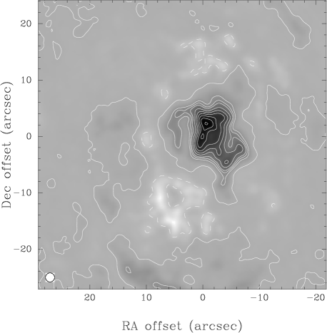
Figure 1: The 3.4-cm continuum grey-scale map of G333.6$-$0.2. Contours are drawn at $-$0.050 (broken line), 0.00050, 0.10, 0.15, 0.20, 0.30, 0.40, 0.50, 0.60, 0.70, and 0.79 Jy beam^-1. Axis offsets are from the MIR main peak position [${\rm RA}=16^{{\rm h}}22^{{\rm m}}09.\!\!^{{\rm s}}6$ and ${\rm Dec}=-50^{\circ}06^{\prime}00^{\prime\prime}$ (J2000)]. The circular 1.6-arcsec diameter synthesised beam is also shown at the bottom left hand corner.

The most significant difference between the IR and radio continuum images is that the radio continuum main peak is found offset slightly ($\sim 2$ arcsec) from the MIR main peak position. The coordinates of the radio main peak are ${\rm RA}=16^{{\rm h}}22^{{\rm m}}09.\!\!^{{\rm s}}5$ and ${\rm Dec}=-50^{\circ}05^{\prime}58^{\prime\prime}$ (J2000). The size of the source, determined by fitting a 2-D Gaussian profile, is 4.9 arcsec in RA and 6.9 arcsec in Dec, or about 0.086 pc $\sim 1.8\times 10^{4}$ au at 3.0 kpc (an assumed distance to G333.6$-$0.2, Colgan et al. 1993). There is a ridge running to the south (and slightly east) from the main continuum peak and in fact the MIR main peak position coincides with the peak on this ridge.

3.1.2 The H90$\alpha$ RRL

The H90$\alpha$ RRL map is presented in Figure 2. It shows the spatial variation of the integral over velocity of the recombination line. The distribution of the RRL emission is similar to that of the 3.4-cm continuum. The size of the H90$\alpha$ peak emission, which is coincident with the peak of the 3.4-cm continuum emission, measured again by fitting a 2-D Gaussian profile, is 4.1 arcsec in RA and 5.7 arcsec in Dec, which is only slightly smaller than the size of the continuum peak. There is also a ridge running to the south of the main peak; however, the peak on the ridge is slightly more south-east (by about 1 arcsec south and 0.5 arcsec east) than the ridge peak position in the 3.4-cm continuum map.

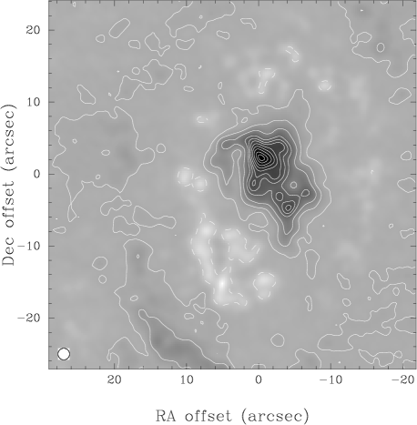
Figure 2: The H90$\alpha$ grey-scale map of G333.6$-$0.2. Contours are drawn at $-$0.25 (broken line), 0.025, 0.25, 0.65, 1.3, 1.7, 2.1, 2.5, 3.0, 3.5, 4.0, 4.3 Jy$\cdot$km s^-1 beam^-1. The coordinates of the origin are as in Figure 1.

Figure 3 shows the total H90$\alpha$ RRL spectrum in the central $\sim 2\times 2$ arcmin². Attempts were made to fit either a single or a double Gaussian profile to the spectrum and it was found that a combination of two Gaussian functions gave a better fit (the sum of fitting residuals was smaller). As it will be shown later, G333.6$-$0.2 exhibits a complex velocity structure with some positions displaying a double peak spectrum. Such a structure has never been observed with large-beam, single-dish radio studies of the H ii region and this emphasises the importance of high spatial resolution investigations.

The parameters derived from the fit are summarised in Table 2. All velocities refer to the Local Standard of Rest (LSR) frame. The weak broad feature centred at around $-270$ km s^-1 is the H113$\beta$ RRL. Additional weak emission may be present at about $-150$ km s^-1 and could be the He90$\alpha$ RRL, although it would normally be expected at a bluer velocity [$\sim-175$ km s^-1, cf. Figure 1(o), McGee et al. (1975)]. It should be noted, however, that both lines presumably also exhibit double peak spectra and therefore are likely to be blended. No attempt was made to fit parameters to these RRLs.

Figure 3: The total H90$\alpha$ spectrum in the central $\sim 2\times 2$ arcmin². It shows the data points (dots), a multiple (double) Gaussian fit to the data (solid line), and the residual (i.e., the difference between the actual data and the fit; dashed line).

Table 2: The Gaussian fit parameters to the total H90$\alpha$ spectrum in the central $\sim 2\times 2$ arcmin² (see Figure 3).

$S_{l}$	$V_{{\rm LSR}}$	$\Delta V_{G}$	Reference
(mJy)	(km s-1)	(km s-1)
$433\pm 117$	$-73.4\pm 3.1$	$26.3\pm 4.5$	This study
$798\pm 53$	$-45.6\pm 2.8$	$36.1\pm 4.2$	This study
	$-47.1\pm 0.2$	$43.9\pm 0.3$	McGee et al. (1975)

Table 2 also lists the single-dish H90$\alpha$ measurements of McGee et al. (1975). The overall velocity of the ionized gas in G333.6$-$0.2 was found by three independent single-dish observations at different frequencies to be $\sim-46$ km s^-1. Apart from McGee et al. (1975), who found its velocity to be $-47.1$ km s^-1, McGee & Newton (1981) determined $-45.3$ km s^-1 from the 14.7-GHz H76$\alpha$ RRL observation with a 2.3-arcmin beam, and Caswell & Haynes (1987) obtained $-46$ km s^-1 by measuring the 5-GHz H109$\alpha$ and H110$\alpha$ RRLs with a $\sim 4$-arcmin beam. The redder ($\sim-46$ km s^-1) of the two velocity components we found above is therefore likely to be associated with emission from extended structures, most of which escaped detection in the current study (see Section 2.1.1). The bluer component at $\sim-70$ km s^-1, detected for the first time with high spatial resolution observations presented here, must then be originating from compact structures.

Figure 4 shows average spectra in $1.75\times 1.75$-arcsec² boxes in the central region superimposed on the 3.4-cm continuum map. The boxes are positioned so that they would be centred on the main peak and the peak on the ridge. Positions 34, 35, and 36 are centred on each of the three radio peaks in the south-west extension (see Figures 1 & 2). Figure 5 shows the H90$\alpha$ RRL spectra fitted with Gaussian profiles. Again, we determined whether each spectrum contains a single or a double line by fitting either a single or a double Gaussian profile and selecting the one that resulted in a smaller sum of residuals. Parameters found by the fit are summarised in Table 3.

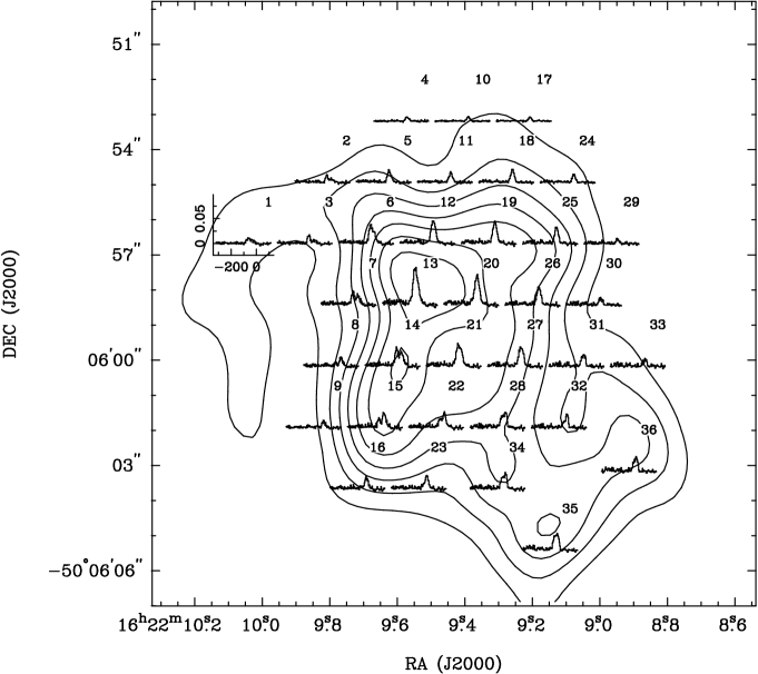
Figure 4: A grid of average spectra in $1.75\times 1.75$-arcsec² boxes superimposed on the 3.4-cm continuum map of G333.6$-$0.2. Contours are drawn from 0.1 Jy beam^-1 in an 0.1 Jy beam^-1 interval.

Figure 5: The H90$\alpha$ RRL spectra averaged in $1.75\times 1.75$-arcsec² boxes (see Figure 4). Each window shows data points (dots), a Gaussian profile fit to the data (solid line), and the number at the top left hand corner refers to the position number in Figure 4.

Table 3: The Gaussian fit parameters to the H90$\alpha$ RRL from the grid of $1.75\times 1.75$-arcsec² boxes (see Figure 5). The position numbers refer to those indicated in Figure 4. $S_{l}$ is in mJy beam^-1 and $n_{e}$ in $\times 10^{5}$ cm^-3.

No.	$S_{l}$	err	$V_{{\rm LSR}}$	err	$\Delta V_{G}$	err	$T_{e}^{*}$	$T_{b}$	$\tau_{c}$	$T_{e}$	err	$n_{e}$	$b_{n}$	$\beta_{n}$
			(km/s)		(km/s)		(K)	(K)		(K)
1	9.3	4.1	$-$65.7	7.4	35.8	9.8	4861	856	0.19	5000	4000	3.00	0.997977	$-$0.372641
	5.4	2.0	$-$29.4	18.8	46.1	30.1
2	14.0	1.2	$-$68.1	0.9	20.3	2.2	3166	488	0.17	3200	800	1.65	0.997272	$-$0.184034
	6.1	0.7	$-$31.4	3.7	42.3	9.1
3	16.9	1.2	$-$70.8	1.0	24.1	2.4	4477	883	0.22	4500	1200	4.58	0.998264	$-$0.069765
	6.3	1.0	$-$24.9	3.4	40.1	9.6
4	8.0	0.9	$-$59.4	2.5	21.1	4.2	3093	209	0.07	3100	1600	1.65	0.997268	$-$0.149526
	3.6	1.0	$-$38.7	5.0	19.5	9.3
5	23.7	1.3	$-$60.2	1.9	29.9	4.1	3834	935	0.27	3900	2100	2.51	0.997812	$-$0.160766
	6.6	2.7	$-$34.2	4.5	19.5	8.4
6	30.7	9.4	$-$69.7	2.7	27.7	4.2	4350	2269	0.59	5100	2100	1.90	0.997535	$-$0.691416
	21.8	3.8	$-$41.3	8.2	41.5	11.5
7	26.6	1.9	$-$68.7	1.3	27.1	3.0	4349	1773	0.47	4700	900	2.44	0.997793	$-$0.404504
	18.1	1.7	$-$26.6	2.2	36.0	5.6
8	7.2	1.5	$-$71.7	3.3	28.9	8.6	4980	1101	0.25	5000	1700	7.71	0.998473	$-$0.049835
	17.1	1.5	$-$23.0	1.3	30.5	3.4
9	3.2	1.1	$-$77.5	7.1	35.9	20.5	4780	718	0.16	4800	2900	5.66	0.998362	$-$0.078471
	12.6	1.2	$-$22.8	1.5	30.3	4.3
10	8.6	0.3	$-$56.8	0.5	24.0	1.4	6063	422	0.07	6200	2300	2.51	0.997843	$-$0.800377
	2.0	0.5	$-$37.5	1.1	8.7	2.7
11	19.0	0.9	$-$56.5	0.7	33.6	1.8	4279	810	0.21	4300	300	3.95	0.998179	$-$0.070785
12	45.9	1.4	$-$55.6	0.7	43.6	1.6	4761	2869	0.70	5700	200	2.51	0.997835	$-$0.664589
13	71.3	2.2	$-$57.6	0.7	49.9	1.8	4169	4381	1.09	6600	300	1.62	0.997404	$-$1.284620
14	34.6	1.8	$-$71.1	1.0	27.0	2.2	6011	3716	0.68	7500	1000	4.09	0.998172	$-$0.853680
	27.7	1.4	$-$30.9	1.5	37.9	4.0
15	17.5	1.9	$-$72.0	1.5	23.9	3.7	7540	3461	0.47	9200	1700	6.18	0.998316	$-$1.098160
	29.5	1.7	$-$29.4	1.1	34.0	3.0
16	5.7	1.2	$-$78.5	3.5	30.4	9.7	5914	1654	0.29	6600	2200	2.37	0.997801	$-$0.949274
	22.7	1.1	$-$30.0	0.8	32.0	2.2
17	7.1	6.7	$-$56.3	11.2	18.2	11.8	6513	390	0.06	6600	16800	4.85	0.998259	$-$0.561682
	3.8	8.1	$-$42.8	13.6	15.9	26.4
18	25.2	1.0	$-$53.4	0.6	32.9	1.5	4965	1246	0.29	5000	300	7.14	0.998447	$-$0.066755
19	42.7	1.5	$-$54.0	0.7	39.8	1.7	5628	2958	0.62	6400	300	4.76	0.998253	$-$0.520325
20	56.7	1.7	$-$56.7	0.7	46.2	1.6	4973	3953	0.96	6400	300	3.19	0.998028	$-$0.705483
21	41.3	3.1	$-$66.8	3.8	40.7	5.7	5157	3470	0.68	7000	3000	1.91	0.997606	$-$1.238900
	19.2	7.9	$-$37.3	4.1	27.3	6.5
22	17.1	1.3	$-$71.3	2.1	30.8	4.7	7500	3194	0.45	8800	1500	8.80	0.998410	$-$0.903176
	28.8	1.4	$-$36.7	1.2	27.5	2.4
23	6.5	1.1	$-$55.5	6.0	104.7	14.2	5279	1972	0.44	5500	1200	6.07	0.998373	$-$0.224923
	20.8	1.4	$-$38.0	0.7	26.1	2.2
24	15.3	0.9	$-$52.9	0.8	29.6	2.1	5104	703	0.15	5200	400	3.71	0.998128	$-$0.324548
25	32.7	1.4	$-$51.3	0.7	34.0	1.8	6055	2101	0.40	6400	400	8.99	0.998473	$-$0.338987
26	34.8	1.5	$-$52.3	0.8	38.4	1.9	6219	2605	0.43	7500	400	2.54	0.997875	$-$1.137830
27	37.7	1.5	$-$57.2	2.1	40.0	3.5	5476	2824	0.67	5800	3200	8.62	0.998480	$-$0.209978
	10.1	4.9	$-$34.6	1.7	16.6	6.7
28	23.6	1.3	$-$62.6	3.0	39.3	5.6	6043	2692	0.51	6700	1500	6.30	0.998360	$-$0.497484
	24.8	4.2	$-$35.6	1.0	20.2	2.6
29	8.9	1.2	$-$54.1	2.0	30.0	4.9	5582	460	0.08	5900	1100	0.96	0.996526	$-$1.712310
30	12.9	1.5	$-$48.5	2.0	35.7	4.7	5099	716	0.15	5200	800	3.64	0.998115	$-$0.332842
31	23.2	1.7	$-$47.0	1.4	37.5	3.2	4571	1190	0.23	5900	600	0.48	0.994688	$-$3.089530
32	11.3	1.4	$-$61.7	5.0	29.3	11.6	5369	1433	0.29	5700	2200	3.31	0.998051	$-$0.505839
	26.7	3.5	$-$36.4	1.4	20.1	2.7
33	6.4	9.1	$-$58.4	33.8	26.1	44.2	4055	532	0.14	4100	9200	2.52	0.997817	$-$0.216022
	13.0	15.3	$-$38.4	11.7	21.6	13.9
34	23.5	1.4	$-$61.2	4.5	38.6	11.8	5329	2276	0.48	6000	2600	3.08	0.998001	$-$0.621582
	23.9	7.8	$-$35.3	1.4	20.4	4.0
35	25.6	3.4	$-$67.5	3.9	29.0	7.8	4649	2108	0.59	4700	1600	5.80	0.998375	$-$0.047991
	28.4	5.4	$-$41.3	3.4	27.0	4.4
36	17.1	4.7	$-$64.7	5.0	21.9	8.2	5679	1822	0.36	6000	2800	5.56	0.998327	$-$0.369874
	27.5	3.6	$-$41.7	3.5	24.1	5.7

Table 4 lists central velocities summarised in Table 3 in a configuration closer to that shown in Figure 4 so as to illustrate the spatial trend of the velocity fields. It clearly shows that the single and double peak regions are segregated. At and to the north-west of the peak of the H90$\alpha$ RRL emission (Position 13) the single line has the mean central velocity of $\sim-53$ km s^-1. Double peaks almost surround the above single peak region with the mean central velocities at $\sim-65$ km s^-1 and $\sim-34$ km s^-1.

Table 4: Spatial distribution of central velocities of the H90$\alpha$ RRLs found by the Gaussian profile fit to a spectrum averaged in a $1.75\times 1.75$-arcsec² box (see Figure 5). Each box lists, from the top to bottom, the position number as in Figure 4, the central velocity (velocities if a double peak profile is found at the position) in km s^-1, and non-LTE corrected electron temperature (in K) and electron density (in cm^-3).

3.1.3 Temperatures

The LTE electron temperature is given by (Roelfsema & Goss 1992)

$$T_{e}^{*}=\left[6943\cdot\nu^{1.1}\cdot\frac{S_{c}}{S_{l}\cdot\Delta V_{G}}\cdot\frac{1}{1+Y^{+}}\right]^{0.87},$$

where $\nu$ is the frequency in GHz, $S_{c}$ and $S_{l}$ are continuum and line flux densities in Jy beam^-1, respectively, and $\Delta V_{G}$ is the Gaussian line width in km s^-1. Shaver et al. (1983) found $Y^{+}$ to be nearly constant in the Galaxy, and we adopted this value (0.074).

The brightness temperature, $T_{b}$, is given by (e.g. Wood & Churchwell 1989)

$$T_{b}=\frac{S_{c}10^{-47}c^{2}}{2\nu^{2}k\Omega},$$

where $c$ is the speed of light, $k$ is the Boltzmann’s constant, and $\Omega$ is the beam size. $T_{b}$ is related to $T_{e}$ by

$$T_{b}=T_{e}(1-e^{-\tau_{c}}),$$

where $\tau_{c}$ is the continuum optical depth.

$T_{e}^{*}$ may be corrected for non-LTE effects to derive an estimate of the true electron temperature, $T_{e}$, using (Brown 1987)

$$T_{e}=T_{e}^{*}\left[b_{n}\left(1-\frac{\beta_{n}\tau_{c}}{2}\right)\right]^{0.87},$$

where $b_{n}$ and $\beta_{n}$ are the LTE departure coefficients, which depend on $T_{e}$ and $n_{e}$ (electron density), and can be computed using the code devised by Brocklehurst & Salem (1977). At each position, we calculated $T_{e}^{*}$, $T_{b}$, and $\tau_{c}$. We then created a grid of $b_{n}$ and $\beta_{n}$ for a range of $T_{e}$ (2000 K $\lid T_{e}\lid$ 12000 K, $\Delta T_{e}=100$ K) and $n_{e}$ ($1\times 10^{3}$ cm${}^{-3}\lid n_{e}\lid 1\times 10^{6}$ cm^-3, $\Delta n_{e}=1000$ cm^-3). Applying these correction factors, we selected a combination of $b_{n}$ and $\beta_{n}$ (hence $n_{e}$) that gave the closest corrected $T_{e}$ to the input $T_{e}$. These values are listed in Table 3 and in Table 4 again in a configuration similar to that shown in Figure 4.

The mean values of $T_{e}$ and $n_{e}$ found in this way are $\overline{T}_{e}=5700\pm 1300$ K and $\overline{n}_{e}=407000\pm 226000$ cm^-3. The result implies the fractional mean-square $T_{e}$ variation [$t^{2}\equiv(\Delta T/T)^{2}$, Ferland (2001)] for G333.6$-$0.2 is $\sim 0.052$. While $t^{2}$ is thought to be $\sim 0$, since a gas in photoionisation equilibrium is nearly isothermal (Kingdon & Ferland 1995), relatively high values of $t^{2}$ have been found in some nebulae (e.g. 0.032 in M8, Esteban et al. 1999; 0.028 in Orion, O’dell, Peimbert & Peimbert 2003). However, it should be noted that electron temperatures derived from measurements of RRLs, when corrected for the spatial variation of $Y^{+}$, tend to show smaller $t^{2}$. For example, Roelfsema, Goss & Mallik (1992) detected a large variation of $Y^{+}$ in W3A, and compensating for this fluctuation found the mean LTE electron temperature to be $\overline{T}^{*}_{e}=7500\pm 750$ K, or $t^{2}=0.01$. We did not derive $Y^{+}$ but assumed a constant value (0.074, Shaver et al. 1983).

3.2 The Br$\gamma$ image

Figure 6 shows the 2.17-$\mu$m Br$\gamma$ plus the underlying continuum. There are at least 11 point sources recognisable by eye in the field imaged, and positions of 6 of these sources coincide with those of NIR sources found common in all the broadband $JHK^{\prime}$ frames (Paper 3). It is interesting to note that, as a simple analysis of relative positions amongst the point sources reveals, it is not the brightest point source in Figure 6 that coincides with the MIR main peak (Paper 1), but the one immediately below [i.e., the source at offset (0,0)].

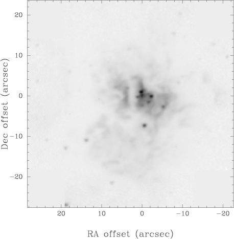
Figure 6: A grey-scale image of the 2.17-$\mu$m Br$\gamma$ plus the continuum. Coordinates of the origin are as in Figure 1.

Figure 7 shows the 2.17-$\mu$m Br$\gamma$ image after the continuum subtraction, which has been Gaussian smoothed to a slightly lower effective spatial resolution of $\sim 0.8$ arcsec. The morphology seen in Figure 7 is strikingly similar to that in the MIR continuum image (see Figure 2, Paper 1). G333.6$-$0.2 has been found to have a blister geometry viewed face-on (Hyland et al. 1980), and the similar morphology exhibited by the ionised gas and warm dust may be accounted for if the MIR emitting dust grains are located behind the H ii region on the front surface of the photo-dissociation region (Paper 1). It is also possible that the gas and dust are well mixed but it is generally thought that dust grains are sublimated at about 1500 K.

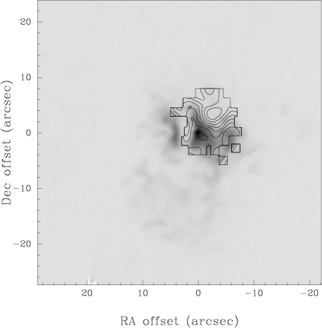
Figure 7: The 2.17-$\mu$m Br$\gamma$ image of G333.6$-$0.2. Grey scale: Same as Figure 6 but after the continuum subtraction and a Gaussian smoothing (see Section 3.2). Contours: Extinction map (see Section 3.2.1). Contours are drawn at $A_{V}=4$ mag interval from 12 mag (near the origin) to 36 mag [near ($-$3,4)].

Table 5 lists the measured Br$\gamma$ fluxes as a function of the aperture sizes and compares the results of the present study to the previously published measurements. Each measurement was made with the aperture centred on the main Br$\gamma$ peak [offset (0,0)] and the overall uncertainty is estimated to be about 5 per cent. The results obtained are consistent with those from the previous studies, especially with the measurements of Wynn-Williams et al. (1978), and imply that the continuum subtraction process was reasonably successful.

Table 5: Measured Br$\gamma$ fluxes (in $\times 10^{-18}$ W cm^-2) as a function of beam size (arcsec).

Beam diameter	Br$\gamma$ flux	Br$\gamma$ flux
	[this study]	[previous studies]
6.0	3.2	2.8a
6.5	3.6	3.5b
30	14	7.3a
32	15	12b

^a Landini et al. (1984); ^b Wynn-Williams et al. (1978)

3.2.1 Extinction map

The theoretical Br$\gamma$ flux (in W cm^-2) is related to the radio flux density $S_{\nu}$ (Jy) measured at frequency $\nu$ (GHz) by

$$F_{{\rm Br}\gamma}=8.90\times 10^{-6}\alpha_{B}\nu^{0.1}\Gamma^{-1}S_{\nu}T_{e}^{0.35},$$

where $\alpha_{B}$ is the total recombination coefficient to the ${\rm n}=2$ level (the ‘on-the-spot’ approximation), and $\Gamma\equiv\frac{N_{{\rm Lyc}}}{N_{{\rm Br}\gamma}}$ is the number ratio of Lyman continuum to Br$\gamma$ photons. $\Gamma$ can be computed for a range of $T_{e}$ and $n_{e}$ using tables of Storey & Hummer (1995).

The observed flux density is related to the theoretical value in the usual way, i.e.,

$$F_{{\rm Br}\gamma}^{{\rm obs}}=F_{{\rm Br}\gamma}^{{\rm theo}}e^{-\tau_{2.17}},$$

where superscripts obs and theo represent observed and theoretical fluxes, respectively, and $\tau_{2.17}$ is the optical depth at the wavelength of the Br$\gamma$ emission. The extinction at a given wavelength $\lambda$ is related to the optical depth by

$$A_{\lambda}=2.5\tau_{\lambda}\log_{10}e.$$

Finally, assuming the extinction at 2.17 $\mu$m, $A_{2.17}\simeq A_{K}$, the extinction found at 2.17 $\mu$m can be extrapolated to the visual extinction at 0.55 $\mu$m using the NIR extinction law derived by Martin & Whittet (1990)

$$A_{K}\simeq 0.09A_{V}.$$

For $T_{e}$, the nearest to the mean value derived earlier (5700 K) in the table of Storey & Hummer (1995), 5000 K was used. The mean value of $n_{e}$ obtained at the same time showed quite a large standard deviation ($\overline{n}_{e}=407000\pm 226000$ cm^-3); however, the 2.17-$\mu$m Br$\gamma$ emission line is not very sensitive to electron densities in the range usually found in H ii regions. Populations of levels are more susceptible to density in high n states, such as those found at radio frequencies, as incoming free electrons have a higher probability of perturbing the bound electrons into a different orbit. Whereas low n transitions [such as Br$\gamma$ (${\rm n}=$ 7$-$4)] are affected less by collisions. We nonetheless used a mean value in the density range $n_{e}=10^{5}-10^{6}$ cm^-3 in the calculation of the theoretical Br$\gamma$ flux.

Some positions exhibit a moderate optical thickness at 3.4 cm (see Table 3). $S_{\nu}$ at each position has therefore been multiplied by a correction factor, [$\tau_{c}/(1-e^{-\tau_{c}})$], which varied from 1.03 at one end of the region mapped with a reasonable $S/N$ (Position 17) to 1.64 at the peak (Position 13). However, the correction can only be made in regions where $\tau_{c}$ is available, i.e., only in the 36 $1.75\times 1.75$-arcsec² boxes. This will confine the extent of the extinction map to the central $\sim 10\times 10$-arcsec².

Landini et al. (1984) measured $A_{V}=18.5$ mag in a 6-arcsec aperture centred on the $K$-band peak. As discussed in Section 2.1.1, radiation from extended structures escaped detection in our current radio interferometric observations. We assumed that the distribution of the missing flux underlying the central compact structure is a 2-D Gaussian. We then adjusted its peak value and FWHMs so that it would contain the amount of the missing flux and contribute sufficient emission in the centre to yield the level of the Landini et al.’s extinction measurement. This was achieved by adding a 2-D Gaussian with a peak value of 0.4 Jy beam^-1 and FWHMs of 20.5 arcsec; however, we note that recently released Spitzer GLIMPSE (Benjamin et al. 2003) images (IRAC 3.6, 4.5, 5.8, & 8.0 $\mu$m) of the G333.6$-$0.2 region show a wide spread ($\sim 2\times 2$ arcmin²), fairly uniform faint emission around more intense (in fact, saturated) central object. Therefore, it is quite possible that there is a large scale pedestal-like extended component to the missing flux, in addition to the 2-D Gaussian structure. If so, the peak value and FWHMs we used for the Gaussian missing flux component are likely to be their respective upper and lower limits. Consequently, our map is more suited to demonstrate the spatial trend in the extinction rather than to show the exact extinction values. It is also noted that, although altering the peak value and FWHMs of the 2-D Gaussian missing flux component changed the finer details of the resultant extinction map, the overall spatial trend remained virtually the same in the central region. Even adding a uniform missing flux produced a very similar trend.

Figure 7 shows the extinction map (contours) superimposed on the Br$\gamma$ image of G333.6$-$0.2. Lower extinction values are found near the Br$\gamma$ peak [offset (0,0)] and in the western extension [around offset ($-$6,$-$1)], i.e., near and around the ionising sources. Point sources with the brightest apparent $K$ magnitudes and the reddest $H-K$ colours were found at these positions, and the large $H-K$ colour excess of those objects most probably indicates the physical association of the point sources with the H ii region (Paper 3). This trend seems to fit with the blister nature of G333.6$-$0.2.

A considerable number of H ii regions have been found to have a blister geometry in which the H ii regions are located at the edges of molecular clouds (Habing & Israel 1979). The blister geometry is thought to be the result of the champagne phase in which H ii regions expand preferentially toward directions of decreasing density (e.g. Yorke 1986). The blister H ii regions are therefore ionisation bounded on the molecular cloud side and density bounded on the side of outward champagne flow (Yorke, Tenorio-Tagle & Bodenheimer 1983). The density of ionized gas decreases approximately exponentially away from the cloud and a large fraction of ionizing photons can escape from the density bounded side. That is, that side can be relatively optically thin. Hyland et al. (1980) found that G333.6$-$0.2 is a blister H ii region viewed face-on. The density bounded side then is the front face and the low extinction values found around the ionizing sources are perhaps natural consequences of this geometry.

Taken at face value, the presence of red objects in lower extinction regions may seem contradictory; however, it was shown in Paper 3 that, in the colour-colour diagram space, for example, these red sources are found significantly away from the average interstellar extinction curves. It was also demonstrated that emission from hot ($\gtrsim 600$ K) dust grains, which are likely to be located in circumstellar discs, is considerably more important in the $K$-band than at $H$, resulting in the large $H-K$ colours of these objects. In other words, the red colours are due not to the extinction but to the intrinsic infrared excess, and so it is not implausible for these sources to be found in lower extinction regions.

There is a slight increase in extinction between the main and secondary peaks. In a clumpy medium, an expansion front (weak ionisation front with its associated shock) of an H ii region passes around the more dense clumps of neutral material and compresses them (Yorke 1986), which results in embedded neutral globules and dark lanes sometimes seen in optical images of emission nebulae. As mentioned earlier, there is likely to be an ionizing source both in the main and secondary peaks and the gap between the two peaks observed at NIR and MIR wavelengths could be a pressure compressed dense region that consequently shows a high extinction, rather than a foreground extinction lane. The fact that this gap is also observed at radio frequencies (see Figures 1 & 2) may support this suggestion.

The highest extinction is located near offset ($-$3,4). It was suggested in Paper 2 that there is likely to be an extra overlapping of dense, cold material containing silicates at 5 arcsec north of the main MIR peak, since the spectrum taken at the position showed a deep silicate absorption. The beam size used for the 5$.\!\!^{\prime\prime}$0N position was 5.6 arcsec in diameter and most likely included this region of high extinction. The position coincides with a radio peak (see Section 3.3) and the high extinction may be associated with this radio source.

3.2.2 The Lyman continuum photons

The theoretical Br$\gamma$ flux can also be expressed as

$$F_{{\rm Br}\gamma}^{{\rm theo}}=\frac{N_{{\rm Br}\gamma}}{4\pi D^{2}}\ \frac{hc}{\lambda_{{\rm Br}\gamma}},$$

where $D$ is the distance to the object (in cm), $h$ is the Planck’s constant, and $\lambda_{{\rm Br}\gamma}$ is the wavelength of the Br$\gamma$ emission. And recalling that $\Gamma\equiv\frac{N_{{\rm Lyc}}}{N_{{\rm Br}\gamma}}$,

$$N_{{\rm Lyc}}=4\pi D^{2}\frac{\lambda_{{\rm Br}\gamma}}{hc}F_{{\rm Br}\gamma}^{{\rm theo}}\Gamma.$$

Again by knowing $S_{\nu}$, $n_{e}$ and $T_{e}$, and using an appropriate table from Storey & Hummer (1995), the number of Lyman continuum photons can be estimated.

In constructing the extinction map, we have assumed a 2-D Gaussian-shaped missing flux distribution. This also means that the missing flux is concentrated and that $\sim 100$ per cent of the total flux at 3.4 cm (80 Jy, McGee et al. 1975) comes from the inner region. However, such a high concentration of flux in the centre is most probably the upper limit as there appears to be a wider spread of faint emission further out (see above). The number of Lyman continuum photons in the inner $\sim 50$-arcsec is thus estimated to be $\lesssim 9.5\times 10^{49}$ s^-1.

Rubin et al. (1994) suggested that the effective temperature ($T_{{\rm eff}}$) of star(s) exciting G333.6$-$0.2 is $\sim 36000$ K which, according to the stellar spectral-type scale of Martins, Schaerer & Hillier (2005), is approximately characteristic of an O7V star. The number of the Lyman continuum photons emitted by an O7V star is estimated to be $\sim 5\times 10^{48}$ s^-1 (Martins et al. 2005). Therefore, if all the exciting stars in G333.6$-$0.2 were of the same spectral type, there would be up to 19 O7V stars. In Paper 1, it was found that about a dozen O8V stars ($T_{{\rm eff}}=36000$ K) is required to radiate the ionising photon flux necessary to produce the observed [Ne ii] central dip.

3.3 Velocity structure (revisited)

The double peak of an RRL observed in an H ii region could be interpreted as:

(a) expansion of shell-like structure,

(b) rotation,

(c) two H ii regions at different velocities, or,

(d) outflows/jets.

We discuss each of these in turn, followed by a short section (e), describing details of a toy model for our preferred option, (d).

(a) expansion of shell-like structure. There is no obvious shell-like morphology seen in the regions where double peaks are observed. The mean velocity difference between the two lines is $\sim 30$ km s^-1. For a shell-like structure to be unresolved ($<1.6$ arcsec or $<0.023$ pc) and to have an expansion velocity of $\sim 30$ km s^-1 would require a dynamical age of only a few hundred years. This seems rather unlikely. Also, the stellar-wind blown cavity scenario for the [Ne ii] central dip was ruled out in Paper 1, since there were no signs of such a cavity in the continuum image at a nearby wavelength.

(b) rotation. This appears unlikely since there is no systematic shift of central velocities across the region to suggest a rotation.

(c) two H ii regions at different velocities. Combined with the multiple point sources seen in the NIR images (see Figure 6 and Paper 3), it could be that the double peak profiles of the H90$\alpha$ RRL in G333.6$-$0.2 represent the existence of several compact H ii regions at different velocities. In the $JHK^{\prime}$ images (Paper 3), all of which were taken at a similar spatial resolution to that of the radio maps presented here, at least four point sources were identified in the central region of G333.6$-$0.2, two of which are found in the main peak (cf. NM and SM in Figure 7, Paper 3), one in the secondary peak to the east of the main, and one in the south-west extension. Double peak regions do indeed coincide with the MIR main peak and the south-west extension. At the highest spatial resolution so far attained ($\sim 0.6$ arcsec), the 2.17-$\mu$m image (Figure 6) reveals even more star-like point sources in the central region and there appears to be three sources located very close together near the position of the MIR main peak.

Figure 8 shows intensity distribution in each velocity plane ($\sim 4$ km s^-1 wide) in the range $\sim-100$ to $0$ km s^-1. This sequence of velocity maps also reveals the multiple nature of the exciting source in the central region of G333.6$-$0.2. The main radio peak dominates throughout the velocity range because of its large line width ($\sim 50$ km s^-1 FWHM). The ridge to the south of the main peak is visible up to the $-62$ km s^-1 frame but is absent till another peak appears further south at about $-50$ km s^-1. The south-west extension seems to contain at least three peaks (see also Figures 1 & 2). As mentioned earlier, there is at least one point source identified in the NIR images in the south-west extension (see Figure 6 and Paper 3).

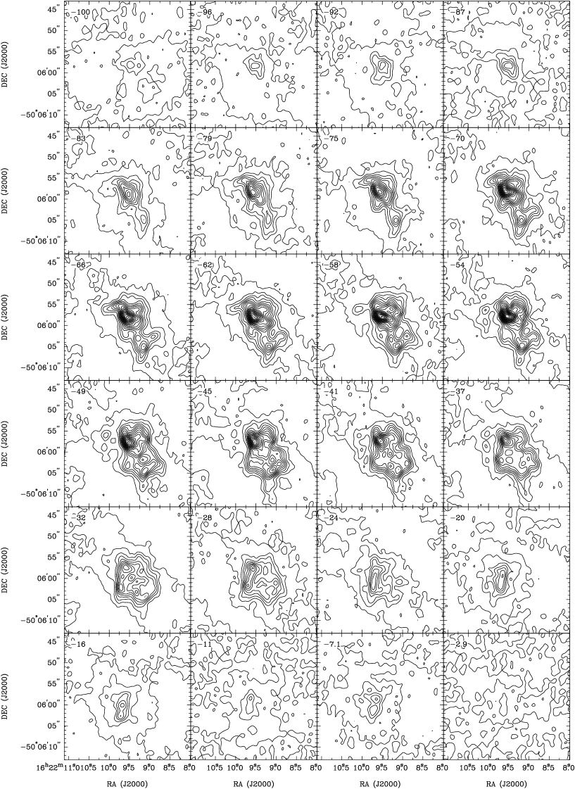
Figure 8: The H90$\alpha$ RRL maps in each velocity plane ($\sim 4$ km s^-1 wide). The velocity plane is indicated at the top left hand corner of each plot. The contours are drawn at a 5 per cent interval from 0 to 100 per cent of the maximum flux density in each plane. The maximum values in each plane are 1.4, 1.8, 2.2, 2.3, 3.8, 5.0, 5.8, 8.1, 8.0, 8.3, 8.4, 9.2, 7.5, 6.9, 6.0, 5.3, 4.0, 3.7, 3.2, 2.8, 2.5, 1.5, 1.9, and 0.82 $\times 10^{-2}$ Jy beam^-1 from $-100$ to $-2.9$ km s^-1.

The shape of the radio main peak is rather complex. There appears to be another peak close (about 2 arcsec north-west) to the main peak (see the $-$58 km s^-1 frame). The extinction map (Figure 7) shows a large increase in the extinction value around this position, which may imply that obscuring dust grains are associated with this peak. The main peak and this nearby local maximum do not have obvious IR counterparts and could be younger than the other exciting sources in the H ii region, which in turn may also explain the presence of heavy obscuring dust grains. If this supposition of the difference in age were correct then this alone would lead to the conclusion of multiple exciting sources, and hence the presence of several compact H ii regions, in G333.6$-$0.2.

If flat Galactic rotation curves, with a constant circular velocity $\Theta=220$ km s^-1 and the Sun’s distance from the Galactic centre $R_{0}=8.5$ kpc, were adopted, the difference in velocity of $\sim 30$ km s^-1 between two peaks in the double peak regions would imply a separation of the H ii regions along the line of sight (los) of $\sim 1.6$ kpc. While possible, it seems rather unlikely that several unassociated compact H ii regions just happen to coincide along the los to produce the velocity structure observed. Of course, G333.6$-$0.2 is an active star-forming complex and adopting the Galactic rotation curves to interpret the velocity structure may not be appropriate.

Another interesting feature that is difficult to interpret with the los coincidence scenario for the complex velocity structure presents itself when the single and double peak spectra are compared closely. Figure 9 shows the best-fit Gaussian profiles at Positions 13, 14, and 15. It is remarkable that the overall shape of the spectra matches almost exactly and the double peak appears more or less symmetric with the single peak between the two peaks. Again it seems rather unsatisfactory to explain such features as a chance coincidence of compact H ii regions along the los.

Figure 9: Gaussian profiles at Positions 13, 14, and 15 (see also Figure 5).

The spatial resolution of the radio maps (1.6 arcsec), despite being the highest so far obtained at these frequencies and for the first time revealing the double peak profile of the H90$\alpha$ RRL, is more than twice the highest resolution of the IR images ($\sim 0.6$ arcsec). To examine more closely the relationship between the IR point sources and the velocity structure, radio interferometric observations at even higher spatial resolution, at least that comparable to the IR images, are required. IR imaging both at high spectral and spatial resolution is perhaps an alternative.

(d) outflow or jets. There are no obvious structures that suggest outflows or jets in the double peak regions. However, it is possible that outflows/jets are inclined in the los so that such structures are not immediately obvious, or are unresolved by the 1.6-arcsec beam. Yorke et al. (1983) produced theoretical radio continuum maps of H ii regions in the champagne phase, which occurs when the ionisation front of an H ii region encounters a region of strong density gradients, such as the boundary of a molecular cloud. They found that the champagne outflow (or preferential expansion of an H ii region along negative density gradients) can attain high velocity ($>10$ km s^-1) and in the case of a slab-like geometry it can be bipolar. They also found that in general the maximum of radio emission, which is proportional to $n_{e}^{2}$ (e.g. Rubin 1968), does not coincide with the ionizing source. This may explain the offset between the radio and IR sources.

The champagne outflow scenario may also explain the broad line width of the single peak. The outflows caused by the preferential expansion of the H ii region into less dense regions may not be well-collimated. In fact, the velocity structure depicted in the models of Yorke et al. (1983) shows a fan-like radial outpouring of ionized gas from the mouth of the outflow. If an RRL were observed from such a structure its spectrum would probably show a large line width due to a range of los velocities present in the radial velocity field.

It was found in Paper 2 that the intrinsic magnetic field lines follow well the flux distribution north-west of the MIR main peak. This morphology is most likely to be due to the presence of a clump of dense material containing silicates (indicated by the shape of the spectrum taken at 5 arcsec north of the MIR main peak). There is a local visual extinction maximum about 4 arcsec north and 3 arcsec west of the IR main peak (Figure 7), which may be associated with the radio peak $\sim 2$ arcsec north and $\sim 3$ arcsec west of the radio main peak seen in the $-58$ km s^-1 plane (see Figure 8). The expanding H ii region may have carried the frozen-in, threading magnetic field with its expansion. If such structure then encountered the aforementioned clump of dust and compressed the magnetic field against it the intrinsic polarization pattern may result. Near the boundary, where the expansion hit the clump, the radio continuum peak may have been produced by the high density.

(e) a toy model. In view of the ability of the outflow model to account for the general appearance, we present (Figure 10) a more elaborate toy model of G333.6$-$0.2, which can explain all of the key features. The blister geometry, that may account for the trend found in the extinction map (Figure 7), may not be exactly face-on but somewhat tilted south-east. Towards the north of the exciting (IR) source(s), as we look through a range of los velocities in the fanned-out champagne outflow in the relatively high density regions near the molecular cloud wall, we observe the strong, broad single RRL (los 1, Figure 10). We obtain double RRL spectra towards the south-east, as faster flows are found along the wide opening of the blister ‘bowl’, whilst flows in the intermediate velocity range are generally fainter (as the region is more diffuse) and relatively perpendicular with respect to the los (los 2, Figure 10). Champagne flow velocities are expected to be greater further away from the molecular cloud (Bedijn & Tenorio-Tagle 1981) and we are possibly observing this phenomenon as there seems to be an apparent trend that the blue peak shifts to the bluer velocity (and the red redder) the more south we look (see Table 4).

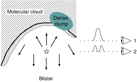
Figure 10: A ‘cartoon’ representation (a side view) of a possible situation in G333.6$-$0.2. ✩ denotes the IR exciting source(s). Two different lines of sight (1 and 2) are also indicated, together with a probable RRL profile along each los. Arrows are drawn only to illustrate likely direction of the champagne flows. See text for details.

Another interesting feature, which may be explained by this picture, is that in the north the blue peak is stronger, whereas the red peak becomes brighter in the south (see Figures 4, 5, and 9). This could be due to the presence of the dense clump. The density near the front side of the molecular cloud wall is enhanced by the dense clump and therefore, near the clump, we find strongest emission from the flows that are directed towards us; south of the clump, emission from the back wall (away from us) dominates. Note that, whilst the strength of the blue peak changes dramatically depending on the exact position, the red peak brightness remains more or less constant.

4 Conclusions

The radio interferometric observations and NIR imaging of the southern massive star-forming region G333.6$-$0.2 are presented. The morphologies of the high spatial resolution (1.6-arcsec) 3.4-cm continuum and H90$\alpha$ RRL maps are remarkably similar to each other and to the IR images. However, the radio main peak neither coincides with the IR main peak nor has any obvious IR counterparts. The H90$\alpha$ RRL spectra show a complex structure with a double peak profile at some positions observed for the first time. The complex velocity structure may be explained by champagne outflows, which may also explain the offset between the radio and IR sources. The 3.4-cm radio continuum map is combined with the 2.17-$\mu$m Br$\gamma$ image in constructing the visual extinction map. The blister geometry of the H ii region probably causes the trend seen in the extinction map. The number of Lyman continuum photons in the central 50-arcsec is estimated to be equivalent to that emitted by $\lesssim 19$ O7V stars.

References

- Aitken et al. (1977) Aitken D. K., Griffith J., Jones B., 1977, MNRAS, 179, 179
- Allen et al. (1993) Allen D. A., et al., 1993, PASAu, 10, 298
- Bedijn & Tenorio-Tagle (1981) Bedijn P. J., Tenorio-Tagle G., 1981, A&A, 98, 85
- Benjamin et al. (2003) Benjamin R. A., et al., 2003, PASP, 115, 953
- Brocklehurst & Salem (1977) Brocklehurst M., Salem M., 1977, Comp. Phys. Comm., 13, 39
- Brown (1987) Brown R. L., 1987, in Dalgarno A., Layzer D., eds, Spectroscopy of astrophysical plasmas, Cambridge University Press, p.35
- Burton (1992) Burton M. G., 1992, AuJPh, 45, 463
- Carter & Meadows (1995) Carter B. S., Meadows V. S., 1995, MNRAS, 276, 734
- Caswell & Haynes (1987) Caswell J. L., Haynes R. F., 1987, A&A, 171, 261
- Colgan et al. (1993) Colgan S. W. J., Haas M. R., Erickson E. F., Rubin R. H., Simpson J. P., Russell R. W., 1993, ApJ, 413, 237
- Esteban et al. (1999) Esteban C., Peimbert M., Torres-Peimbert S., García-Rojas J., Rodríguez, M., 1999, ApJS, 120, 113
- Ferland (2001) Ferland G. J., 2001, PASP, 113, 41
- Fujiyoshi et al. (1998) Fujiyoshi T., Smith C. H., Moore T. J. T., Aitken D. K., Roche P. F., Quinn D. E., 1998, MNRAS, 296, 225 (Paper 1)
- Fujiyoshi et al. (2001) Fujiyoshi T., Smith C. H., Wright C. M., Moore T. J. T., Aitken D. K., Roche P. F., 2001, MNRAS, 327, 233 (Paper 2)
- Fujiyoshi et al. (2005) Fujiyoshi T., Smith C. H., Moore T. J. T., Lumsden S. L., Aitken D. K., Roche P. F., 2005, MNRAS, 356, 801 (Paper 3)
- Goss & Shaver (1970) Goss W. M., Shaver P. A., 1970, AuJPA, 14, 1
- Habing & Israel (1979) Habing H. J., Israel F. P., 1979, ARA&A, 17, 345
- Hyland et al. (1980) Hyland A. R., McGregor P. J., Robinson G., Thomas J. A., Becklin E. E., Gatley I., Werner M. W., 1980, ApJ, 241, 709
- Kingdon & Ferland (1995) Kingdon J. B., Ferland G. J., 1995, ApJ, 450, 691
- Landini et al. (1984) Landini M., Natta A., Oliva E., Salinari P., Moorwood A. F. M., 1984, A&A, 134, 284
- McGee & Newton (1981) McGee R. X., Newton L. M., 1981, MNRAS, 196, 889
- McGee et al. (1975) McGee R. X., Newton L. M., Batchelor R. A., 1975, AuJPh, 28, 185
- Martin & Whittet (1990) Martin P. G., Whittet D. C. B., 1990, ApJ, 357, 113
- Martins et al. (2005) Martins F., Schaerer D., Hillier D. J., 2005, A&A, 436, 1049
- Moneti & Moorwood (1989) Moneti A., Moorwood A. F. M., 1989, in Infrared spectroscopy in astronomy, ESA, p.299
- O’dell et al. (2003) O’Dell C. R., Peimbert M., Peimbert A., 2003, AJ, 125, 2590
- Roelfsema & Goss (1992) Roelfsema P. R., Goss W. M., 1992, A&ARv, 4, 161
- Roelfsema et al. (1992) Roelfsema P. R., Goss W. M., Mallik D. C. V., 1992, ApJ, 394, 188
- Rubin (1968) Rubin R. H., 1968, ApJ, 154, 391
- Rubin et al. (1994) Rubin R. H., Simpson J. P., Lord S. D., Colgan S. W. J., Erickson E. F., Haas M. R., 1994, ApJ, 420, 772
- Shaver et al. (1983) Shaver P. A., McGee R. X., Newton L. M., Danks A. C., Pottasch S. R., 1983, MNRAS, 204, 53
- Storey & Hummer (1995) Storey P. J., Hummer D. G., 1995, MNRAS, 272, 41
- Wood & Churchwell (1989) Wood D. O. S., Churchwell E., 1989, ApJS, 69, 831
- Wynn-Williams et al. (1978) Wynn-Williams C. G., Becklin E. E., Matthews K., Neugebauer G., 1978, MNRAS, 183, 237
- Yorke (1986) Yorke H. W., 1986, ARA&A, 24, 49
- Yorke et al. (1983) Yorke H. W., Tenorio-Tagle G., Bodenheimer P., 1983, A&A, 127, 313