The 3D skeleton of the SDSS

Abstract

The length of the three-dimensional filaments observed in the fourth public data-release of the SDSS is measured using the local skeleton method. It consists in defining the set of points where the gradient of the smoothed density field is extremal along its isocontours, with some additional constraints on local curvature to probe actual ridges in the galaxy distribution. A good fit to the mean filament length per unit volume, $\cal{L}$, in the SDSS survey is found to be ${\cal{L}}=(52500\pm 6500)\,(L/{\rm Mpc})^{-1.75\pm 0.06}\rm{Mpc}/(100\,\rm{Mpc})^{3}$ for $8.2\leq L\leq 16.4$ Mpc, where $L$ is the smoothing length in Mpc. This result, which deviates only slightly, as expected, from the trivial behavior ${\cal{L}}\propto L^{-2}$, is in excellent agreement with a $\Lambda$CDM cosmology, as long as the matter density parameter remains in the range $0.25<\Omega_{\rm matter}<0.4$ at one sigma confidence level, considering the universe is flat. These measurements, which are in fact dominated by linear dynamics, are not significantly sensitive to observational biases such as redshift distortion, edge effects, incompleteness, and biasing between the galaxy distribution and the dark matter distribution. Hence it is argued that the local skeleton is a rather promising and discriminating tool for the analysis of filamentary structures in three-dimensional galaxy surveys.

1. Introduction

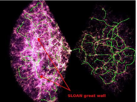
Figure 1.— Derived 3D skeleton in a slice of the SDSS for a smoothing length $L=16.4$ Mpc. This animation still frame shows how well structures are captured, notably the SLOAN great wall. The mpeg movie version is available at http://www.projet-horizon.fr/article173.html.

From the Great Wall of CFA1 (Geller & Huchra, 1989) to the very long filaments seen in the SDSS (Gott et al., 2005) and the 2DF (Colless et al., 2001), the ever growing size of the largest structures observed in the three-dimensional galaxy distribution has remained a challenge to models of large scale structure formation. It is therefore of prime importance to find a robust way to identify filaments in the Universe and to characterize them, e.g. through their length, thickness and/or average density. To achieve that, one usually relies on the analysis of the morphological properties –e.g. through structure functions (Babul & Starkman, 1992), Minkowski functionals (Mecke et al., 1994), shape finders (Sahni et al., 1998)– of an excursion’s connected components in overdense regions of the catalog, which can be obtained using friend-of-friend algorithms (Zel’dovich et al., 1982), the minimum spanning tree technique (Barrow et al., 1985; Doroshkevich et al., 2004) or percolation on a grid where the density field has been smoothly interpolated (Gott et al., 86; Dominik & Shandarin, 1992).

This letter works instead in the framework of Morse theory (Colombi et al., 2000), and uses the approach proposed recently by Novikov et al. (2006, hereafter NCD) and Sousbie et al. (2006, hereafter SPCN), where filaments are seen as a set of special field lines, departing from saddle points and converging to local maxima while following the gradient of the density field, $\nabla\rho\equiv\partial\rho/\partial x_{i}\equiv\rho_{i}$. However, the skeleton thus defined remains non-local, which makes analytical calculations challenging and edge effects difficult to cope with in real catalogs. To solve these issues, a local approximation of the skeleton was proposed by NCD in the 2D case, and generalized to 3D by SPCN. Given the Hessian, ${\cal H}\equiv\partial^{2}\rho/\partial x_{i}\partial x_{j}\equiv\rho_{ij}$, and its eigenvalues, $\lambda_{i}$, ranked in decreasing order, the local skeleton is defined as the set of points where ${\cal H}\cdot\nabla\rho=\lambda_{1}\nabla\rho$ and $\lambda_{2},\lambda_{3}<0$, to ensure that ridges of the density field are probed.

In this paper, the local skeleton is extracted from the SDSS DR4 galaxy catalog. Its total length per unit volume is measured and compared to that obtained in $\Lambda$CDM cosmologies. Relying on realistic mock catalogs, various effects such as incompleteness, survey geometry, cosmic variance, redshift distortions, biasing and non-linear dynamics, are extensively tested.

Table 1Length per unit volume of the skeleton for different SDSS and mock samples

	L	DR4-350	DR4-VL350	MOCK	MOCK-PS	MOCK-AS	MOCK-NB
length density	16.4	372	363	390 $\pm$ 19	395$\pm$ 16	362	403 $\pm$ 17
$[\rm{Mpc}/(100\,\rm{Mpc})^{3}]$	10.9	795	772	796 $\pm$ 18	815$\pm$ 19	740	790 $\pm$ 24
	8.2	1271	1299	1272 $\pm$ 25	1308$\pm$ 27	1285	1204 $\pm$ 25

2. Observational and mock data samples

A complete description of the Fourth Data Release of the Sloan Digital Sky Survey (DR4 SDSS) can be found in Adelman-McCarthy et al. (2006). The main sample used in this paper is extracted from the Catalog Archive Server facility. To ensure proper spectral identification of galaxies, objects with specclass $=2$ and zconf $>0.35$ are selected in the specphoto table. This yields a main sample containing $459,408$ galaxies. The completeness in apparent magnitude was investigated and is achieved for $U_{\rm{SDSS}}<19$. Two subsamples were extracted: a sample cut at distance $d<350$ Mpc containing $148,012$ galaxies (hereafter DR4-350), and a homogeneous, volume-limited sample (hereafter DR4-VL350) containing $25,843$ galaxies selected on the basis of their absolute magnitude $M_{\rm absU}<-17$ and $d<350$ Mpc.

To test the robustness of the measurements and compare observational results to theoretical predictions, a large $\Lambda$CDM simulation was performed, using the publicly available treecode GADGET-2 (Springel, 2005), involving $512^{3}$ particles in a $1024\,h^{-1}\rm{Mpc}$ box, and with the following cosmological parameters: $H_{0}=70$ km/s/Mpc, $\Omega_{\rm baryons}=0.05$, $\Omega_{\rm matter}=0.3$, $\Omega_{\Lambda}=0.7$ and normalization $\sigma_{8}=0.92$. Various mock catalogs were extracted from this simulation, using MoLUSC (Sousbie et al. 2006b, ). This tool is designed to build realistic mock galaxy catalogs from dark matter simulations of large volume but poor mass resolution, by reprojecting, as functions of local phase-space density, the statistical properties of the galaxy distribution (type, spectral features, number density, etc.) derived from semi-analytic models applied to simulations of higher mass resolution. Here, the results calculated by GalICS (Hatton et al., 2003) on a treecode simulation with $256^{3}$ particles in a cube of $150$ Mpc on a side are used as inputs of MoLUSC. According to the analyses of Blaizot et al. (2006), this simulation should provide sufficient mass resolution to describe realistically the statistical properties of SDSS galaxies with $U_{\rm{SDSS}}<19$. The advantage of using MoLUSC is that it allows one to probe a realistic volume of the Universe without worrying about finite volume or replication effects in the realization of mock catalogs themselves (Blaizot et al., 2005).

For the purpose of testing the skeleton properties, three different kinds of mock catalogs were built, all cut at a distance of $350$ Mpc: (1) the main catalog is called MOCK and attempts to reproduce all the characteristics of DR4-350 (redshift space distortion, incompleteness, survey geometry, etc.); (2) MOCK-PS is identical to MOCK but uses the exact positions of the galaxies to test the effect of redshift distortion; (3) MOCK-AS is an all-sky version of MOCK aimed to test the influence of survey geometry and finally (4) MOCK-NB is identical to MOCK but with dark matter particles (without density biasing). The volume of our simulation is approximately 30 times that covered by DR4-350, which yields an error bar reflecting cosmic variance from the dispersion among 25 random realizations of MOCK. Note finally that measurements were also performed directly on the dark matter distribution simulation boxes and on the initial conditions of the simulation, to test the effects of nonlinear clustering.

3. The 3D Skeleton: algorithm

The details of the algorithm used to draw the local skeleton defined in § 1 are given in SPCN, so only a brief sketch of it is given here:

(i) interpolation and smoothing: the first step consists in performing cloud-in-cell interpolation (Hockney & Eastwood, 1981) on a $512^{3}$ grid covering a $700$ Mpc cube embedding the survey. To avoid extra degeneracies while drawing the skeleton, the empty regions of the cube are filled with a random distribution of galaxies with $1,000$ times smaller average density than inside the survey. At the end of the process, only the parts of the skeleton belonging to the original survey are kept. To warrant sufficient differentiability, convolution with a Gaussian window of size $L$ is performed prior to computing the gradient and the Hessian using a finite difference method. As argued in NCD, in order to avoid contamination by the grid, discreteness and finite volume effects, respectively, the smoothing scale should verify $L/\Delta\lower 2.15277pt\hbox{$\;\buildrel>\over{\sim}\;$}4$, $L/\lambda\lower 2.15277pt\hbox{$\;\buildrel>\over{\sim}\;$}1$ and $L/V^{1/3}\lower 2.15277pt\hbox{$\;\buildrel<\over{\sim}\;$}20$ where $\Delta$ is the grid step, $\lambda$ the mean interparticle distance and $V$ is the survey volume. As a result, the following conservative scale range, $8.2\leq L\leq 16.4$ Mpc, will be used for the measurements performed in this paper.

(ii) surface intersection modeling: the second step of the algorithm consists in drawing the skeleton, noting that it is embedded in the set of points verifying ${\cal H}\cdot\nabla\rho\times\nabla\rho=0$. This leads to 3 conditions, $S_{i}(x_{1},x_{2},x_{3})=0$, that define 3 surfaces intersecting along a common line. The actual method used to compute the surfaces $S_{i}=0$ as an assemblage of triangles and their intersections as a set of connected lines relies on the classical marching cube algorithm (Lorensen & Cline, 1987), as detailed further in SPCN. Additional conditions, namely that the gradient should be aligned with the major axis of curvature – in practice, $|\nabla\rho.{\bf u}_{1}|>\rm{max}\left(|\nabla\rho.{\bf u}_{2}|,|\nabla\rho.{\bf u}_{3}|\right)$ where ${\bf u}_{i}$ are the eigenvectors of ${\cal H}$– and $\lambda_{2},\lambda_{3}<0$ are enforced locally after diagonalizing the Hessian.

(iii) cleaning: some additional treatment has to be performed in regions where the field becomes degenerate (e.g. in the vicinity of critical points, $\nabla\rho=0$), as explained in detail in SPCN. Finally, the parts of the local skeleton which do not pass through any critical point are removed. As argued in SPCN, these parts are mostly irrelevant as they do not, in general, correspond to real filaments.

4. Measurements and robustness vs observational biases

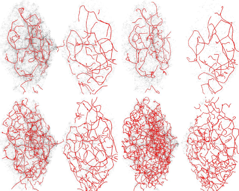
Figure 2.— The skeleton of the SDSS compared to the corresponding galaxy distribution. Top left and right panels: the galaxy distribution, respectively in DR4-350 and its volume-limited counterpart, DR4-VL350 with the superimposed skeleton measured for a smoothing scale $L=16.4$ Mpc. Bottom left and right panels: the skeleton measured in DR4-350, for $L=10.9$ and $8.2$ Mpc, respectively. To have a better feeling of what the results look like in 3D, a mpeg movie is also available in the electronic edition of the Astrophysical Journal, where the skeleton is measured on the full SSDS-DR4 data for $L=16.4$ Mpc.

Figure 2 shows the skeleton measured in DR4-350 for 3 smoothing scales $L=16.4$, $10.9$ and $8.2$ Mpc, (top left and 2 bottom panels) while the measurements of its length, ${\cal L}$ as a function of $L$ are summarized in Table 1.

As expected, the skeleton matches the intuitive visual definition of what a filament is, and its length and complexity increase with the inverse of $L$. Notice on Fig. 2 that the prominent features of the skeleton remain mostly independent of smoothing: decreasing $L$ essentially adds new branches to the skeleton, corresponding to finer structures in the galaxy distribution. In other words, the skeleton grows like a tree, while $L$ decreases. The overall scale dependence of the measured length, ${\cal{L}}=(52500\pm 6500)(L/{\rm Mpc})^{-1.75\pm 0.06}\rm{Mpc}/(100\,\rm{Mpc})^{3}$, is in good qualitative agreement with the expected trivial power-law in the scale-free case, ${\cal L}\propto L^{-2}$ (SPCN).

These results match very well the predictions of the standard $\Lambda$CDM model (compare MOCK to DR4-350). This allows one to use the mock catalogs as a solid baseline to test possible observational and dynamical effects on the skeleton, as discussed now, using Table 1 as a guideline. Incompleteness and discreteness effects can simultaneously be tested by comparing DR4-350 to its volume-limited counterpart, DR4-VL350, which probes only 15 percent of the galaxies available in DR4-350 (see the top panels of Fig. 2). They have little impact on the skeleton, changing its length by at most 3 percent. Edge effects arise from the particular geometry of the SDSS. They can be probed by comparing MOCK to MOCK-AS. They have a small but systematic impact on the measured length of the skeleton, which is increasingly overestimated with scale, from about 1 percent for $L=8.2$ Mpc to 8 percent for $L=16.4$ Mpc. In terms of scaling behavior, ${\cal L}\propto L^{-\alpha}$, $\alpha$ is therefore slightly underestimated, which explains partly the slight deviation from the expectation $\alpha=2$, in addition to the scale dependence of the power-spectrum of the density fluctuations. Cosmic variance should be small: when estimated from the dispersion among 25 realizations of MOCK, it increases with smoothing scale, as expected, from a 2 percent error for $L=8.2$ and $L=10.9$ to a $5$ percent error for $L=16.4$. Redshift distortion effects, discussed at length in SPCN, can be tested by comparing MOCK to MOCK-PS. They have negligible impact on the measurements, well within the cosmic variance. Finally, since the skeleton probes overdense regions of the universe and large smoothing scales are considered, the measurements are expected to be rather insensitive to effects of biasing and to be dominated by the predictions of linear dynamics. This has been fully confirmed when comparing the skeleton of simulations at $z=0$ and in the initial conditions, at least in the $\Lambda$CDM cosmogony framework. Moreover, the small amplitude of the change of length of the skeleton when nonlinear biasing is applied can be checked in Table 1 (compare MOCK-NB and MOCK).

5. Discussion: a test of LSS formation models

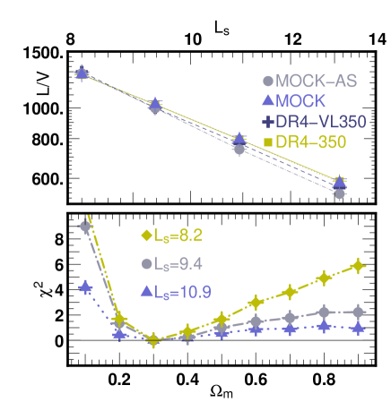
Figure 3.— Top panel: skeleton length per unit volume (in Mpc$/$($100$ Mpc)³) as a function of smoothing length for mock catalogs and SDSS showing the very good agreement (as explained in the text). The error bars correspond to the cosmic variance, which is estimated via 25 realizations of the mock. Bottom panel: $\chi^{2}$ corresponding to the squared difference between the total length per unit volume of the mock catalog and that of the SDSS, in units of the RMS of the mock; These $\chi^{2}$ curves yield a confidence interval for $\Omega_{\rm matter}$ (for a flat universe) of $[0.25,0.4]$ at one-$\sigma$ level and $[0.15,0.75]$ at two-$\sigma$ level. The simulations are $256^{3}$ dark matter particles of a given $H_{0}=70$ km/s/Mpc using an Eke prescription (Eke et al., 1996) for the normalization of the spectrum.

In this letter a method to probe the filamentary structure in the galaxy distribution, involving the extraction of the local skeleton from the data and measuring its length per unit volume, ${\cal L}$, was tested on the SDSS and mock catalogs. The length of the skeleton was found to be a robust statistic in the scaling regime $8.2\leq L\leq 16.4$ Mpc, rather insensitive to nonlinearities, biasing, redshift distortion, incompleteness and cosmic variance. The results were however slightly affected by edge effects due to the geometry of the SDSS (see Table 1 Column 6). Still, one observes an excellent agreement with the $\Lambda$CDM concordant model. (See figure 3, top panel).

One question remains: is the length of the skeleton a discriminant measure of large scale structure? In theory, the answer is positive: for a Gaussian field, ${\cal L}$ depends on the shape of the power-spectrum of density fluctuations, $P(k)$, through its moments of order $2m$, $\int k^{2m+2}P(k)\exp(-k^{2}L^{2}){\rm d}k$, up to $m=3$, leading to the approximate scaling ${\cal L}\propto(6.2+n)L^{-2}$ for $P(k)\propto k^{n}$ (SPCN). To demonstrate that this spectral dependence can be used to constrain models of large scale structure in practice, nine flat universe simulations were carried out with GADGET-2, involving $256^{3}$ particles and with the same cosmological parameters as previously used except that $\Omega_{\rm matter}$ was left as a free variable in the range $0.1\leq\Omega_{\rm matter}\leq 0.9$. From each of the simulations, 25 mock catalogs were extracted, in which ${\cal L}$ was estimated. These measurements were used to perform standard $\chi^{2}$ analysis to find the best matching value of $\Omega_{\rm matter}$ for the SDSS, using MOCK as reference. The final $1\sigma$ constraint is $0.25<\Omega_{\rm matter}<0.4$ (See figure 3).

This clearly demonstrates that the length of the skeleton is a discriminant estimator,

which might prove to be a real alternative to traditional two-point statistics estimators which are extremely sensitive to the bias in the nonlinear stage of gravitational instability. The local skeleton extraction also opens new paths of investigation for the structure analysis of galactic or dark matter distribution, with the prospect of defining quantitatively the locus of filaments. In particular, it will allow astronomers to carry measurements (velocity, pressure…) along the main motorways of galactic infall (Aubert et al., 2004).

References

- Adelman-McCarthy et al. (2006) Adelman-McCarthy, J. K., et al. , 2006, ApJS 162, 38
- Aubert et al. (2004) Aubert, D., Pichon, C., Colombi, S. 2004, MNRAS, 352, 376
- Babul & Starkman (1992) Babul, A., Starkman, G. D., 1992, ApJ 401, 28
- Barrow et al. (1985) Barrow, J. D., Bhavsar, S. P., Sonoda, D. H., 1985, MNRAS 216, 17
- Blaizot et al. (2005) Blaizot, J. et al. , 2005, MNRAS360, 159
- Blaizot et al. (2006) Blaizot, J., et al. 2006, MNRAS, in press
- Colless et al. (2001) Colless, M., et al., 2001, MNRAS, 328, 1039
- Colombi et al. (2000) Colombi, S., Pogosyan, D., Souradeep, T., 2000, Phys. Rev. Lett. 85, 5515
- Dominik & Shandarin (1992) Dominik, K. G., Shandarin, S. F., 1992, ApJ 393, 450
- Doroshkevich et al. (2004) Doroshkevich, A., Tucker, D. L., Allam, S., Way, M. J., 2004 A&A 418, 7
- Eke et al. (1996) Eke, V. R., Cole, S., & Frenk, C. S. 1996, MNRAS, 282, 263
- Fukugita (2004) Fukugita, M., et al, 2004 AJ 127,
- Geller & Huchra (1989) Geller, M.J., Huchra, J.P. 1989, Science, 246, 897
- Gott et al. (2005) Gott, J.R.III., et al. Brinkmann, J., 2005, ApJ, 624, 463
- Gott et al. (86) Gott, J. R., Melott, A. L., Dickinson, M., 1986, ApJ 306, 341
- Hatton et al. (2003) Hatton, S., Devriendt, J. E. G., Ninin, S., Bouchet, F. R., Guiderdoni, B., & Vibert, D. 2003, MNRAS, 343, 75
- Hockney & Eastwood (1981) R.W. Hockney & J.W. Eastwood, 1981, Computer Simulation Using Particles, Institute of Physics Publishing
- Lorensen & Cline (1987) Lorensen, W. E., Cline, H. E., 1987, Computer Graphics (Proceedings of SIGGRAPH ’87), Vol. 21, No. 4, pp. 163-170
- Mecke et al. (1994) Mecke, K. R., Buchert, T., Wagner, H., 1994, A&A 288, 697
- Novikov et al. (2006) Novikov, D., Colombi, S., Doré, O., 2006, MNRAS, in press (astro-ph/0307003) (NCD)
- Sahni et al. (1998) Sahni, V., Sathyaprakash, B. S., Shandarin, S., 1998, ApJ 495, L5
- Sousbie et al. (2006a) Sousbie, T., Pichon, C., Colombi, S., Novikov, D., 2006, To be submitted (SPCN)
- (23) Sousbie, T., Bryan, G., Devriendt, J., Courtois, H., 2006, To be submitted
- Springel (2005) Springel, V. 2005, MNRAS, 364, 1105
- Zel’dovich et al. (1982) Zel’dovich, Ya. B., Einasto, J., Shandarin, S. F., 1982, Nature 300, 407