Prospects for direct detection of primordial gravitational waves.

Abstract

We study the primordial gravitational wave background produced in models of single field inflation. Using the inflationary flow approach, we investigate the amplitude of gravitational wave spectrum, $\omega_{\mbox{\scriptsize{gw}}}$, in the frequency range $1$ mHz - $1$ Hz pertinent to future space-based laser interferometers. For models that satisfy the current observational constraint on the tensor-to-scalar ratio, $r\lesssim 0.36$, we derive a strict upper bound of $\omega_{\mbox{\scriptsize{gw}}}\lesssim 1.6\times 10^{-15}$ independent of the form of the inflationary potential. Applying, in addition, the observational constraints on the spectral index $n_{s}$ and its running, $\omega_{\mbox{\scriptsize{gw}}}$ is expected to be considerably lower than this bound unless the shape of the potential is finely tuned. We contrast our numerical results with those based on simple power-law extrapolation of the tensor power spectrum from CMB scales. In addition to single field inflation, we summarise a number of other possible cosmological sources of primordial gravitational waves and assess what might be learnt from direct detection experiments such as LISA, Big Bang Observer and beyond.

I Introduction

The existence of a stochastic background of primordial gravitational wave from inflation has yet to be verified by observation. A significant detection would not only confirm the success of inflation, but would also serve as a unique observational window to physics during the very early universe. Since the first resonant bar of Joseph Weber in the 1960s weber , direct-detection experiments such as LIGO have reached the stage where detection of astrophysical sources is a realistic prospect. Discussion of ambitious space-based interferometers beyond LISA is well underway (see Table I for summary and references). One of the main goals of post-LISA missions is to detect the stochastic gravitational wave background predicted by inflation. The most ambitious of these proposed experiments looks forward to a precision limited only by the Heisenberg uncertainty.

In the context of inflationary models, the amplitude of the stochastic gravitational wave background remains extremely uncertain because neither the energy scale of inflation, nor the shape of the inflaton potential, is known. Previous studies turnerlett ; smith have often relied on some form of potential to calculate the gravitational wave spectrum. While a fuller understanding of the inflationary mechanism (if indeed inflation occurred) awaits further development in fundamental physics, we ask what generic predictions, relevant to direct gravitational wave experiments, can be made in simple models of inflation without recourse to specific potentials. In this paper, we address this problem and assess the future prospects for direct detection experiments as they confront inflation and other theoretical ideas.

After a brief overview of inflation, we calculate the amplitude of primordial gravitational wave spectrum predicted by inflation and comment on the main uncertainties involved in this calculation. We then generate models of inflation stochastically using the inflationary flow approach and study the gravitational wave amplitudes in these models. Direct detection experiments probe physical scales that are at least 15 orders of magnitude smaller than the scales probed by CMB experiments. The inflationary flow approach allows us to investigate the limitations of simple extrapolation between these scales using a ‘slow-roll’ approximation. Next, we briefly discuss a range of other mechanisms, in addition to single field inflation, for generating primordial gravitational waves at direct detection scales. Finally, we assess the prospects that future gravitational wave experiments might shed light on inflation and the early universe.

Experiment	Time-scale	Sensitivity to $\omega_{\mbox{\scriptsize{gw}}}$	Optimum Frequency (Hz)	Reference
Advanced LIGO	2009	$10^{-9}$	100	advligo
LISA	2014	$10^{-11}$	0.005	lisa
BBO/DECIGO	2025?	$10^{-15}-10^{-17}$	0.1	bbo ; decigo
Ultimate DECIGO	2035?	$10^{-20}$	0.1-1	udecigo

Table 1: Summary of some relevant parameters of future experiments for direct detection of gravitational waves (here $\omega_{\mbox{\scriptsize{gw}}}\equiv\Omega_{\mbox{\scriptsize{gw}}}h_{0}^{2}$). These experiments include the ground-based Advanced Laser Interferometer Gravitational-Wave Observatory (LIGO), as well as space missions such as the Laser Interferometer Space Antenna (LISA), NASA’s Big Bang Observer (BBO) and Japan’s Deci-Hertz Interferometer Gravitational Wave Observatory (DECIGO). The ultimate DECIGO is envisaged to be a quantum limited interferometer in space with 100-kg test masses. The quoted time-scales and sensitivities are indicative only.

II Inflationary Perturbations

We shall work in the so-called “Hamilton-Jacobi” formulation, in which the Hubble parameter $H$ describes the inflationary dynamics. The ‘slow-roll’ parameters $\epsilon$ and $\eta$ are defined in terms of the inflaton-valued Hubble parameter $H(\phi)$ as follows:

$$\epsilon\equiv{m_{\mbox{\scriptsize{Pl}}}^{2}\over 4\pi}\left({H^{\prime}\over H}\right)^{2}\phantom{t},\qquad\eta\equiv{m_{\mbox{\scriptsize{Pl}}}^{2}\over 4\pi}\left({H^{\prime\prime}\over H}\right),$$ (1)

where primes denote derivatives with respect to the inflaton value $\phi$ and $m_{\mbox{\scriptsize{Pl}}}$ is the Planck mass. Following the normalizations of lidsey ; sl , the amplitudes $A(k)$ of primordial power spectra $\mathcal{P}(k)$ are given, to lowest order, by

$$A_{S}(k) \equiv {2\over 5}\mathcal{P}^{1/2}_{S}\simeq{4\over 5}{H^{2}\over m_{\mbox{\scriptsize{Pl}}}^{2}|H^{\prime}|}\bigg{|}_{k=aH}\phantom{t},$$ (2)

$$A_{T}(k) \equiv {1\over 10}\mathcal{P}^{1/2}_{T}\simeq{2\over 5\sqrt{\pi}}{H\over m_{\mbox{\scriptsize{Pl}}}}\bigg{|}_{k=aH}\phantom{t},$$ (3)

where $S$ and $T$ denote scalar and tensor components respectively. The amplitudes are evaluated when each mode, $k$, is equal in scale to the Hubble radius, i.e. when $k=aH.$ As the inflaton evolves, the rate at which different scales leave the Hubble radius is given by lidsey

$${d\phi\over d\ln k}={m_{\mbox{\scriptsize{Pl}}}^{2}\over 4\pi(\epsilon-1)}\bigg{(}{H^{\prime}\over H}\bigg{)}.$$ (4)

Small departures of the primordial spectra from scale invariance are measured by the spectral indices defined as

$$n_{s}-1 \equiv {d\ln A_{S}^{2}(k)\over d\ln k}\phantom{t},$$ (5)

$$n_{T} \equiv {d\ln A_{T}^{2}(k)\over d\ln k}\phantom{t}.$$ (6)

In practice, however, it is common to let the spectral indices quantify variations around a pivot scale $k_{0}$. In this approximation, the power spectra are parametrized by:

$$\mathcal{P}_{S}(k) = \mathcal{P}_{S}(k_{0})\bigg{(}{k\over k_{0}}\bigg{)}^{n_{s}-1},$$ (7)

$$\mathcal{P}_{T}(k) = \mathcal{P}_{T}(k_{0})\bigg{(}{k\over k_{0}}\bigg{)}^{n_{T}}\phantom{t}\phantom{t}.$$ (8)

Using Equation (4), one finds that the spectral indices can be approximated to $\mathcal{O}(\epsilon,\eta)$ by

$$n_{s}-1 \simeq 2\eta-4\epsilon\phantom{t},$$ (9)

$$n_{T} \simeq -2\epsilon\phantom{t}.$$ (10)

Often, it is convenient to describe a power spectrum as blue when its index exceeds unity, or red otherwise. In this terminology, the tensor power spectrum is said to always be tilted red. However, Pre-Big Bang and cyclic scenarios provide exceptions, where the tensor spectrum is strongly blue. We return to this point in Section V.

The ratio between the tensor and scalar amplitudes is clearly

$${A_{T}^{2}\over A_{S}^{2}}\simeq\epsilon\phantom{t}.$$ (11)

In concordance with Ref. gpe ; peiris ; me , we define the tensor-to-scalar ratio $r$ as:

$$r={\mathcal{P}_{T}\over\mathcal{P}_{S}}=16{A_{T}^{2}\over A_{S}^{2}}\simeq 16\epsilon\phantom{t}.$$ (12)

Equations (10) and (12) combine to give the lowest order consistency relation:

$$n_{T}\simeq-{r\over 8}\phantom{t}.$$ (13)

Note that the definition of $r$ varies widely in the literature. For instance, it is often defined as the ratio of tensor to scalar quadrupole CMB anisotropy ${r}_{2}={\langle|a^{T}_{2m}|^{2}\rangle}/{\langle|a^{S}_{2m}|^{2}\rangle}$ turner ; lid . Such a definition is cosmology-dependent, especially on the dark energy density $\Omega_{\Lambda}$. The conversion is turnerwhite :

$${r}_{2}\simeq{0.84-0.025\Omega_{\Lambda}-0.084\Omega_{\Lambda}^{2}\over 1.04-0.82\Omega_{\Lambda}+2\Omega_{\Lambda}^{2}}\phantom{t}r\phantom{t}.$$ (14)

III Gravitational Wave Spectrum

We now briefly derive an expression for the primordial gravitational wave spectrum in terms of inflationary observables $r,\phantom{t}n_{s}$ and $n_{T}$. This Section establishes the definitions and normalizations of various quantities used in the rest of the paper. This is important because there are a number of derivations of the gravitational wave energy spectrum expected from inflation in the literature, of varying accuracy. The discussion here is based on Refs. maggiore ; buonanno ; dodelson ; boyle .

We begin by considering the primordial gravitational waves produced via tensor perturbation $h_{ij}$ of the flat Friedmann-Robertson-Walker metric. In the synchronous gauge ($h_{\mu 0}=0$) and natural units ($c=\hbar=1$), the perturbed metric is

$$ds^{2}=-dt^{2}+a^{2}(t)(\delta_{ij}+h_{ij})dx^{i}dx^{j}\phantom{t},$$ (15)

where $a(t)$ is the scale factor in coordinate time. By further imposing the transverse traceless conditions, the tensor perturbations can be described by two polarization states $h_{\lambda}(\mathbf{x},t)$ with $\lambda=+,\times$. In Fourier space, the tensor power spectrum $P_{T}(k)$ observed today ($t=t_{0}$) is given by the variance

$$P_{T}(k)\equiv{32k^{3}\over\pi m_{\mbox{\scriptsize{Pl}}}^{2}}\sum_{\lambda=+,\times}\langle{h_{\lambda}^{\dagger}({k},t_{0})h_{\lambda}({k},t_{0})}\rangle\phantom{t}.$$ (16)

Relative to the background FRW cosmology, an effective stress-energy tensor of gravitational waves can be defined unambiguously as isaacson

$$T_{\mu\nu}={m_{\mbox{\scriptsize{Pl}}}^{2}\over 32\pi}\langle h_{ij,\mu}h^{ij}_{\phantom{t}\phantom{t},\nu}\rangle\phantom{t}.$$ (17)

The component $-T^{0}_{\phantom{t}0}=\rho_{\mbox{\scriptsize{gw}}}$ gives the energy density of gravitational wave background.

$$\rho_{\mbox{\scriptsize{gw}}}={m_{\mbox{\scriptsize{Pl}}}^{2}\over 32\pi}\int d(\ln k)\phantom{t}k^{2}P_{T}(k)\phantom{t}.$$ (18)

The strength of the primordial gravitational waves is characterized by the gravitational wave energy spectrum:

$$\Omega_{\mbox{\scriptsize{gw}}}(k)={1\over\rho_{c}}{d\rho_{\mbox{\scriptsize{gw}}}\over d\ln k}\phantom{t},$$ (19)

where $\rho_{c}=3H_{0}^{2}/8\pi G$ is the critical density and $H_{0}=100h_{0}$ kms^-1Mpc^-1. Substituting into (18) gives an important result:

$$\Omega_{\mbox{\scriptsize{gw}}}(k)={1\over 12H_{0}^{2}}k^{2}P_{T}(k)\phantom{t},$$ (20)

which is consistent with Ref. boyle . The physical density in gravitational waves is defined as

$$\omega_{\mbox{\scriptsize{gw}}}\equiv\Omega_{\mbox{\scriptsize{gw}}}h_{0}^{2},$$ (21)

and is independent of the value of $H_{0}$. Following previous work we shall calculate constraints on the quantity $\omega_{\mbox{\scriptsize{gw}}}$.

Next, ignoring anisotropic stresses, the Einstein equations require that each state $h_{\lambda}(k)$ evolves via the massless Klein-Gordon equation

$${\partial^{2}h_{\lambda}\over\partial\tau^{2}}+{2\over a}{\partial a\over\partial\tau}{\partial h_{\lambda}\over\partial\tau}+k^{2}h_{\lambda}=0\phantom{t},$$ (22)

where $\tau$ is the conformal time. Anisotropic stresses from free streaming particles can create a non-zero source term on the right-hand side of Equation (22). We return to this point shortly.

The tensor power spectrum at the end of inflation, $\mathcal{P}_{T}(k)$, can be related to the tensor power spectrum at the present day by a transfer function $\mathcal{T}(k)$,

$$P_{T}(k)=\mathcal{T}^{2}(k)\mathcal{P}_{T}(k)\phantom{t}.$$ (23)

By numerically integrating Equation (22), the transfer function is found to be well approximated by the form turner

$$\mathcal{T}(k)={3j_{1}(k\tau_{0})\over{k\tau_{0}}}\sqrt{1.0+1.36\big{(}{k\over k_{\mbox{\scriptsize{eq}}}}\big{)}+2.50\big{(}{k\over k_{\mbox{\scriptsize{eq}}}}\big{)}^{2}}\phantom{t},$$ (24)

where $k_{\mbox{\scriptsize{eq}}}=0.073\Omega_{m}h^{2}$ Mpc^-1 is the wavenumber corresponding to the Hubble radius at the time that matter and radiation have equal energy densities. Using the cosmological parameters determined by combining data from several surveys seljak , one finds $k_{\mbox{\scriptsize{eq}}}=0.0104$ Mpc^-1 and $\tau_{0}=1.41\times 10^{4}$ Mpc. Combining Equations (20) and (24) gives the gravitational wave energy spectrum for $k\gg k_{\mbox{\scriptsize{eq}}}$:

$$\Omega_{\mbox{\scriptsize{gw}}}(k)\simeq{15\over 16H_{0}^{2}k^{2}_{\mbox{\scriptsize{eq}}}\tau_{0}^{4}}\mathcal{P}_{T}(k).$$ (25)

At present, the best constraints on the normalization of the tensor spectrum come from CMB anisotropy experiments. It is tempting therefore to evaluate Equation (25) by normalizing at CMB scales. However, the physical scales probed by CMB experiments are about 15 orders of magnitude larger than the scales probed by direct gravitational wave detection experiments. In the context of this paper, there are both positive and negative aspects associated with this large difference in scales. On the one hand, it is not straightforward to extrapolate from CMB scales and infer what might be observed by direct detection experiments, even under the restrictive assumption of single field inflation. On the other hand, this large difference in scales means that direct detection experiments offer the prospect of learning something fundamentally new that cannot be probed by CMB experiments. The main aim of this paper is to investigate how reliably one can extrapolate Equation (25) from CMB scales, with as few constraints on the form of the inflationary potential as possible.

Although a tensor component has not yet been observed in the CMB anisotropies, the amplitude of the scalar component has been determined quite accurately. At a fiducial ‘pivot scale’, $k_{0}=0.002\mbox{ Mpc}^{-1}$, the combined results from WMAP, 2dFGRS and Lyman $\alpha$ surveys give seljak

$$\mathcal{P}_{S}(k_{0}=0.002\mbox{ Mpc}^{-1})\simeq 2.21\times 10^{-9}\phantom{t}.$$ (26)

Using the above result and expressing $k$ in terms of physical frequency $f=k/2\pi$, we finally obtain an expression for primordial gravitational wave spectral energy in terms of $f$ and inflationary observables $r$ and $n_{T}$ only:

$$\omega_{\mbox{\scriptsize{gw}}}(f)\simeq 4.36\times 10^{-15}r\Big{(}{f\over f_{0}}\Big{)}^{n_{T}}\phantom{t},$$ (27)

where $f_{0}=3.10\times 10^{-18}$ Hz. This relation is valid as long as $f\gg f_{\mbox{\scriptsize{eq}}}\sim 10^{-17}$ Hz and $n_{T}$ is independent of scale.

Further, if $r$ and $n_{T}$ are accurately approximated by first order expressions in $\epsilon$, Equation (27) becomes

$$\omega_{\mbox{\scriptsize{gw}}}(f)\simeq 6.98\times 10^{-14}\epsilon\Big{(}{f\over f_{0}}\Big{)}^{-2\epsilon}\phantom{t}.$$ (28)

This expression is maximized at $\epsilon=[2\ln(f/f_{0})]^{-1}$, with

$$\omega_{\mbox{\scriptsize{gw}}}(f)\big{|}_{\mbox{\scriptsize{max}}}\simeq{6.98\times 10^{-14}\over 2e\ln(f/f_{0})}\phantom{t}.$$ (29)

According to this approximation, the strength of primordial gravitational waves at direct detection scales does not increase proportionally with $r$ because models with large $r$ have a large red tensor tilt. The crucial assumption is, of course, that the power-law parametrization $\mathcal{P}_{T}(k)\propto k^{n_{T}}$, with constant index $n_{T}$, remains accurate over the many orders of magnitude from CMB scales to those probed by direct detection experiments. In the next Section, we use numerical calculations of inflationary evolution to go beyond this approximation, finding many examples of inflationary potentials for which Equation (27) is violated badly.

Finally, we comment on suggestions that tensor power may be significantly reduced due to anisotropic stresses from free-streaming neutrinos weinberg ; bond . For three standard species of neutrinos, $\omega_{\mbox{\scriptsize{gw}}}$ is damped by a factor of $\lesssim(0.80)^{2}$ on scales which re-entered the Hubble radius during radiation era after neutrino decoupling at a temperature of a few MeV. These scales correspond to frequencies of about $10^{-11}$ Hz, well below the frequencies relevant to direct detection of gravitational waves. Damping at direct detection frequencies is still possible via more complicated mechanisms, for instance, free-streaming of exotic massive particles which decouple above the electroweak scale, or perhaps via extra dimensional physics manifesting above the TeV scale (see Section V). But because these phenomena are still speculative and poorly understood, we have chosen to ignore them at present. For a review of these and other damping mechanisms, see boyle .

IV Numerical method

As we have discussed above, it is interesting to analyse the stochastic gravitational wave background without relying on specific forms for the inflaton potential. Given our lack of knowledge of the fundamental physics underlying inflation, we have tackled this problem by investigating a large number of viable inflationary models numerically.

Our approach is based on the inflationary flow equations, first introduced in Ref hoffman and further developed in gpe ; me ; kin ; lid2 ; lid3 ; eak . In the notation of Ref. kin , the flow equations are:

$${d\epsilon\over dN} = \epsilon(\sigma+2\epsilon)\phantom{t},$$

$${d\sigma\over dN} = -\epsilon(5\sigma+12\epsilon)+2(\phantom{t}^{2}\lambda_{H})\phantom{t},$$ (30)

$${d\over dN}\phantom{t}^{\ell}\lambda_{H} = \Big{[}{\ell-1\over 2}\sigma+(\ell-2)\epsilon\Big{]}\phantom{t}^{\ell}\lambda_{H}+\phantom{t}^{\ell+1}\lambda_{H}\phantom{t}.\phantom{t}(\ell\geq 2)$$

Here the derivative with respect to the number of e-folds, $N$, runs in the opposite direction to time. The flow equations represent an infinite dimensional dynamical system whose dynamics is well understood me . The parameters of the system are given in terms of inflaton-valued Hubble parameter $H(\phi)$ by:

$$\epsilon \equiv {m_{\mbox{\scriptsize{Pl}}}^{2}\over 4\pi}\bigg{(}{H^{\prime}\over H}\bigg{)}^{2},\qquad\eta\equiv{m_{\mbox{\scriptsize{Pl}}}^{2}\over 4\pi}\bigg{(}{H^{\prime\prime}\over H}\bigg{)}\phantom{t},$$

$$\phantom{t}{}^{\ell}\lambda_{H} \equiv \bigg{(}{m_{\mbox{\scriptsize{Pl}}}^{2}\over 4\pi}\bigg{)}^{\ell}{(H^{\prime})^{\ell-1}\over H^{\ell}}{d^{\ell+1}H\over d^{\ell+1}\phi}\phantom{t},$$ (31)

$$\sigma \equiv 2\eta-4\epsilon\phantom{t}.$$

The hierarchy completely defines the function $H(\phi)$, which in turn determines the inflaton potential $V(\phi)$ via the Hamilton-Jacobi Equation,

$$\left(H^{\prime}(\phi)\right)^{2}-{12\pi\over{m_{\mbox{\scriptsize{Pl}}}^{2}}}H^{2}(\phi)=-{32\pi^{2}\over m_{\mbox{\scriptsize{Pl}}}^{4}}V(\phi)\phantom{t}.$$ (32)

In terms of the flow parameters, the inflationary observables are given to next to leading order by lpb

$$r \simeq 16\epsilon[1-C(\sigma+2\epsilon)]\phantom{t},$$ (33)

$$n_{s} \simeq 1+\sigma-(5-3C)\epsilon^{2}-{1\over 4}(3-5C)\sigma\epsilon$$ (34)

$$\phantom{t}+\phantom{t}{1\over 2}(3-C)(^{2}\lambda_{H}),$$

$$n_{T} \simeq -2\epsilon-(1-C)\epsilon^{2}+{1\over 2}(1+C)\epsilon\sigma\phantom{t},$$ (35)

where $C=4(\ln 2+\gamma)-5\simeq 0.0814514$ (with $\gamma$ the Euler-Mascheroni constant). Variations of the spectral indices with scales are approximated to first order by the ”runnings” $dn_{s}/d\ln k$ and $dn_{T}/d\ln k$. While $n_{T}$ may be measured directly by BBO/DECIGO (via the slope of $\omega_{\mbox{\scriptsize{gw}}}$ around 1 Hz seto ) or indirectly (via the consistency relation song ; cortes ), its running, however, is likely to remain poorly constrained in the foreseeable future. Thus, we have not explicitly analysed the gravitational wave spectrum with respect to $dn_{T}/d\ln k$.

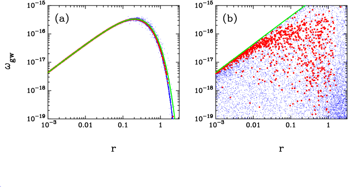
Figure 1: (Colour online) Plots of gravitational wave spectrum $\omega_{\mbox{\scriptsize{gw}}}$ against tensor-to-scalar ratio $r$ for a large number of models evolved with the inflationary flow equations. Square (red) points indicate models satisfying the observational constraints on $n_{s}$ and $dn_{s}/d\ln k$ given by (43). In panel (a), $\omega_{\mbox{\scriptsize{gw}}}$ is calculated using the extrapolation formula (27). The solid line is the first order approximation given by Equation (28). In panel (b), $\omega_{\mbox{\scriptsize{gw}}}$ is calculated using the formula (41). The solid (green) curve in panel (b) shows the bound given by Equation (42), with the parameter $A=7$ .

We ran a program (previously used in gpe ; me ) that generates models of inflation stochastically. The program first selects the initial configuration of a model from uniform distributions within the following ranges:

$$\epsilon_{0} \in [0,0.8]\phantom{t},$$

$$\sigma_{0} \in [-0.5,0.5]\phantom{t},$$

$$\xi_{0} \in [-0.05,0.05]\phantom{t},$$ (36)

$${}^{\ell}\lambda_{H}|_{0} \in [-0.025\times 5^{-\ell+3},0.025\times 5^{-\ell+3}]\phantom{t},\phantom{t}(3\leq\ell\leq 10)$$

$${}^{11}\lambda_{H}|_{0} = 0\phantom{t},$$

where the hierarchy is truncated at $\ell=10$. Each model is evolved forward in time (backward in e-fold) until inflation ends in one of the following ways:

1. By achieving $\epsilon=1$. When this happens, we say for convenience that the ‘slow-roll’ condition has been violated. Observables on CMB scale are then calculated 60 e-folds before the end of inflation. This number of e-fold at which observables are generated is in accordance with the analyses of Refs. leach ; dod .

2. By an abrupt termination, perhaps from intervention of an auxiliary field as in hybrid inflation lr , or, when open strings become tachyonic in brane inflation que ; super1 ; anti . Because these scenarios accommodate a large number of e-folds during inflation, one identifies them with an asymptotic behaviour of a trajectory. In practice, those models inflating for more than $200$ e-folds are grouped under this category. The observables are then calculated along the asymptote.

We produced $10^{6}$ realizations and for each model calculated five key observables, namely $\{r,\phantom{t}n_{s},\phantom{t}n_{T},\phantom{t}dn_{s}/d\ln k,\phantom{t}\omega_{\mbox{\scriptsize{gw}}}\}$. Working with next to leading order expressions in $\epsilon,\eta$, we use the following expression for the primordial tensor power spectra with the assumption that $\epsilon$ and $\eta$ are approximately constant as each mode crosses the Hubble radius sl

$$\mathcal{P}_{T}(k) \simeq {16\over\pi}\left[1-({C+1\over 4})\epsilon\right]^{2}{H^{2}\over m_{\mbox{\scriptsize{Pl}}}^{2}}\bigg{|}_{k=aH},$$ (37)

where $C$ is defined as before. The gravitational wave spectrum depends on Equation (37) evaluated when the direct detection scales cross the Hubble radius. Since modes with frequencies in the direct detection range of around 0.1-1 Hz exit the Hubble radius when $N\simeq 20$, the relation between the Hubble parameters at direct detection and CMB scales is given by

$$H_{\mbox{\scriptsize{direct}}}=H_{\mbox{\scriptsize{CMB}}}\exp\left({-\int^{60}_{20}\epsilon(N)dN}\right)\phantom{t}.$$ (38)

The gravitational wave spectrum is now given in terms of the flow-parameters at scale $k_{0}$ by:

$$\Omega_{\mbox{\scriptsize{gw}}}(k)\simeq{15\over 16H_{0}^{2}k_{\mbox{\scriptsize{eq}}}^{2}\tau_{0}^{4}}\mathcal{P}_{S}(k_{0})r\mathcal{I}(k)\phantom{t},$$ (39)

with $r$ given by Equation (33) and

$$\mathcal{I}(k)=\left[{1-{C+1\over 4}\epsilon(k)\over 1-{C+1\over 4}\epsilon(k_{0})}\right]^{2}\exp\left(-2\int_{20}^{60}\epsilon(N)dN\right)\phantom{t}.$$ (40)

Inserting numerical factors gives:

$$\omega_{\mbox{\scriptsize{gw}}}(k)\simeq 4.36\times 10^{-15}r\mathcal{I}(k)$$ (41)

For comparison between Equation (41) and the extrapolation formula (27), we evaluate the gravitational wave spectrum in our models using both expressions. We adopted a nominal BBO/DECIGO frequency of $0.1$ Hz, consistent with Ref. smith . In any case, the results are insensitive to the choice of frequency as long as the latter exceeds the neutrino damping scale ($\sim 10^{-11}$ Hz).

IV.1 Dependence of $\omega_{\mbox{\scriptsize{gw}}}$ on $r$

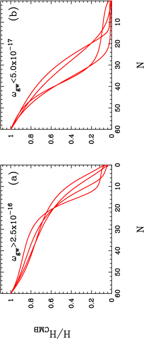
Figure 2: (Colour online) Some trajectories $H(N)$, from CMB scales ($N\simeq 60$) to the end of inflation $(N=0)$, for models evolved using the inflationary flow equations. The models plotted in panel (a) have high gravitational wave amplitudes at direct detection scales ($\omega_{\mbox{\scriptsize{gw}}}>2.5\times 10^{-16}$), whilst those shown in panel (b) have low amplitudes ($\omega_{\mbox{\scriptsize{gw}}}<5\times 10^{-17}$). All of these models satisfy the observational constraints on $n_{s}$ and $dn_{s}/d\ln k$ given by Equation (43), and have high tensor amplitudes in the range $0.15\leq r\leq 0.25$.

Figure 1 summarizes our main results. Most of the models are of the ‘hybrid’ type for which the tensor mode is negligible ($r\approx 0$, $\omega_{\mbox{\scriptsize{gw}}}\approx 0$) and in which the stochastic gravitational wave background is well below the detection threshold of any conceivable experiment. Figure 1a shows the results in the $r-\omega_{\mbox{\scriptsize{gw}}}$ plane when the extrapolation formula (27) is used to compute $\omega_{\mbox{\scriptsize{gw}}}$. Most of the ‘non-trivial’ models (i.e. models with high $\omega_{\mbox{\scriptsize{gw}}}$) lie a few percent below the first order prediction (28) shown by the solid (green) line. All of these non-trivial models achieve $\epsilon=1$ at the end of inflation. Fig. 1b shows the results of using the formula (41) to compute $\omega_{\mbox{\scriptsize{gw}}}$. The distribution of points now spans a large fraction of the $r-\omega_{\mbox{\scriptsize{gw}}}$ plane. The inflationary flow formulation shows that the first order extrapolation formula (27) is too restrictive. Since the shape of the inflationary potential is unknown, it is not possible to extrapolate reliably from CMB scales to the much smaller scales probed by direct detection experiments. Figure 1 shows that it is possible to find inflationary models in which, for instance, the flow variables change rapidly within the last e-folds, thus enhancing $\omega_{\mbox{\scriptsize{gw}}}$ at direct detection scales.

The solid (green) line in Figure 1b shows the expression,

$$\omega_{\mbox{\scriptsize{gw}}}|_{\mbox{\scriptsize{max}}}\simeq 4.36\times 10^{-15}r\left[{1-{C+1\over 64}Ar\over 1-{C+1\over 64}r}\right]^{2}\phantom{t},$$ (42)

where the constant $A\simeq\min\langle\epsilon(k_{0})/\epsilon(k)\rangle$ depends on the distribution (36). In our runs, we find $A\sim 7$. This expression provides an accurate upper bound to $\omega_{\mbox{\scriptsize{gw}}}$. Equation (42) simply expresses the constraint that the Hubble parameter is constant between CMB and direct detection scales, modulated by the term in square brackets which expresses the details of how inflation ends. However, for any value $r\lesssim 1$, the term in square brackets is close to unity and so is insensitive to the parameter $A$ and hence to the distribution (36).

The (red) square points in Figure 1 show the subset of models that satisfy the $2\sigma$ observational constraints seljak ; matteo on $n_{s}$ and $dn_{s}/d\ln k$,

$$0.92\lesssim n_{s}\lesssim 1.06,\quad-1.04\lesssim{dn_{s}\over d\ln k}\lesssim 0.03.$$ (43)

These models roughly follow the locus of the first order extrapolation shown in Figure 1a, but with a large scatter. As a conservative bound we apply Equation (42) with the observational constraint $r<0.36$ seljak , to give

$$\omega_{\mbox{\scriptsize{gw}}}\lesssim 1.6\times 10^{-15}.$$ (44)

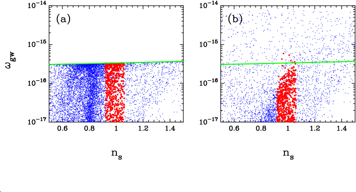
Figure 3: (Colour online) The gravitational wave spectrum $\omega_{\mbox{\scriptsize{gw}}}$ plotted against scalar spectral index $n_{s}$ for a large number of models evolved using the inflationary flow equations. Square (red) points indicate models satisfying the observational constraints on $n_{s}$ and $dn_{s}/d\ln k$ (Equation (43)) and satisfying $r<0.36$. In panel (a), $\omega_{\mbox{\scriptsize{gw}}}$ is calculated using the extrapolation formula (27). The (green) solid curve shows the bound given by Eq. (45). In panel (b), $\omega_{\mbox{\scriptsize{gw}}}$ is calculated using formula (41) and the flow equation integration.

As this paper was nearing completion, a paper by smith2 appeared describing a similar analysis. Our results are broadly compatible, but there appear to be some discrepancies. Comparing our Figure 1b with their Figure 2, we see that the swathe of points satisfying (43) matches roughly the shape of the contoured region in their Figure. However, we find models with low values of $\omega_{\mbox{\scriptsize{gw}}}\lesssim 10^{-18}$ at all values of $r$ whereas they do not. Furthermore, at high values of $r\gtrsim 0.1$, they appear to find models that lie above the bound given by (42). Their results do not seem physically plausible to us .

Examples of some trajectories $H(N)$, from CMB scales to the end of inflation, are shown in Figure 2. All of these models satisfy the observational constraints on $n_{s}$ and $dn_{s}/d\ln k$ of Equation (43) and, in addition, we have imposed the constraint $0.15\leq r\leq 0.25$, i.e. the models have high tensor amplitudes. The models plotted in Figure 2a have high gravitational wave amplitudes at direct detection scales ($\omega_{\mbox{\scriptsize{gw}}}>2.5\times 10^{-16}$). In these cases, the Hubble parameter stays almost constant from $N=60$ to $N=20$ but declines rapidly thereafter. In contrast, the models shown in Figure 2b have low amplitudes $\omega_{\mbox{\scriptsize{gw}}}<5\times 10^{-17}$. In these cases, $H(N)$ declines more rapidly between $N=60$ and $N=20$. These sample trajectories show that models with sharp features in $H(N)$ (and hence also in $V(\phi)$) within the last $20$ e-folds of inflation will be the first to be ruled out by BBO/DECIGO-type detectors.

IV.2 Dependence of $\omega_{\mbox{\scriptsize{gw}}}$ on scalar tilt $n_{s}$

Figure 3 shows the models plotted in the $n_{s}-\omega_{\mbox{\scriptsize{gw}}}$ plane. The extrapolation method (Fig. 3a) places most of the ‘non-trivial’ models within a vertical band centered around $n_{s}\sim 0.8$. The band is sharply capped by the solid (green) curve given by differentiating Eq.(27):

$$\omega_{\mbox{\scriptsize{gw}}}|_{\mbox{\scriptsize{max}}}=4.24\times 10^{-17}\left[{17.235-1.303n_{s}\over 2.565-0.541n_{s}}\right],$$ (45)

Fig.3b shows the distribution when the flow formulation (41) is used to calculate $\omega_{\mbox{\scriptsize{gw}}}$. The region beyond the envelope (45) is now populated by many models, some of which produce $\omega_{\mbox{\scriptsize{gw}}}$ in excess of $10^{-14}$. However, all of the models with such high values of $\omega_{\mbox{\scriptsize{gw}}}$ are inconsistent with the observational constraints on $n_{s}$ and $dn_{s}/d\ln k$. The (red) squares in Figure 3 indicate models that satisfy the $2\sigma$ observational constraints of Equation (43), and, in addition, have $r<0.36$. The vast majority of these models lie below the line defined by Equation (45). However, it is possible, though rare, for models satisfying the observational constraints (43) to exceed $\omega_{\mbox{\scriptsize{gw}}}>3\times 10^{-16}$, as given by Equation (45). Evidently, one can see from Figure 1b that no model satisfying the observational constraints can exceed our conservative bound (44).

V Prospects for direct detection

The results of the preceding Section show that simple single-field inflation models must satisfy the conservative constraint of Equation (44) at direct detection scales. Furthermore, unless the inflationary parameters are specially tuned, most single-field inflation models will produce $\omega_{\mbox{\scriptsize{gw}}}\lesssim 3\times 10^{-16}$. Thus, at the BBO/DECIGO sensitivities of $\sim 10^{-15}-10^{17}$ (see Table 1), a direct detection of a stochastic background of gravitational waves would be expected only if the inflationary potential contains a feature at $N\sim 20$, as shown in the trajectories plotted in Figure 3. This is true even if the tensor-to-scalar ratio is high at CMB scales. This is the main conclusion of this paper.

Although this may seem a somewhat pessimistic conclusion for direct detection experiments, it is worth mentioning a range of other cosmological sources (summarized in Table II) that could produce a stochastic background of gravitational waves at direct detection scales.

(i) Pathological potential: A sudden decrease in energy scale of the inflationary universe could be attributed to a first order phase transition brought about by the spontaneous symmetry breaking of a field coupled to the inflaton. As a result, the potential $V(\phi)$ also acquires a sharp feature in the form of steps double ; doubles ; park ; adams , kinks starobinsky ; lesga ; lesgb or combination of these at various scales ars . In particular, the primordial gravitational wave amplitude in the so-called ‘broken-scale invariance’ models has been considered in Refs. smith ; polarski , which found roughly an order of magnitude increase above that given by Equation (28). Clearly, a first order phase transition has a negligible enhancement effect on modes at direct detection scales unless the transition occurs at late stages (within the last $\sim$20 e-folds) of inflation. On the other hand, if scale invariance is broken at around the CMB/LSS scales, as suggested by Mukherjee ; einasto ; gaztanaga , then the gravitational wave amplitude may be enhanced at scales probed by the future CMB polarization experiments.

(ii) Bubble nucleation: A phase transition may also be accompanied by a rapid nucleation of vacuum bubbles highest ; extended1 ; extended2 , which upon collision during inflation produce a large gravitational wave background with $\omega_{\mbox{\scriptsize{gw}}}$ of order $\sim 10^{-7}$ around the direct detection frequencies. However, bubble collision at a much lower energy, e.g. the electroweak scale, produces virtually negligible gravitational waves with $\omega_{\mbox{\scriptsize{gw}}}$ of order $10^{-23}$ turbo . In supersymmetric extentions of the standard model, this value may be larger by several orders of magnitude mssm and perhaps as large as $\sim 10^{-11}$ for some parameter choices in next-to-minimal models.

(iii) Turbulence: A large injection of energy into the cosmological plasma following bubble collision could also set up a Kolmogorov spectrum of turbulence. Calculations in Refs. turbo ; turbo2 estimate the gravitational wave background from turbulence to be comparable to that from bubble nucleation. If the turbulence is sourced also by a helical field (e.g. primordial magnetic fields), a secondary contribution of $\omega_{\mbox{\scriptsize{gw}}}\sim 10^{-11}$ is predicted at direct detection scales ratra . Relation between $\omega_{\mbox{\scriptsize{gw}}}$ and the strength of primordial magnetic fields is further discussed in durrer1 ; durrer2

(iv) Cosmic strings: A stochastic network of strings sv ; kibble produces a gravitational wave spectrum with a long plateau extending from $f\sim 10^{-10}$ Hz across direct detection scales u1 ; u2 . Although CMB observations show that strings cannot be solely responsible for structure formation wyman , they can arise in certain models of hybrid and brane inflation as a sub-dominant contribution to the fluctuations super1 ; super2 ; Firouzjahi . Recently Refs. cusp1 ; cusp2 have calculated the gravitational wave spectrum from bursts associated with cusps and kinks in loops of cosmic (super)strings as a function of the theoretically uncertain intercommutation probability. They conclude that the gravitational wave bursts from strings with tensions as low as $G\mu\sim 10^{-14}$ could result in $\omega_{\mbox{\scriptsize{gw}}}$ as large as $\sim 10^{-11}$. This is potentially detectable by LISA and may even be observable by LIGO if $G\mu\gtrsim 10^{-10}$ and the intercommutation probablity small.

While inflation may be accompanied by all of the phenomena mentioned above, some alternatives to slow-roll inflation have altogether different predictions regarding the production of primordial gravitational waves at direct detection scales.

(v) Pre-Big Bang and cyclic models: In Pre-Big Bang scenarios sdual ; vene , a dilaton-driven phase with $\dot{H}>0$ gives rise to a gravitational wave amplitude which increases with frequency ($\sim f^{3}$) for all modes exiting the Hubble radius during the Pre-Big Bang era. The primordial tensor spectrum in this case is strongly blue with $n_{T}=3$. The gravitational wave spectrum could peak at direct detection scales with amplitude $\omega_{\mbox{\scriptsize{gw}}}$ as high as $10^{-6}$, within reach of advanced terrestrial detectors pbb1 ; pbb2 ; pbb3 . When combined with CMB polarization experiments, a strongly blue tensor spectrum can be easily ruled out. Nevertheless, the prediction of such a large gravitational wave amplitude at direct detection scales is sensitive to physics during the ‘bounce’ around $t=0$, which remains poorly understood review . In contrast, the cyclic model cyclic ; cyclicbig predicts a blue tensor spectrum ($n_{T}=2$) but with negligible gravitational wave amplitude at direct detection scales cygw .

(vi) Braneworlds: Inflation has been implemented in 5-dimensional phenomenological braneworld models rs1 ; rs2 ; trap . Gravitational waves at direct detection scales cross the Hubble radius at high energies ($H\ell\gg 1$, where $\ell$ is the bulk curvature), hence $\omega_{\mbox{\scriptsize{gw}}}$ is directly affected by extra-dimensional physics. An enhancement effect in $\omega_{\mbox{\scriptsize{gw}}}$ arises through the modification of the Friedmann equation, whereas a damping effect occurs via the mixing of massive Kaluza-Klein modes with the massless graviton hira1 ; mix ; ichiki . At direct detection scales, it is conceivable that these two effects cancel hira2 ; cancel .

ttttPhenomena	Key parameters	$\omega_{\mbox{\scriptsize{gw}}}$(1 mHz - 1 Hz)	References
1. Slow-roll inflation	Inflationary energy scale.	$\lesssim 10^{-15}$	Eq. (44)
2. Pathological potential		$\lesssim 10^{-15}$t	smith ; polarski
3. Bubble nucleation		$\lesssim 10^{-7}$ $10^{-11}-10^{-16}$ $10^{-23}$	highest ; extended1 ; extended2 mssm turbo
4. Turbulence		$\lesssim 10^{-7}$ $10^{-12}$	turbo ; turbo2 ratra
5. Cosmic strings		$10^{-9}-10^{-11}$	cusp2
6. Pre-Big Bang / Cyclic tttmodels		$\lesssim 10^{-6}$ $10^{-35}$	pbb1 ; pbb2 ; pbb3 cygw
7. Braneworlds		$\lesssim 10^{-16}$	ichiki ; cancel

Table 2: Summary of some possible cosmological sources of primordial gravitational wave background in the frequency range of future direct detection experiments ($f\simeq$ 1 mHz - 1 Hz). Inflation may be accompanied by some (or all) of phenomena 2-5, while phenomena 6 and 7 are alternatives to the inflationary scenario.

Finally it is worth noting that we have ignored astrophysical sources, most notably from inspiralling binary systems of white dwarfs, neutron stars or black holes which could produce a significant background at frequencies of 1 mHz to $1$ Hz. These sources must be subtracted to high accuracy astro ; cooray ; harms to achieve sensitivities of $\omega_{\mbox{\scriptsize{gw}}}\ll 10^{-15}$ necessary to test inflation, and may ultimately limit direct detection experiments. The sensitivities of the post-LISA experiments quoted in Table I depend on the usable frequency range and are significantly lower if frequencies $\lesssim 0.2$ Hz are contaminated by a high background from unresolved white dwarfs.

VI Conclusions

The generation of tensor modes is a key prediction of inflationary models and has yet to be confirmed by experiment. A large experimental effort is underway to detect a tensor mode signature in the polarization of the CMB. On a longer time-scale, a number of direct detection experiments have been proposed to detect a stochastic background of gravitational waves at frequencies in the range 1 mHz - 1 Hz. However, since the spatial scales probed by direct experiments are some $15$ orders of magnitude smaller than the scales probed by the CMB, extrapolating between these scales is highly model dependent turnerlett ; smith .

In this paper, we have used the inflationary flow equations to assess the accuracy of extrapolating between CMB and direct detection scales for single-field inflationary models. Our main results are shown in Figures 1 and 3. For models that satisfy the observational constraints on $n_{s}$ and $dn_{s}/d\ln k$, we find a conservative upper bound of $\omega_{\mbox{\scriptsize{gw}}}\lesssim 1.6\times 10^{-15}$. However, as shown in Figure 3b most of our models have much lower values of $\omega_{\mbox{\scriptsize{gw}}}$, and only a small minority have $\omega_{\mbox{\scriptsize{gw}}}\gtrsim 3\times 10^{-16}$. A direct detection experiment with a sensitivity of $\omega_{\mbox{\scriptsize{gw}}}\sim 10^{-16}$ is therefore limited to testing a range of single field inflationary models in which the Hubble parameter is roughly constant between CMB scales ($N\approx 60$) and direct detection scales ($N\approx 20$), followed by an abrupt decline thereafter. Examples of such trajectories are shown in Figure 2a.

We have also identified a number of cosmological sources of stochastic gravitational wave background accessible to direct detection experiments (Table II). In some cases, the predicted amplitudes are far in excess of those generated during inflation. A high value of $\omega_{\mbox{\scriptsize{gw}}}$ from, say, cosmic strings produced at the end of brane inflation might easily overwhelm the contribution from tensor modes generated during inflation. In more general scenarios, therefore, it may be difficult for direct detection experiments to constrain the inflationary phase even if experiments can achieve ‘Ultimate DECIGO’ sensitivities of $\omega_{\mbox{\scriptsize{gw}}}\sim 10^{-20}$.

Acknowledgments: We thank Antony Lewis for useful discussions. SC acknowledges the support of a Dorothy Hodgkin scholarship from PPARC. This work has been supported by PPARC.

References

- (1) Weber J., Phys. Rev. Lett. 22, 1320 (1969).
- (2) Turner M.S., Phys. Rev. D 55, R435 (1997).
- (3) Smith T.L., Kamionkowski M. and Cooray A., Phys. Rev. D 73, 023504 (2006).
- (4) http://www.ligo.caltech.edu/advLIGO
- (5) Pizzella G., Di Virgilio A., Bender P. and Fucito F., Gravitational Waves, Series in High Energy Physics, Cosmology and Gravitation (eds. Ciufolini I., Gorini V., Moschella U. and Fré P.) , Institute of Physics Publishing, pp. 115 (2001)
- (6) Corbin V. and Cornish N.J., arXiv:gr-qc/0512039.
- (7) Seto N., Kawamura S. and Nakamura T., Phys. Rev. Lett. 87, 221103 (2001).
- (8) Kudoh H., Taruya A., Hiramatsu T. and Himemoto Y., gr-qc/0511145.
- (9) Lidsey J.E., Liddle A.R., Kolb E.W., Copeland E.J., Barreiro T. and Abney M., Rev. Mod. Phys. 69, 373 (1997).
- (10) Stewart E.D. and Lyth D.H., Phys. Lett. B 302, 171 (1993).
- (11) Efstathiou G. and Mack K.J., JCAP 0505 008 (2005).
- (12) Peiris H.V., et al. Ap.J. Suppl., 148, 213 (2003).
- (13) Chongchitnan S. and Efstathiou G., Phys. Rev. D 72, 083520 (2005).
- (14) Liddle A.R. and Lyth D.H., ‘Cosmological Inflation and Large-Scale Structure’, Cambridge University Press (2000).
- (15) Turner M.S., White M. and Lidsey J.E., Phys. Rev. D 48, 4613 (1993).
- (16) Turner M.S. and White M., Phys. Rev. D 53,6822 (1996).
- (17) Maggiore M., Phys.Rept. 331, 283 (2000).
- (18) Buonanno A., arXiv:gr-qc/0303085.
- (19) Dodelson S., ‘Modern Cosmology’, Academic Press (2003).
- (20) Boyle L. and Steinhardt P.J., arXiv:astro-ph/0512014
- (21) Isaacson R.A., Phys. Rev. 166 1263-1280 (1968).
- (22) Seljak U. et. al., Phys. Rev. D 71, 103515 (2005).
- (23) Weinberg S., Phys. Rev. D 69, 023503 (2003).
- (24) Bond J.R., Cosmology and Large Scale Structure, Les Houches Session LX, August 1993, eds. Schaeffer R., Silk J., Spiro M. and Zinn-Justin J., Elsevier, Amsterdam (1996).
- (25) Hoffman M.B. and Turner M.S., Phys. Rev. D 64, 023506 (2001).
- (26) Kinney W.H., Phys. Rev. D 66, 083508 (2002).
- (27) Ramirez E. and Liddle A.R., Phys. Rev. D 71, 123510 (2005).
- (28) Liddle A.R., Phys. Rev. D68, 103504 (2003).
- (29) Easther R. and Kinney W.H., Phys. Rev. D 67, 043511 (2003).
- (30) Liddle A.R., Parsons P. and Barrow J.D., Phys. Rev. D 50, 7222 (1994).
- (31) Seto N., Phys. Rev. D 73, 063001 (2006).
- (32) Song Y.-S. and Knox L., Phys.Rev. D68, 043518 (2003).
- (33) Cortês M. and Liddle A.R., arXiv:astro-ph/0603016
- (34) Liddle A.R. and Leach S.M., Phys. Rev. D 68, 103503 (2003).
- (35) Dodelson S. and Hui L., Phys. Rev. Lett. 91, 131301 (2003).
- (36) Lyth D.H. and Riotto A., Phys.Rept. 314, 1 (1999).
- (37) Quevedo F., Class.Quant.Grav. 19, 5721 (2002).
- (38) Sarangi S. and Tye S.-H.H., Phys.Lett. B 536, 185 (2002).
- (39) Burgess C.P. et al. , JHEP 07, 047 (2001).
- (40) Viel M., Weller J. and Haehnelt M., MNRAS 355, L23 (2004).
- (41) Smith T.L., Peiris H.V. and Cooray A., arXiv:astro-ph/0602137
- (42) Silk J. and Turner M.S., Phys. Rev. D 35, 419 (1987).
- (43) Copeland E.J., Liddle A.R., Lyth D.H., Stewart E.D. and Wands D., Phys. Rev. D 49, 6410 (1994).
- (44) Parkinson D., Tsujikawa S., Bassett B.A. and Amendola L., Phys. Rev. D 71, 063524 (2005).
- (45) Adams J., Cresswell B. and Easther R., Phys. Rev. D 64, 123514 (2001).
- (46) Starobinsky A.A., JETP Lett. 55, 489 (1992).
- (47) Lesgourgues J., Polarski D. and Starobinsky A.A., MNRAS 297, 769 (1998).
- (48) Lesgourgues J., Polarski D. and Starobinsky A.A., MNRAS 308, 281 (1999).
- (49) Adams J., Ross G. and Sarkar S., Nucl. Phys. B 503, 405 (1997).
- (50) Polarski D., Phys. Lett. B 458, 13 (1999).
- (51) Mukherjee P. and Wang Y., Astrophys. J. 599, 1 (2003).
- (52) Einasto J. et al. , Astrophys. J. 519, 469 (1999).
- (53) Gaztañaga E. and Baugh C.M., MNRAS 294, 229 (1998).
- (54) Baccigalupi C., Amendola L., Fortini P. and Occhionero F., Phys. Rev. D 56, 4610 (1997).
- (55) La D. and Steinhardt P.J., Phys. Rev. Lett. 62, 376 (1989).
- (56) Turner M.S. and Wilczek F., Phys. Rev. Lett. 65, 3080 (1990).
- (57) Kamionkowski M., Kosowsky A. and Turner M.S., Phys. Rev. D 49, 2837 (1994).
- (58) Apreda R., Maggiore M., Nicolis A. and Riotto A., Class. Quant. Grav. 18, L155 (2001).
- (59) Kosowsky A., Mack A. and Kahniashvili T., Phys. Rev. D 66, 024030 (2002).
- (60) Kahniashvili T., Gogoberidze G. and Ratra B., Phys. Rev. Lett. 95 151301 (2005).
- (61) Caprini C. and Durrer R., Phys.Rev. D 65, 023517 (2002).
- (62) Caprini C. and Durrer R., Phys.Rev. D 72, 088301 (2005).
- (63) Vilenkin A. and Shellard E.P.S., ‘Cosmic Strings and Other Topological Defects’, Cambridge University Press (1994).
- (64) Hindmarsh M.B. and Kibble T.W.B. , Rept. Prog. Phys. 58, 477 (1995).
- (65) Caldwell R.R. and Allen B., Phys. Rev. D 45, 3447 (1992).
- (66) Caldwell R.R., Battye R.A. and Shellard E.P.S., Phys. Rev. D 54, 7146 (1996).
- (67) Wyman M., Pogosian L. and Wasserman I., Phys. Rev. D 72, 023513 (2005).
- (68) Jones N., Stoica H. and Tye S.-H.H, JHEP 0207, 051 (2002).
- (69) Firouzjahi H. and Tye S.-H.H, JCAP 0503, 009 (2005).
- (70) Damour T. and Vilenkin A., Phys. Rev. D 64, 064008 (2001).
- (71) Damour T. and Vilenkin A., Phys. Rev. D 71, 063510 (2005).
- (72) Veneziano G., Phys. Lett. B 265, 287 (1991).
- (73) Veneziano G., arXiv:hep-th/9802057.
- (74) Allen B. and Brustein R., Phys. Rev. D 55, 3260 (1997).
- (75) Buonanno A., Maggiore M. and Ungarelli C., Phys. Rev. D 55, 3330 (1997).
- (76) Gasperini M., Chapter 16 in Ref. lisa .
- (77) Veneziano G. and Gasperini M., Phys. Rept. 373, 1 (2003).
- (78) Steinhardt P.J. and Turok N., Phys. Rev. D 65, 126003 (2002).
- (79) Khoury J., Ovrut B.A., Steinhardt P.J. and Turok N., Phys. Rev. D 64, 123522 (2001).
- (80) Boyle L.A., Steinhardt P.J. and Turok N., Phys. Rev. D 69, 127302 (2004).
- (81) Randall L. and Sundrum R., Phys. Rev. Lett. 83, 3370 (1999).
- (82) Randall L. and Sundrum R., Phys. Rev. Lett. 83, 4690 (1999).
- (83) Shiromizu T., Maeda K. and Sasaki M., Phys. Rev. D 62, 024012 (2000).
- (84) Hiramatsu T., Koyama K. and Taruya A., Phys.Lett. B578, 269 (2004).
- (85) Easther R., Langlois D., Maartens R. and Wands D., JCAP 0310, 014 (2003).
- (86) Ichiki K. and Nakamura K., arXiv:astro-ph/0406606.
- (87) Hiramatsu T., Koyama K. and Taruya A., Phys.Lett.B609, 133 (2005).
- (88) Kobayashi T. and Tanaka T., Phys. Rev. D 73, 044005 (2006).
- (89) Cutler C. and Thorne K.S., arXiv: gr-qc/0204090.
- (90) Cooray A., Mod. Phys. Lett. A, 20, 2503 (2005).
- (91) Cutler C. and Harms J., Phys. Rev. D 73, 042001 (2006).