GalaxyCount: a java calculator of galaxy counts and variances in multiband wide-field surveys to 28 AB mag

Abstract

We provide a consistent framework for estimating galaxy counts and variances in wide-field images for a range of photometric bands. The variances include both Poissonian noise and variations due to large scale structure. We demonstrate that our statistical theory is consistent with the counts in the deepest multiband surveys available. The statistical estimates depend on several observational parameters (e.g. seeing, signal to noise ratio), and include a sophisticated treatment of detection completeness. The java calculator is freely available¹ and offers the user the option to adopt our consistent framework or a different scheme. We also provide a summary table of statistical measures in the different bands for a range of different fields of view.

Reliable estimation of the background counts has profound consequences in many areas of observational astronomy. We provide two such examples. One is from a recent study of the Sculptor galaxy NGC 300 where stellar photometry has been used to demonstrate that the outer disc extends to 10 effective radii, far beyond what was thought possible for a normal low-luminosity spiral. We confirm this finding by a reanalysis of the background counts. Secondly, we determine the luminosity function of the galaxy cluster Abell 2734, both through spectroscopically determined cluster membership, and through statistical subtraction of the background galaxies using the calculator and offset fields. We demonstrate very good agreement, suggesting that expensive spectroscopic follow-up, or off-source observations, may often be bypassed via determination of the galaxy background with GalaxyCount.

1 Introduction

With the advent of wide-field imagers on high-quality observing sites, there are increasing numbers of very deep, wide-angle studies (e.g. nearby galaxies) that are subject to an unknown contribution of background galaxy counts. Even when the same field has been observed in several photometric bands, it can be very difficult to remove correctly the background galaxy counts at a deep magnitude limit.

The issue of background contamination is likely to persist for many years. Even with the fine resolution ($\approx 0.1"$) of the Hubble Space Telescope (HST) the highest redshift sources are still largely unresolved (Ouchi et al. 2005). Therefore star/galaxy discrimination of such objects awaits the development of multi-conjugate adaptive optics (MCAO) capable of spatial resolution on the order of tens of milli-arcseconds. However, higher resolution observations will result in a smaller field of view (FOV), since the focal plane of any instrument can only be populated with a limited number of CCDs. A “wide-field imager” in an era of MCAO is unlikely to exceed a few arcminutes (Bland-Hawthorn 2006). A smaller FOV results in poorer statistical subtraction of background galaxies, due to larger relative uncertainty on the number counts.

We provide a java calculator for estimating these variations in several photometric bands over a wide magnitude range. Our analytic approach is supported by the deepest surveys to date. Our modelled magnitude limits are ($U,B,R,I,K$) $\approx$ (27, 29, 28, 28, 23) mag.

We first describe our model in Section 2 and then present the results of the model with comparison to the Subaru Deep Field (SDF) in Section 3. Section 4 describes worked examples of two practical applications of the model. First to a study of star-counts in NGC 300 by Bland-Hawthorn et al. (2005), and secondly to the determination of galaxy cluster luminosity functions. Finally we discuss the results and present our conclusions in Section 5.

We have assumed a cosmology of $H_{0}=70$ km s^-1 Mpc^-1, $\Omega_{{\rm M}}=0.3$ and $\Omega_{\Lambda}=0.7$ throughout, although the results are not very sensitive to the exact choice of cosmology.

2 Predicting counts and variances

The variance of galaxy number counts in a randomly placed cell of solid angle $\Omega$ is given by,

$$\sigma^{2}=n\Omega+n^{2}\int{\rm d}\Omega_{1}{\rm d}\Omega_{2}\omega(\theta_{12}),$$ (1)

where $n$ is the number density of galaxies, and ${\rm d}\Omega_{1}$ and ${\rm d}\Omega_{2}$ are elements of the solid angle $\Omega$ separated by an angle $\theta_{12}$ (Peebles 1980). The angular correlation function $\omega$ can be parametrized as,

$$\omega(\theta)=A\theta^{-\delta}.$$ (2)

Following Peebles (1975) we change variables to rewrite equation 1 as,

$$\sigma^{2}=n\Omega+(n\Omega)^{2}A\theta_{\rm C}^{-\delta}\int\frac{{\rm d}^{2}x_{1}{\rm d}^{2}x_{2}}{|{\bf x_{1}}-{\bf x_{2}}|^{\delta}},$$ (3)

where the integral on the right hand side is an integral over the cell scaled to unit area, and the scale factor of the cell $\theta_{\rm C}$ has been taken out of the integral. For a square cell of side $\theta_{\rm C}$ the integral equates to 2.24 (Peebles 1975), for a circular cell the integral equates to $\approx 1.53$ with $\theta_{\rm C}$ equal to the diameter of the cell (found by numerical integration). GalaxyCount also allows oblong and elliptic window functions, which are integrated numerically within the code.

Thus in order to calculate the variance for any general observation of a given area and depth, it is necessary to know how the number density and the correlation function amplitude change as a function of magnitude in the appropriate waveband. These will now be considered in turn.

2.1 Number density

A large number of published galaxy number count surveys exist in many different wavebands. These have been compiled for the $UBRIK$ filters to yield the differential number density over a wide range of magnitudes ($18.375\leq U\leq 27.45$, $10.45\leq B\leq 29.35$, $14.42\leq R\leq 28.37$, $12.25\leq I\leq 28.25$, $9.37\leq K\leq 23.48$). The list of sources used in this work is given in appendix A.1.

Thus the number density may be computed through integration over the required magnitude range. In practice this is achieved by averaging all the data in bins of width 1 mag, and fitting a cubic spline through the resulting averages. The spline is then integrated numerically.

2.1.1 Completeness

A very important caveat with the above method is that the published number density surveys have all been corrected for incompleteness at their faintest magnitudes in order to estimate the true number counts of galaxies (which is necessary to accurately derive cosmological models, etc.). However, if the variance of galaxy counts is required to estimate how accurately the foreground/ background galaxies can be removed from an observation the above method will yield incorrect results. The completeness of the observations must be accounted for. Fewer counts will be made at the faintest magnitudes, and hence the contribution to the variance will decrease. Because the number density is very high at faint magnitudes, the contribution from the faintest galaxies dominates the calculation, therefore it is imperative to accurately account for any incompleteness.

We define completeness as the number of galaxies detected divided by the true number of galaxies. In practice the completeness is usually estimated by artificially generating galaxies of various magnitude and adding these to the images. The completeness can then be estimated by running the source detection software and counting the number of artificial objects which have been recovered. Thus the completeness will depend on the source detection algorithm and thresholds. In particular the completeness function will change with the significance of the detection threshold, e.g. a 5$\sigma$ detection threshold (i.e. the flux of detected sources is $\geq 5\sigma$ above the background) will have brighter completeness limits than a 3$\sigma$ detection threshold.

The detection threshold also determines the effect of spurious detections, such that a higher threshold will have fewer spurious detections. GalaxyCount does not account for spurious detections, which would be few for typical detection thresholds of $\geq 3\sigma$. This should be borne in my mind by the user if it is expected that there are many spurious detections in their data.

The completeness for any observation depends on the telescope aperture, the combined throughput of the telescope, instrument and atmosphere, the exposure time, the seeing ($\Gamma$) and the signal to noise ratio (SNR) of the detections, providing that the seeing is well sampled. Thus if the completeness function is known for any observation it may easily be scaled for any other observation, on the assumption that the shape of the curve does not change. Furthermore the completeness function can be modelled using a sigmoid function of the form,

$$f=\frac{1}{1+e^{a(x-b)}},$$ (4)

where $f=N_{{\rm measured}}/N_{{\rm true}}$ is the completeness, $b$ is the magnitude at which $f=0.5$, and $a$ (which has units of magnitudes^-1) determines the sharpness of the step.

It is essential to use a sigmoid completeness function that correctly matches the observations in question, i.e. $a$ and $b$ must be correctly chosen. This is very important because the galaxy number counts rise rapidly at faint magnitudes, and a change in the completeness function can have a large effect on the mean number counts and associated error. In Figure 1 we have compiled various completeness functions from the literature and our own data to show the spread in sigmoid slope which results from different object detection methods. Object detection optimised for galaxies generally yield a flatter slope than those optimised for point source detection. Similarly adaptive optics corrected images seem to result in a steeper slope than natural seeing images. These trends are easily understood as extended sources of fixed magnitude will have a greater range of surface brightness than point sources of fixed magnitude. Thus there is a larger spread in the sigmoid transition for extended sources as some faint magnitude may have a high central surface brightness and thus be detected, whereas some bright magnitude sources may have an overall low surface brightness and thus be missed. Only sigmoid functions derived from extended source detections should be used with GalaxyCount because of this difference. GalaxyCount uses a default slope of $a=3.0$, which is typical for galaxy detections, however we stress that to obtain accurate results the completeness function for the users own data should be computed. This illustrated in Figure 2, which shows the effect of varying the slope of the sigmoid function for B band observations with $18\leq B\leq 27$ mag and a fixed 50 per cent completeness of B=27 mag.

Figure 1: Completeness functions compiled from the literature and our own data, all translated to have 50 per cent completeness at zero magnitude. The points show the data from: the Subaru Deep Field B band galaxy counts (open circles, Kashikawa et al. 2004); the author’s own GMOS g band observations of a redshift 0.7 cluster of galaxies (open squares); the author’s own IRIS2 K band observations of the same field (open triangles); ISAAC 1.19$\mu m$ narrow band filter data of the Chandra Deep Field South (closed circles, Cuby et al. 2007); NACO AO corrected observations (closed squares, Cresci et al. 2006); the author’s own GMOS r band imaging for point sources (closed triangles, Bland-Hawthorn et al. 2005); NACO AO corrected observations for point sources (stars, Cresci et al. 2006). The lines show the best fitting sigmoid functions and range from $a=1.4$ for the SDF observations to $a=6.0$ for the NACO AO corrected point sources.

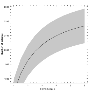
Figure 2: The effect of the sigmoid slope on the resulting number counts and standard deviation for $18\leq B\leq 27$ in a $5\times 5^{\prime}$ area, with a fixed 50 per cent completeness of 27 mag. The solid line shows the number counts and the shaded area the 1$\sigma$ uncertainty on those counts.

GalaxyCount uses a default sigmoid with $a=3.0$ which may be used to provide an estimate the expected completeness of any observation by scaling $b$ appropriately. The $b$ values were measured from the SDF $B$, $R$ and $I$ completeness functions in Kashikawa et al. (2004), and converted to Vega magnitudes using the transformations given in section 2.4 ($U$ was derived from the B band completeness function), and the SDF $K$ band completeness function was measured from Maihara et al. (2001). In order to allow scaling from the SDF observations we have taken throughputs for Suprime-Cam $BRI$ (actually $i^{\prime}$) from Miyazaki et al. (2002) (convolved with Mauna Kea atmospheric transmission from Hook et al. 2004), and for CISCO $K$ from Motohara et al. (2002), we have assumed the GMOS throughput for $U$. We also offer the Gemini GMOS throughputs from Hook et al. (2004) as a default option in the calculator (we assume that the $u^{\prime}g^{\prime}r^{\prime}i^{\prime}$ throughputs are appropriate for $UBRI$, and we assume the CISCO $K$ band throughput is appropriate for Gemini NIR imagers).

Provision is made for the user to override any of our assumptions when using the calculator. Observing conditions, telescope aperture and instrument throughput may all be freely specified, or a particular sigmoid completeness function may be input. To give an impression of the importance of correctly specifying the appropriate observing conditions etc.  Figure 3 shows the effect of varying the throughput on the resulting $18\leq B\leq 27$ mag number counts and standard deviation in a $5\times 5^{\prime}$ area, for a 595 minute exposure, with SNR=3, $\Gamma\approx 1"$, on an 8m aperture telescope. Clearly it is important to use the correct input for the particular observations of concern.

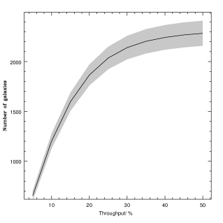
Figure 3: The effect of the throughput on the resulting number counts and standard deviation for $18\leq B\leq 27$ in a $5\times 5^{\prime}$ area, for a 595 minute exposure, with SNR=3, $\Gamma\approx 1"$, on an 8m aperture telescope. The solid line shows the number counts and the shaded area the 1$\sigma$ uncertainty on those counts.

The difference in standard deviation resulting from incomplete and corrected observations is shown in Figure 4, for a $5^{\prime}\times 5^{\prime}$ FOV for a series of different exposure times and faint magnitude limits, with the other observing conditions the same as for the SDF.

Figure 4: The expected number, standard deviation, and standard deviation divided by square root of the number (i.e. the non-Poissonian component of the standard deviation) of galaxies in surveys of different magnitude limits, with a $5^{\prime}\times 5^{\prime}$ FOV. The thick black line is for the total number of galaxies, the dotted and dashed lines include estimates for the incompleteness of the observations for exposure times of 595, 300 and 10 minutes, with SNR=3, $\Gamma\approx 1"$, with an 8m aperture telescope with 36% throughput and deviate from the thick black line in that order.

Of course the number of galaxies in the field may already be known, and therefore GalaxyCount includes provision for the user to enter his or her own value, as well as providing estimates from including and excluding incompleteness. The standard deviation $\sigma_{2}$ associated with a measured number of galaxies, $N_{2}$, counted in a particular magnitude range and area, may be scaled from the predicted number and standard deviation, $N_{1}$ and $\sigma_{1}$, assuming the amplitude of the angular correlation function is the same in both observations, through the equation,

$$\sigma_{2}=\sqrt{f^{2}\sigma_{1}^{2}+N_{1}f(1-f)},$$ (5)

which may be combined with equation 4, to scale the results presented in Table 1 for different values of completeness.

2.2 Stellar contamination

The severity of stellar contamination will depend on the direction of the observations. Stars are not expected to contribute significantly to the number counts for observations away from the Galactic plane (Robin et al. 2003). Bright stars may be easily removed from the catalogues via visual inspection, radial profile fitting or automatic discrimination (e.g. Bertin & Arnouts 1996). At fainter magnitudes the stellar contamination will not be significant. Figure 5 compares the expected contribution of star counts at a Galactic latitude of $b=90$ degrees and longitudes $l=0,90,270$ degrees to the $K$ band galaxy counts compiled from the literature (see appendix A.1. If stellar contamination is expected to be a problem then it can be accounted for using synthetic models such as those of Robin et al. (2003).

Figure 5: The modelled star counts from Robin et al. (2003) compared to galaxy counts compiled from the literature shown by the points.

2.3 Amplitude of the angular correlation function

The amplitude of the angular correlation function decreases at fainter magnitudes, since the average redshift of the sample is larger and hence the volume being surveyed is larger, and thus the distribution of galaxies is approaching homogeneity.

The functional dependence of $A$ on magnitude has been reported to be monotonically declining (e.g. McCracken et al. 2001; Wilson 2003; Coil et al. 2004) or to flatten off at the faintest magnitudes (e.g. Brainerd & Smail 1998; Postman et al. 1998). Both possibilities have been modelled in GalaxyCount, and the user may choose between them. The first case was simply modelled by a least squares fit to log$A$ vs. magnitude for data compiled from the literature. However, to allow the models to be extrapolated to very faint magnitudes the second case has also been modelled, which allows for a flattening of $A$ at faint magnitudes. The sources for the measurements of the angular correlation function used in this paper are listed in appendix A.2.

The amplitude of the angular correlation function has been modelled using theoretical arguments describing the evolution of clustering, in particular Efstathiou et al. (1991) and Peebles (1980). The method takes a parametrized evolution of the two-point spatial correlation function and converts it to the expected dependence of $A$ on magnitude. The two-point spatial correlation function is usually parametrized as,

$$\xi(r)=\left(\frac{r_{0}}{r}\right)^{\gamma}.$$ (6)

The scaling of $\xi(r)$ with redshift, $z$, may be parametrized as (Groth & Peebles 1977),

$$\xi(r,z)=h(z)\left(\frac{r_{0}}{r}\right)^{\gamma},$$ (7)

where

$$h(z)=(1+z)^{-(3+\epsilon)},$$ (8)

where $r$ is the proper distance and $\epsilon$ describes the evolution of the clustering, with

$$\epsilon=\left\{\begin{array}[]{ll}0&\mbox{-- clustering fixed in proper co-ordinates}\\ -1.2&\mbox{-- clustering fixed in comoving co-ordinates}\\ 0.8&\mbox{-- prediction of linear theory.}\end{array}\right.$$ (9)

In all cases with $\epsilon>-1.2$ the comoving galaxy correlation length decreases monotonically with $z$. GalaxyCount uses $\epsilon=-1.2,0,0.8,3$ as selected by the user; $\epsilon=3$ was included to model the strong evolution of clustering observed at faint magnitudes (Coil et al. 2004).

For small angles $\omega(\theta)$ may be related to $\xi(r)$ as (Efstathiou et al. 1991),

$$\omega(\theta)=\sqrt{\pi}\frac{\Gamma[(\gamma-1)/2]}{\Gamma(\gamma/2)}\frac{A^{\prime}}{\theta^{\gamma-1}}r_{0}^{\gamma},$$ (10)

where $\Gamma$ is the complete gamma function and $A^{\prime}$ is,

$$A^{\prime}=\frac{\int_{0}^{\infty}g(z)\left(\frac{{\rm d}N}{{\rm d}z}\right)^{2}{\rm d}z}{\left[\int_{0}^{\infty}\left(\frac{{\rm d}N}{{\rm d}z}\right){\rm d}z\right]^{2}}$$ (11)

and,

$$g(z)=\frac{h(z)}{d_{\rm A}^{\gamma-1}(z)({\rm d}r(z)/{\rm d}z)},$$ (12)

where $d_{\rm A}$ is the angular diameter distance.

Thus, $A$ may be computed from equation 10 by assuming a particular cosmology and adopting a form for ${\rm d}N/{\rm d}z$. We have adopted an empirical relation for ${\rm d}N/{\rm d}z$ as a function of magnitude given by Coil et al. (2004),

$$\frac{{\rm d}N}{{\rm d}z}=z^{2}{\rm e}^{-z/z_{0}},$$ (13)

where $z_{0}=-0.84+0.05I$. Other bands were transformed to $I$ using the $z=0$ colours from the synthetic stellar population of Bruzual & Charlot (2003), assuming an instantaneous burst of star-formation at $z=6.4$ and solar metallicity.

Note that the empirical form used for ${\rm d}N/{\rm d}z$ as a function of magnitude is not applicable for bright magnitudes. Therefore we use a linear relation for magnitudes brighter than the point at which the slope of the theoretical curve and the best fitting linear relation are equal. Although aesthetically more pleasing this in fact makes little difference to the results which are dominated by the much higher number counts at faint magnitudes. The models are compared to observations (listed in appendix A.2) in Figure 6. In most cases the monotonically decreasing model seems to be the best fit to the data.

Figure 6: The amplitude of the angular correlation function as a function of median apparent magnitude, compiled from the sources listed in appendix A.2. The models described in section 2.3 are shown. In most cases a linear model fits the data very well.

A subtle issue is that the fits to $A$ as a function of magnitude are calculated for a median magnitude. In the sources that use limiting magnitudes we have converted to median magnitudes using our compiled number counts within the magnitude limits. However, $A$ is required over a range of magnitudes for use in equation 1. Therefore to calculate $\sigma^{2}$ between magnitude limits we substitute $n$ per magnitude for $n$ in equation 1, and then integrate over magnitude between the limits in question, using the appropriate value for $A$ at each point.

The effect of the chosen model of $A$ is shown in Figure 7 for a linear fit and a model with $\epsilon=3$. The calculations were performed in the $I$ band, with a fixed bright magnitude of $I=18$, a FOV of 25 sq. arcmin., and a fixed exposure time of 300 minutes. The effect of the flattening of $A$ at faint magnitudes is to increase $\sigma$.

Figure 7: The effect of the choice of model for $A$. The solid line shows a model for a linear fit to log$A$ vs. magnitude; the dotted line shows a model with $\epsilon=3$, as described in the text. The effect of the flattening of $A$ at faint magnitudes is to increase $\sigma$.

2.4 Magnitude systems

GalaxyCount uses data compiled from a large number of heterogeneous sources, listed in appendix A.1, to calculate the number density over a large range of apparent magnitudes. These different sources comprise various filter and magnitude systems, and have been transformed to a common system of ‘Kron’ total magnitudes (Kron 1980) in the Vega system ($B$ is Johnson and $R$ and $I$ are Kron-Cousins, see Metcalfe et al. 2001). This system was chosen as most of the data were already in such a system, or a similar system, and therefore required the least amount of transformation. However, we recognise that this system may not be the choice for many future astronomical systems, given the widespread use today of SDSS $u^{\prime}g^{\prime}r^{\prime}i^{\prime}z^{\prime}$ filters, Petrosian magnitudes (Petrosian 1976) and AB magnitudes (Fukugita et al. 1996). Thus in order to increase the capability of GalaxyCount we have incorporated transformations to the $u^{\prime}g^{\prime}r^{\prime}i^{\prime}z^{\prime}$ system, and list below the transformations to this and the AB systems. These transformations are only approximate, since galaxies display a large range of colours, surface brightness profiles, spectra, etc. and thus no single transformation is appropriate for all galaxies. Of course the user may simply compute the transformations appropriate to his or her own data, and input the transformed magnitudes.

Conversions to SDSS $u^{\prime}g^{\prime}r^{\prime}i^{\prime}z^{\prime}$ magnitudes were calculated using the $z=0$ colours derived from a model spectrum of a passively evolving, solar metallicity galaxy, formed at $z=6.4$, from the libraries of Bruzual & Charlot (2003). The $z=0$ colours are assumed for all galaxies, and are listed below,

$$u^{\prime}\approx U+0.1$$

$$g^{\prime}\approx B-0.3$$

$$r^{\prime}\approx R+0.13$$ (14)

$$i^{\prime}\approx I+0.1$$

$$z^{\prime}\approx I-0.2.$$

For comparison to the SDF (see the next section) the following conversions to AB magnitudes were used,

$$U_{{\rm AB}}\approx U+1.0$$

$$B_{{\rm AB}}\approx B-0.1$$

$$R_{{\rm AB}}\approx R+0.2$$ (15)

$$I_{{\rm AB}}\approx I+0.5$$

$$K_{{\rm AB}}\approx K+1.9.$$

For comparison to the Hubble Deep Fields (sectio 4.3) we use the following conversions given by Metcalfe et al. (2001),

$$B\approx F450+0.1$$

$$R\approx F606-0.1$$ (16)

$$I\approx F814.$$

2.5 The effect of the window function

GalaxyCount allows a choice of window functions so different detector shapes and illumination patterns may be modelled. The choices are square, circular, rectangular and elliptic. Square and circular windows are treated separately from rectangular and elliptic window functions for the purpose of increasing the speed of the calculations. In Figure 8 we show the effect of the window function on the resulting galaxy counts and standard deviations for observations in the B band with a field of view of 25 square arcminutes in all cases. The differences can be understood in terms of the different allowable separations between galaxies accommodated by the windows.

Figure 8: The effect of the window function on the standard deviation for a constant area of 25 square arcminutes.

3 Results

In this section we describe the general characteristics of the model via a comparison to data from the SDF. We demonstrate that the model reliably predicts accurate standard deviations for the associated number counts. However the number counts are not always reliably predicted by the model, particularly in the $B$ band. This is shown to be a consequence of the large discrepancy between published number densities at faint $B$ band magnitudes. We also present general results of the model for different magnitude limits, filters, and areas.

Note well that the model works in the Vega magnitude system. Therefore we have converted to the SDF AB magnitudes system using the transformations given in equation 2.4.

3.1 Characteristics of the model and comparison to the Subaru Deep Fields

Number counts and standard deviations have been computed from the SDF by random selection of square fields wholly contained within the SDF (and avoiding regions near bright stars and bad columns) and counting the number of galaxies. Following Kashikawa et al. (2004) we distinguish stars from galaxies using the following conditions: if $mag\leq 20$ and starclass$<0.99$, or if $20>mag\leq 24$ and ln(isoarea $\times$ pix$)\geq(24-mag)/150$, or if $mag>24$, then we consider the object to be a galaxy, where starclass is the SExtractor star/galaxy classifier, isoarea is the isophotal area above the SExtractor analysis threshold and pix is the pixel scale. For the discussion below 100 $2\times 2^{\prime}$ square fields were randomly chosen in each band with a fixed bright magnitude limit of 20 mag in each band. Integral counts are considered in all cases.

GalaxyCount can be used to estimate the number counts of objects within the FOV and magnitude range, from which the standard deviation will be derived, or if the number counts of galaxies are already known they can be input directly into the calculation. We present the results of three models with different methods of arriving at the number counts. All models use $\epsilon=3$ for the variation of the amplitude of the correlation function which produces a higher standard deviation at faint magnitudes than a log($A)\propto m$ model, because $A$ becomes flatter at faint magnitudes for the $\epsilon$ models (see equation 1 and Figure 7).

The first model uses number counts taken directly from the SDF. This allows us to examine the predicted standard deviation in isolation from the predicted number counts. The results are shown in the left hand panels of Figure 9. The top panel shows the $R$ band SDF counts and the model. The grey area shows the 1$\sigma$ uncertainty around the number counts, and the hatched area shows the 2$\sigma$ uncertainty. The open points are the SDF mean number counts and the error bars are 1$\sigma$. The middle panel shows the variation in the total uncertainty, $\sigma$ with limiting magnitude. The bottom panel shows the variation in the non-Poissonian component of the uncertainty. Whilst the model provides a reasonable match to the observed data for the total uncertainty, the non-Poissonian uncertainty is underestimated. The reason for the disagreement is that although $n$ has been exactly specified, the variation of $n$ with magnitude has not and therefore an average value for $A$ must be used leading to the inaccuracy.

The second model has number counts calculated from published galaxy number density surveys. The results are shown in the middle panels of Figure 9, and the same general trends are seen as for the first model. At the faintest magnitudes this model over predict the expected number of galaxies. This is to be expected since the published number densities have been corrected for incompleteness, whereas our SDF measurements have not. The over-prediction of the number counts contributes to the standard deviation being over-estimated.

In the third model, shown in the right hand panels of Figure 9, the incompleteness of the SDF observations has been taken into account to avoid the over-prediction of galaxy counts at faint magnitudes, using a sigmoid with a slope of $a=1.4$, which was found by fitting to the completeness functions from Kashikawa et al. (2004). This model matches the data extremely well, both in terms of the total uncertianty and the non-Poissonian uncertainty.

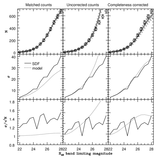
Figure 9: Comparison of the model to the SDF $R$ band. The model number counts have been calculated for an $\epsilon=3$ model. The left hand panels show the data matched exactly to the SDF number counts. The middle panels show a model with number counts calculated from number density surveys (see appendix A.1). The right hand panels show a model with number counts calculated from published surveys, but corrected for the incompleteness of the SDF observations. The top panels show the SDF mean number counts and the associated stand deviation, as open points with error bars. The grey area represents the predicted 1$\sigma$ uncertainty from the model, and the hatched area the 2$\sigma$ uncertainty. The middle panels show the increase in $\sigma$ as a function of limiting magnitude, and the bottom panels show the variation in $\sigma/\sqrt{N}$, i.e. the non-Poissonian component of the variance.

The models were also tested for in the $B$ and $i^{\prime}$ bands, and show very similar results. However, for the number counts at faint limiting $B$ and $i^{\prime}$ band magnitudes the model overcompensates for the incompleteness despite the fact that the incompleteness function is taken directly from the SDF observations of Kashikawa et al. (2004). Consequently the predicted uncertainties also fall below the measured values.

These discrepancies may be due in part to uncertainties in correcting for both the magnitude systems and the different filters used by the SDF and the collated number counts. Furthermore, the number counts are calculated from a cubic spline fit to an average of compiled number density surveys from the literature. The $B$ band SDF counts are systematically higher than the other surveys which reach faint magnitudes, and thus the average counts are already lower than the SDF counts before the incompleteness correction is applied. However, this still leaves the problem that the uncertainties in number counts are under-predicted by the model. We have shown in Figure  9 that the model will predict the uncertainties very accurately if the number counts as a function of magnitude are correct. Therefore it seems that the $B$ band SDF counts differ from the average counts by more than would be expected from cosmic variance. This is not to say the $B$ band SDF counts are wrong, but rather that there are systematic differences between published number count surveys that are larger than would be expected from cosmic variance, most likely resulting from uncertainty in correcting for incompleteness and subsequent extrapolation to the standard one square degree for which number densities are quoted. This is illustrated in Figure 10, which shows number density vs. magnitude. It is clear that the scatter dramatically increases at $B\mathrel{\hbox{\hbox to0.0pt{\hbox{\lower 4.0pt\hbox{$\sim$}}\hss}\hbox{$>$}}}25$, which is unlikely to be a real effect due to cosmic variance. In comparison the scatter in the $R$ band counts is much more uniform at faint magnitudes. The expected uncertainty due to cosmic variance is also shown in these plots. The grey curves show the expected cosmic variance from a survey of 1 deg²; the hatched curves show the expected cosmic variance from a survey of $1.17\times 10^{-3}$ deg² (the area of the Hubble Deep Field) extrapolated to 1 deg². Both simulations are assumed to be 100% complete, an additional small correction would be needed for incomplete surveys. The published number densities differ within cosmic variance at bright magnitudes but have a larger scatter at faint magnitudes. Whilst this is markedly more pronounced in the $B$ band it is also true in the $R$ band. The extra scatter at faint magnitudes can be attributed to systematic errors in accounting for the incompleteness of the surveys, or to systematic errors in consolidating the different magnitude systems of each survey. Note that an accurate number density is crucial to correctly calculate the associated uncertainties, and thus the average presented here may fail to achieve this if systematic errors really are present. We note though that the user is free to specify the number density exactly, and so may choose to rely on a particular survey of his or her own choice e.g. the Hubble Deep Fields, or to input a number density from his or her own survey.

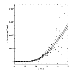
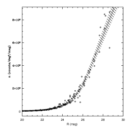
Figure 10: The number density of galaxies vs. magnitude, with $B$ on the left and $R$ on the right. The grey shaded curves show the number density and 1$\sigma$ uncertainty expected from cosmic variance. The hatched curves show the cosmic variance as measured in a survey with the the area of the Hubble Deep Field, and subsequently extrapolated to 1 deg².

3.2 General results

Table 1 shows the results for a selection of magnitude ranges and areas. These values were computed using the $\epsilon=3$ model, and assume 100% completeness at all magnitudes. The variances may be easily scaled to any number counts within the same magnitude range and area, assuming that the amplitude of the correlation function does not change, equation 5. After appropriate scaling, equation 4 may be used to estimate the completeness if the number of galaxies is unknown, e.g. if star-galaxy discrimination is not possible.

Table 1: Galaxy counts and standard deviations for a range of filters, magnitudes and areas. These values were computed using the $\epsilon=3$ model and assume 100% completeness at all magnitudes. The standard deviations may be scaled for incompleteness or higher number counts using equation 5.

	Counts and standard deviation within the given area
	$30^{\prime\prime}\times 30^{\prime\prime}$		$1^{\prime}\times 1^{\prime}$		$5^{\prime}\times 5^{\prime}$		$10^{\prime}\times 10^{\prime}$		$15^{\prime}\times 15^{\prime}$		$30^{\prime}\times 30^{\prime}$		$1^{\circ}\times 1^{\circ}$
Mag range	$N$	$\sigma$	$N$	$\sigma$	$N$	$\sigma$	$N$	$\sigma$	$N$	$\sigma$	$N$	$\sigma$	$N$	$\sigma$
$19\leq U\leq 21$	0	0	0	1	7	34	29	11	66	19	263	55	1050	160
$19\leq U\leq 23$	1	1	3	2	76	15	306	41	688	76	2750	220	11010	670
$19\leq U\leq 25$	7	3	27	6	669	58	2680	160	6020	310	24080	920	96300	2700
$19\leq U\leq 27$	30	6	121	15	3020	140	12100	410	27210	780	108900	2300	435400	7000
$15\leq B\leq 17$	0	0	0	0	0	0	0	1	0	1	2	2	6	6
$15\leq B\leq 19$	0	0	0	0	1	1	3	3	6	4	24	12	95	35
$15\leq B\leq 21$	0	0	0	0	6	3	22	8	50	14	199	40	800	120
$15\leq B\leq 23$	0	1	2	1	45	10	181	26	408	47	1630	140	6530	400
$15\leq B\leq 25$	4	2	18	5	449	45	1800	130	4040	240	16180	710	64700	2100
$15\leq B\leq 27$	23	6	93	13	2330	130	9310	370	20940	710	83800	2100	335100	6400
$15\leq B\leq 29$	70	10	282	24	7050	250	28190	720	63400	1400	253700	4100	1015000	12000
$15\leq R\leq 17$	0	0	0	0	0	1	2	1	4	2	14	5	58	14
$15\leq R\leq 19$	0	0	0	0	4	2	18	6	40	10	162	26	646	75
$15\leq R\leq 21$	0	1	1	1	33	8	131	20	295	36	1179	100	4720	290
$15\leq R\leq 23$	2	1	7	3	184	22	735	60	1650	110	6610	320	26450	950
$15\leq R\leq 25$	10	3	40	8	992	67	3970	190	8930	360	35700	1100	142900	3200
$15\leq R\leq 27$	44	8	175	19	4380	190	17510	540	39390	1000	157600	3100	630300	9300
$15\leq R\leq 28$	83	11	331	28	8260	290	33060	840	74400	1600	297500	4800	1190000	15000
$14\leq I\leq 16$	0	0	0	0	0	0	1	1	2	2	7	4	28	11
$14\leq I\leq 18$	0	0	0	0	4	2	14	6	32	11	129	31	514	89
$14\leq I\leq 20$	0	1	1	1	28	8	110	21	248	37	990	110	3970	320
$14\leq I\leq 22$	2	1	6	3	157	21	627	56	1410	100	5640	300	22560	900
$14\leq I\leq 24$	7	3	28	6	712	52	2850	140	6410	270	25630	790	102500	2400
$14\leq I\leq 26$	32	7	128	15	3190	140	12760	420	28710	790	114800	2400	459300	7100
$14\leq I\leq 28$	113	13	451	33	11280	340	45110	1010	101500	1900	406000	5700	1624000	17000
$13\leq K\leq 15$	0	0	0	0	1	1	5	3	11	5	42	14	169	39
$13\leq K\leq 17$	0	0	1	1	16	6	64	15	144	28	577	79	2310	230
$13\leq K\leq 19$	1	1	4	2	110	18	441	48	993	87	3970	260	15880	760
$13\leq K\leq 21$	5	3	22	5	543	44	2170	120	4890	230	19560	670	78200	2000
$13\leq K\leq 23$	20	5	81	11	2022	96	8090	270	18200	510	72800	1500	291200	4500

We have explicitly demonstrated the reliability of the $B$, $R$ and $I$ band predictions above, via comparison with the SDF. However, the $U$ and $K$ bands have not been checked since there are no sufficiently large and deep surveys to perform a satisfactory random counts-in-cells test. The $K$ band has good statistics on the number counts and the angular-correlation function, so there is no reason to suspect that the results will be very wrong but until they are checked against observations we cannot know for certain. The $U$ band is still more uncertain since the variation of $A$ with magnitude is unknown, and so the $B$ band function has been assumed, and normalised to the $U$ band.

4 Worked examples

4.1 NGC 300

We now provide a worked example to emphasise the importance of accurately determining the background galaxy counts in a given photometric band. Bland-Hawthorn et al. (2005) obtained deep observations of the stellar population in the outer disc of NGC 300, a late-type spiral in the Sculptor group. They used the Gemini Multi-object Spectrograph (GMOS) on the Gemini South 8m telescope in exceptional conditions (0.6” FWHM seeing). At a 3$\sigma$ point source detection threshold of $r^{\prime}=27.0$ mag, they were able to trace the stellar disc out to a radius of 24’, or $2.2\times R_{25}$ where $R_{25}$ is the 25 mag arcsec^-2 isophotal radius. This corresponds to about 10 scale lengths in this low-luminosity spiral ($M_{B}=-18.6$), or about 14.4 kpc at a distance of 2.0 Mpc.

These authors, and others (e.g. Ferguson et al. 2005; Irwin et al. 2005), demonstrate the profound importance of using star counts for tracing the outer reaches of galaxies. Bland-Hawthorn et al. (2005) reach an effective surface brightness of 30.5 mag arcsec^-2 (2$\sigma$) at 55% point source completeness which doubles the known radial extent of the optical disc. These levels are exceedingly faint in the sense that the equivalent surface brightness in $B$ or $V$ is about 32 mag arcsec^-2.

In the NGC 300 study, the authors found no evidence for truncation of the stellar disc such that the disc may extend even further. But this conclusion is sensitive to the assumed background galaxy counts. The disc can be forced to truncate at smaller radius if the background galaxy counts are close to or exceed 200 gals arcmin^-2. However, the authors found in favour of a lower background (130 gals arcmin^-2) by assuming that the outermost field is dominated by background galaxies.

Note that in order to statistically subtract background galaxies it is often necessary to observe “blank-sky” fields, for an equal amount of time as the field of interest. The java calculator obviates this expensive requirement (which in practice is not often met). Provided that the completeness of the target observations can be calculated, the deep galaxy surveys incorporated into the calculator can be used to subtract the contaminating galaxies and to estimate the associated error.

We now use GalaxyCount to predict the expected galaxy counts in $r^{\prime}$ for a 5.5’$\times$5.5’ field. This takes into account the seeing (0.6”), SNR=3$\sigma$, the telescope aperture (8m), total system throughput=39%, and the exposure time (8100s). For our values (in this case we use $R=r^{\prime}-0.2<26.8$, which is appropriate for stellar populations in the outer discs of galaxies, see Bland-Hawthorn et al. 2005), we determine 85 $\pm 11$ galaxies arcmin^-2, or 2560 $\pm$ 110 galaxies over the GMOS FOV, where the errors are 1$\sigma$, calculated using an $\epsilon=3$ model. This is equivalent to a total completeness of $\approx 56\%$ for $R\leq 26.8$ for galaxies as predicted by the calculator.

We now consider the impact of the background galaxy counts on the luminosity profile derived from the stellar counts. The primary aim of Bland-Hawthorn et al. (2005) was to obtain deep observations of the outer disc of NGC 300, and hence only a section of the disc was studied, located approximately 9kpc SW of the galaxy nucleus on the semi-major axis. Star counts were made in arcs of fixed width centred on the galaxy nucleus, thus the area of each segment is different. Consequently the uncertainty on the star counts and on the background galaxy counts will change as a function of radius.

Figure 11 reproduces the luminosity profile of NGC 300 star counts. There is no evidence for a truncation of the stellar disc; the star counts decline exponentially to the limits of the data, which is equal to about 10 scale lengths. This confirms the findings of Bland-Hawthorn et al. (2005), but with the added assurance that the errors introduced through the subtraction of an estimated or a theoretical number of background galaxies do not significantly affect the conclusions. Bland-Hawthorn et al. (2005) found they could generate a truncation of the disc if the background contains $\approx 220$ galaxies arcmin^-2, but this is ruled out at high significance.

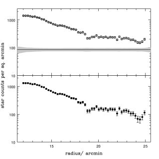
Figure 11: The luminosity profile of NGC 300. The top panel shows the raw counts as the open symbols, with the associated error (calculated as the square root of the counts), the solid line represents the expected contribution to the raw counts from background galaxies, and the shaded region represents the uncertainty on this number as predicted by GalaxyCount. In the bottom panel the closed symbols represent the corrected star counts, and the combined errors.

4.2 Galaxy cluster luminosity functions

Another application of GalaxyCount is the statistical removal of foreground and background galaxies from clusters in order to compute the properties of the cluster members. Here we provide an example of such use in the computation of the $b_{{\rm j}}$ band luminosity function (LF) of cluster Abell 2734. This cluster was selected from the two degree field galaxy redshift survey (2dFGRS) study of the cluster LF (De Propris et al. 2003), based on its high membership of 127 galaxies with the selection of De Propris et al. (2003). The cluster has a redshift of $cz=18646$ km s^-1 and velocity dispersion of $\sigma=1038$ km s^-1.

We have calculated the LF in three ways. First we select all galaxies within a box of 4Mpc centred on the cluster having redshifts within $\pm 3\sigma$ of the velocity dispersion. This yields an accurate catalogue of cluster members from which the cluster LF is computed. Secondly we count all galaxies within the 4Mpc box regardless of their redshifts, as if the redshifts were unknown. We then use GalaxyCount to estimate the number of interlopers as a function of magnitude and compute the LF based on these corrections. Finally we select offset fields around the cluster from which to measure the background galaxy counts to compare with the standard practice of statistical subtraction of foreground and background galaxies.

In order to use GalaxyCount to model the 2dFGRS counts the completeness limit must be accurately modelled. The 2dFGRS has a magnitude limit of $b_{\rm j}\approx 19.45$ mag, but varies slightly as a function of position. There is also a redshift completeness that is a function of magnitude. Colless et al. (2001) provide a model for the completeness function, and software is available from the 2dFGRS web pages to compute the necessary parameters to determine the final completeness as a function of magnitude. We match our sigmoid model to their completeness function, as shown in Figure 12. Finally we convert $B=b_{\rm j}+0.2$. It is worth re-emphasising that accurate completeness functions are crucial for the success of modelling expected counts with GalaxyCount since the number counts at faint magnitudes are so dominant. Note though that accurate completeness functions can be readily computed from the imaging data in question.

Figure 12: The 2dFGRS completeness as a function of magnitude at the position of A2734 is shown by the solid line. The dotted line is our sigmoid representation.

The offset fields were chosen at 1 and 2 degree displacements in RA and dec around cluster centre giving 24 fields in total. Computing the LFs for a large number of offset fields allows us to determine the relative merits of using GalaxyCount against using offset fields, since different offset fields can give very different results. Note that there are two methods in which the offset LFs may be computed: by using the total raw counts in the cluster and offset fields, or by counting only those galaxies for which redshifts are known. The former method mimics how the technique would usually be employed in standard observational practice, since statistical subtraction is only performed in the absence of spectroscopic redshifts, hence these are the results we report. The latter method accounts for the redshift incompleteness of the spectroscopic LF. Since incompleteness has been accounted for in the GalaxyCount derived model we also tested the latter technique. The results were not significantly different since the magnitude limit of the 2dF input catalogue is bright enough that observations are not much affected by the magnitude dependent redshift incompleteness.

The LFs were computed following the method described in Ellis & Jones (2004). Schechter (1976) functions were fit for all galaxies $b_{{\rm j}}\leq 19.4384$, i.e. the magnitude limit of the 2dFGRS at this position, through minimisation of Cash (1979) statistic. The resulting fits to the characteristic magnitude, $M^{*}$, and the faint end slope, $\alpha$, are shown in Figure 13. The GalaxyCount derived Schechter function is inside the 68 per cent confidence limit of the best fitting spectroscopic results. Only one offset field is far inside the 68 per cent confidence ellipse, with another 5 offset fields just inside, and another 18 further out. Thus we expect GalaxyCount to be more reliable than an offset field $\sim$75 per cent of the time. Forty per cent of the offset fields lie outside the 90 per cent confidence limits. Note that in general it is very difficult to get time allocation committees to grant more than a single offset field per cluster, and there is no way of knowing a posteriori whether a ‘good’ offset field has been observed.

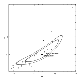
Figure 13: The best fitting Schechter functions as described in the text. The contours show the 68 and 90 per cent confidence limits of the spectroscopic LF.

Another way of comparing the results is calculate the reduced $\chi^{2}$ difference between the statistically subtracted LFs and the spectroscopic LF. These results are presented in Figure 14, which shows a histogram of the $\tilde{\chi}^{2}$ for the 24 offset fields, with the value for GalaxyCount overlaid. GalaxyCount is placed in the upper 25 per cent of the offset fields, and occurs near the peak of the distribution, i.e. it accurately reflects the expected average result that would be obtained from subtracting a large number of offset fields.

Figure 14: Histogram of the $\tilde{\chi}^{2}$ difference between the statistically subtracted LFs and the spectroscopic LF. The value for GalaxyCount is overlaid and is in the upper 25 per cent of the offset fields.

Thus GalaxyCount provides an accurate and efficient way to estimate the contribution of foreground and background galaxies to cluster LFs. In many cases expensive spectroscopic follow-up or off-source background observations may be by-passed and replaced with background estimates from GalaxyCount combined with an accurate determination of the completeness of the observations.

4.3 Comparison to the Hubble deep fields

The Hubble Deep Field North (HDF-N) has higher galaxy number counts than the Hubble Deep Field South (HDF-S, Metcalfe et al. 2001). Figure 15 compares the difference between the two fields to the expected standard deviation as predicted by GalaxyCount, with the number counts matched to the average of HDF-N and S. The two fields are within 1$\sigma$ of each other when using the $\epsilon=3$ model. Thus it seems that cosmic variance is enough to account for the difference between the two fields. GalaxyCount will be updated to include counts from the Hubble Ultra Deep Field when these become available.

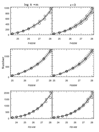
Figure 15: The difference between the Hubble deep fields N (squares) and S (circles), compared to the expected standard deviation (1$\sigma$=grey shaded area, 2$\sigma$=hatched area).

5 Discussion

5.1 General results

We have presented a model to predict the galaxy counts, variances and completeness of observations as a function of magnitude, waveband and area. The models have been compared to observed number counts and densities calculated using the SDF. It was found that the model will accurately predict the standard deviation on a given number of galaxies. Hence for any application for which the number of galaxies is known a priori the calculator should accurately determine the appropriate cosmic variance.

For observations (such as star counts) for which the number of galaxies is not known, more caution must be exercised in using the models. The derived standard deviation is strongly dependent on the number of galaxies. However at faint magnitudes an accurate estimate of the number counts can be difficult to determine since the scatter in values published in the literature varies more than the predicted cosmic variance (for example in the $B$ band). The systematic errors introduced into the number counts are propagated into the resulting standard deviation. In practice this means that the statistical subtraction of galaxy counts may be dominated by systematic uncertainties rather than cosmic variance in the $B$ band. However, for brighter magnitudes where completeness is not an issue the predicted number counts are reliable.

The problem may be alleviated with future, more precise determinations of the faint end number counts. Until such data is available it is up to the user to choose wisely the number counts which he or she wishes to use and to be aware of the possible systematic uncertainties introduced at faint magnitudes.

The $\epsilon=3$ model was found to predict the standard deviation accurately. This model has a monotonic decrease in log $A$ with magnitude at bright magnitudes, but flattens off at faint magnitudes. Such a trend has previously been observed in several studies (e.g. Brainerd & Smail 1998; Postman et al. 1998), although many other studies find no such trend (e.g. McCracken et al. 2001; Wilson 2003; Coil et al. 2004). Figure 6 shows that for the data compiled from the literature a simple monotonic model seems to be a better fit. However, we are extrapolating $A$ to fainter magnitudes than the measurements, thus it may be that some flattening is required at very faint magnitudes, beyond the limit of the data. Note that the counts at faint magnitudes dominate the statistics, thus we are testing the currently unknown functional form of the relation at these magnitudes.

An $\epsilon=3$ model implies a strong evolution in the clustering of galaxies since $z=1$. However, we caution that the physical interpretation of the model should not be taken too literally, since the models do not fit $A$ at all magnitudes, rather the model was used allow a flattening of $A$ at the faint end. Other studies have reported that a high value of $\epsilon$ is required to fit the faint end of the $A$ scaling relation (McCracken et al. 2000b; McCracken et al. 2001; Coil et al. 2004), but note that these models cannot fit both the bright and the faint ends of the relation simultaneously. A precise determination of the value of $A$ at faint magnitudes awaits future measurements. We remind the reader, however, that the models used in GalaxyCount can accurately reproduce the measured standard deviation of galaxy counts in the SDF, despite the uncertainty in the precise functional form of $A$.

GalaxyCount has a demonstrated practical use as shown by our reanalyses of the star counts in NGC 300, and the LF of Abell 2734. The calculator will prove useful for any observations subject to an unknown background or foreground of galaxies, and in many cases should obviate the need for expensive ‘blank-sky’ observations.

5.2 When is cosmic variance significant?

An important consideration is when does cosmic variance need to be accounted for? In some circumstances the Poissonian component of the variance will dominate over cosmic variance due to clustering, whereas in others the excess uncertainty will be very important. This has been addressed throughout the paper by presenting $\sigma/\sqrt{N}$, the factor by which the total standard deviation is greater than the Poissonian standard deviation. This factor increases with the area and depth of the survey (see equation 1). We show the form of the dependence in Figure 16 for the $R$ band predictions as calculated in Table 1.

Figure 16: The factor by which the total standard deviation dominates over the Poissonian error, $\sigma/\sqrt{N}$, as a function of $R$ band limiting magnitude for various field sizes (labelled in the plot in units of square arcminutes).

The non-Possonian contribution quickly becomes important as the surveyed area or the depth of the survey increases; the exact point at which it becomes non-negligible depends on the combination of these variables and the accuracy needed. For example for a survey reaching a limiting magnitude of $R\leq 26$ mag, Poissonian variance will be within a factor of 2 of the true variance only if the area is $\mathrel{\hbox{\hbox to0.0pt{\hbox{\lower 4.0pt\hbox{$\sim$}}\hss}\hbox{$<$}}}10$ arcmin². Other conditions can easily be tested using the values given in Table 1.

5.3 Future work

GalaxyCount will be kept up to date with the inclusion of the latest number densities and angular correlation functions as they are published, including the Hubble Ultra Deep Field number counts. In addition it will be extended to include predictions for specific targets such as Ly-$\alpha$ sources at high $z$, specific observing conditions such as HST/ JWST observations with a fixed point spread function, and ground-based AO-corrected observations, etc. An extension is also planned to include predictions of star-counts as a function of co-ordinates, magnitude and FOV. All future upgrades will be available from the web-site.

Appendix A Sources of data for number counts and angular correlation functions

A.1 Number density

The expected number counts of galaxies in the $UBRIK$ bands has been calculated using a large number of published surveys of galaxy number density, which have been compiled from the following papers: $U$ band, Koo (1986), Guhathakurta et al. (1990), Maddox et al. (1990), Songaila et al. (1990), Jones et al. (1991), Arnouts et al. (2001), Metcalfe et al. (2001), Capak et al. (2004); $B$ band, Kron (1978), Jarvis & Tyson (1981), Koo (1986), Peterson et al. (1986), Stevenson et al. (1986), Tyson (1988), Heydon-Dumbleton et al. (1989), Jones et al. (1991), Lilly et al. (1991), Metcalfe et al. (1991), Metcalfe et al. (1995), Bertin & Dennefeld (1997), Metcalfe et al. (1998), Arnouts et al. (1999), Arnouts et al. (2001), Huang et al. (2001), Kümmel & Wagner (2001), Metcalfe et al. (2001), Yasuda et al. (2001), Liske et al. (2003), Capak et al. (2004), as well as the Revised Shapley Ames and the Zwicky cat. both from the Durham galaxy counts web pages; $R$ band, Couch & Newell (1984), Hall & Mackay (1984), Infante et al. (1986), Koo (1986), Stevenson et al. (1986), Yee & Green (1987), Tyson (1988), Jones et al. (1991), Metcalfe et al. (1991), Picard (1991), Couch et al. (1993), Steidel & Hamilton (1993), Driver et al. (1994), Metcalfe et al. (1995), Smail et al. (1995), Bertin & Dennefeld (1997), Hogg et al. (1997), Metcalfe et al. (1998), Arnouts et al. (1999), Arnouts et al. (2001), Huang et al. (2001), Kümmel & Wagner (2001), Metcalfe et al. (2001), Capak et al. (2004); $I$ band, Hall & Mackay (1984), Koo (1986), Tyson (1988), Lilly et al. (1991), Driver et al. (1994), Casertano et al. (1995), Driver et al. (1995), Glazebrook et al. (1995), Le Fevre et al. (1995), Smail et al. (1995), Mamon (1998), Postman et al. (1998), Arnouts et al. (1999), Arnouts et al. (2001), Metcalfe et al. (2001), Yasuda et al. (2001), Capak et al. (2004); $K$ band, Mobasher et al. (1986), Gardner et al. (1993), Soifer et al. (1994), Djorgovski et al. (1995), Glazebrook et al. (1995), McLeod et al. (1995), Gardner et al. (1996), Huang et al. (1997), Moustakas et al. (1997), Saracco et al. (1997), Bershady et al. (1998), Szokoly et al. (1998), Mamon (1998), McCracken et al. (2000a), Väisänen et al. (2000), Martini (2001), Huang et al. (2001), Kochanek et al. (2001), Kümmel & Wagner (2001), Maihara et al. (2001), Metcalfe et al. (2001), Saracco et al. (2001), Vandame et al. (2001, preprint, astro-ph/0102300), Minowa et al. (2005), and the 2MASS $K$s counts from the Durham galaxy counts web pages. The majority of the above number counts were retrieved from the Durham galaxy counts web pages.

A.2 Amplitude of the angular correlation function

Measurements of the angular correlation function were taken from: $U$ band, Efstathiou et al. (1991); $B$ band, Koo & Szalay (1984), Efstathiou et al. (1991), Roche et al. (1993); $R$ band, Efstathiou et al. (1991), Roche et al. (1993), Brainerd et al. (1995), Hudon & Lilly (1996), Villumsen et al. (1997), Woods & Fahlman (1997), Roche & Eales (1999), Connolly et al. (2002); $I$ band, Efstathiou et al. (1991), Postman et al. (1998), Cabanac et al. (2000), Wilson (2003), Coil et al. (2004); $K$ band, Baugh et al. (1996), Carlberg et al. (1997), Roche et al. (1999), Kümmel & Wagner (2000), Maller et al. (2005).

References

- Arnouts et al. (1999) Arnouts, S., D’Odorico, S., Cristiani, S., Zaggia, S., Fontana, A., Giallongo, E. 1999, A&A, 341, 641
- Arnouts et al. (2001) Arnouts, S., et al. 2001, A&A, 379, 740
- Baugh et al. (1996) Baugh, C. M., Gardner, J. P., Frenk, C. S., Sharples, R. M. 1996, MNRAS, 283, L15
- Bershady et al. (1998) Bershady, M. A., Lowenthal, J. D., Koo, D. C. 1998, ApJ, 505, 50
- Bertin & Arnouts (1996) Bertin, E., Arnouts, S. 1996, A&AS, 117, 393
- Bertin & Dennefeld (1997) Bertin, E., Dennefeld, M. 1997, A&A, 317, 43
- Bland-Hawthorn (2006) Bland-Hawthorn, J. 2006, New Astronomy Reviews, 50, 75
- Bland-Hawthorn et al. (2005) Bland-Hawthorn, J., Vlajić, M., Freeman, K. C., Draine, B. T. 2005, ApJ, 629, 239
- Brainerd & Smail (1998) Brainerd, T. G., Smail, I. 1998, ApJ, 494, L137
- Brainerd et al. (1995) Brainerd, T. G., Smail, I., Mould, J. 1995, MNRAS, 275, 781
- Bruzual & Charlot (2003) Bruzual, G., Charlot, S. 2003, MNRAS, 344, 1000
- Cabanac et al. (2000) Cabanac, R. A., de Lapparent, V., Hickson, P. 2000, A&A, 364, 349
- Capak et al. (2004) Capak, P., et al. 2004, AJ, 127, 180
- Carlberg et al. (1997) Carlberg, R. G., Cowie, L. L., Songaila, A., Hu, E. M. 1997, ApJ, 484, 538
- Casertano et al. (1995) Casertano, S., Ratnatunga, K. U., Griffiths, R. E., Im, M., Neuschaefer, L. W., Ostrander, E. J., Windhorst, R. A. 1995, ApJ, 453, 599
- Cash (1979) Cash, W. 1979, ApJ, 228, 939
- Coil et al. (2004) Coil, A. L., Newman, J. A., Kaiser, N., Davis, M., Ma, C.-P., Kocevski, D. D., Koo, D. C. 2004, ApJ, 617, 765
- Colless et al. (2001) Colless, M., et al. 2001, MNRAS, 328, 1039
- Connolly et al. (2002) Connolly, A. J., et al. 2002, ApJ, 579, 42
- Couch et al. (1993) Couch, W. J., Jurcevic, J. S., Boyle, B. J. 1993, MNRAS, 260, 241
- Couch & Newell (1984) Couch, W. J., Newell, E. B. 1984, ApJS, 56, 143
- Cresci et al. (2006) Cresci, G., Davies, R. I., Baker, A. J., Mannucci, F., Lehnert, M. D., Totani, T., Minowa, Y. 2006, A&A, 458, 385
- Cuby et al. (2007) Cuby, J.-G., Hibon, P., Lidman, C., Le Fèvre, O., Gilmozzi, R., Moorwood, A., van der Werf, P. 2007, A&A, 461, 911
- De Propris et al. (2003) De Propris, R., et al. 2003, MNRAS, 342, 725
- Djorgovski et al. (1995) Djorgovski, S., et al. 1995, ApJ, 438, L13
- Driver et al. (1994) Driver, S. P., Phillipps, S., Davies, J. I., Morgan, I., Disney, M. J. 1994, MNRAS, 268, 393
- Driver et al. (1995) Driver, S. P., Windhorst, R. A., Ostrander, E. J., Keel, W. C., Griffiths, R. E., Ratnatunga, K. U. 1995, ApJ, 449, L23
- Efstathiou et al. (1991) Efstathiou, G., Bernstein, G., Tyson, J. A., Katz, N., Guhathakurta, P. 1991, ApJ, 380, L47
- Ellis & Jones (2004) Ellis, S. C., Jones, L. R. 2004, MNRAS, 348, 165
- Ferguson et al. (2005) Ferguson, A. M. N., Johnson, R. A., Faria, D. C., Irwin, M. J., Ibata, R. A., Johnston, K. V., Lewis, G. F., Tanvir, N. R. 2005, ApJ, 622, L109
- Fukugita et al. (1996) Fukugita, M., Ichikawa, T., Gunn, J. E., Doi, M., Shimasaku, K., Schneider, D. P. 1996, AJ, 111, 1748
- Gardner et al. (1993) Gardner, J. P., Cowie, L. L., Wainscoat, R. J. 1993, ApJ, 415, L9
- Gardner et al. (1996) Gardner, J. P., Sharples, R. M., Carrasco, B. E., Frenk, C. S. 1996, MNRAS, 282, L1
- Glazebrook et al. (1995) Glazebrook, K., Ellis, R., Santiago, B., Griffiths, R. 1995, MNRAS, 275, L19
- Groth & Peebles (1977) Groth, E. J., Peebles, P. J. E. 1977, ApJ, 217, 385
- Guhathakurta et al. (1990) Guhathakurta, P., Tyson, J. A., Majewski, S. R. 1990, ApJ, 357, L9
- Hall & Mackay (1984) Hall, P., Mackay, C. D. 1984, MNRAS, 210, 979
- Heydon-Dumbleton et al. (1989) Heydon-Dumbleton, N. H., Collins, C. A., MacGillivray, H. T. 1989, MNRAS, 238, 379
- Hogg et al. (1997) Hogg, D. W., Pahre, M. A., McCarthy, J. K., Cohen, J. G., Blandford, R., Smail, I., Soifer, B. T. 1997, MNRAS, 288, 404
- Hook et al. (2004) Hook, I. M., Jørgensen, I., Allington-Smith, J. R., Davies, R. L., Metcalfe, N., Murowinski, R. G., Crampton, D. 2004, PASP, 116, 425
- Huang et al. (1997) Huang, J.-S., Cowie, L. L., Gardner, J. P., Hu, E. M., Songaila, A., Wainscoat, R. J. 1997, ApJ, 476, 12
- Huang et al. (2001) Huang, J.-S., et al. 2001, A&A, 368, 787
- Hudon & Lilly (1996) Hudon, J. D., Lilly, S. J. 1996, ApJ, 469, 519
- Infante et al. (1986) Infante, L., Pritchet, C., Quintana, H. 1986, AJ, 91, 217
- Irwin et al. (2005) Irwin, M. J., Ferguson, A. M. N., Ibata, R. A., Lewis, G. F., Tanvir, N. R. 2005, ApJ, 628, L105
- Jarvis & Tyson (1981) Jarvis, J. F., Tyson, J. A. 1981, AJ, 86, 476
- Jones et al. (1991) Jones, L. R., Fong, R., Shanks, T., Ellis, R. S., Peterson, B. A. 1991, MNRAS, 249, 481
- Kümmel & Wagner (2001) Kümmel, M. W., Wagner, S. J. 2001, A&A, 370, 384
- Kashikawa et al. (2004) Kashikawa, N., et al. 2004, PASJ, 56, 1011
- Kochanek et al. (2001) Kochanek, C. S., et al. 2001, ApJ, 560, 566
- Koo (1986) Koo, D. C. 1986, ApJ, 311, 651
- Koo & Szalay (1984) Koo, D. C., Szalay, A. S. 1984, ApJ, 282, 390
- Kron (1980) Kron, R. 1980, ApJS, 43, 305
- Kron (1978) Kron, R. G. 1978, Ph.D. Thesis
- Kümmel & Wagner (2000) Kümmel, M. W., Wagner, S. J. 2000, A&A, 353, 867
- Le Fevre et al. (1995) Le Fevre, O., Crampton, D., Lilly, S. J., Hammer, F., Tresse, L. 1995, ApJ, 455, 60
- Lilly et al. (1991) Lilly, S. J., Cowie, L. L., Gardner, J. P. 1991, ApJ, 369, 79
- Liske et al. (2003) Liske, J., Lemon, D. J., Driver, S. P., Cross, N. J. G., Couch, W. J. 2003, MNRAS, 344, 307
- Maddox et al. (1990) Maddox, S. J., Sutherland, W. J., Efstathiou, G., Loveday, J., Peterson, B. A. 1990, MNRAS, 247, 1
- Maihara et al. (2001) Maihara, T., et al. 2001, PASJ, 53, 25
- Maller et al. (2005) Maller, A. H., McIntosh, D. H., Katz, N., Weinberg, M. D. 2005, ApJ, 619, 147
- Mamon (1998) Mamon, G. A. 1998, in Wide Field Surveys in Cosmology, 14th IAP meeting held May 26-30, 1998, Paris. Publisher: Editions Frontieres. ISBN: 2-8 6332-241-9, p. 323., 323
- Martini (2001) Martini, P. 2001, AJ, 121, 598
- McCracken et al. (2001) McCracken, H. J., Le Fèvre, O., Brodwin, M., Foucaud, S., Lilly, S. J., Crampton, D., Mellier, Y. 2001, A&A, 376, 756
- McCracken et al. (2000a) McCracken, H. J., Metcalfe, N., Shanks, T., Campos, A., Gardner, J. P., Fong, R. 2000a, MNRAS, 311, 707
- McCracken et al. (2000b) McCracken, H. J., Shanks, T., Metcalfe, N., Fong, R., Campos, A. 2000b, MNRAS, 318, 913
- McLeod et al. (1995) McLeod, B. A., Bernstein, G. M., Rieke, M. J., Tollestrup, E. V., Fazio, G. G. 1995, ApJS, 96, 117
- Metcalfe et al. (1998) Metcalfe, N., Ratcliffe, A., Shanks, T., Fong, R. 1998, MNRAS, 294, 147
- Metcalfe et al. (2001) Metcalfe, N., Shanks, T., Campos, A., McCracken, H. J., Fong, R. 2001, MNRAS, 323, 795
- Metcalfe et al. (1991) Metcalfe, N., Shanks, T., Fong, R., Jones, L. R. 1991, MNRAS, 249, 498
- Metcalfe et al. (1995) Metcalfe, N., Shanks, T., Fong, R., Roche, N. 1995, MNRAS, 273, 257
- Minowa et al. (2005) Minowa, Y., et al. 2005, ApJ, in press
- Miyazaki et al. (2002) Miyazaki, S., et al. 2002, PASJ, 54, 833
- Mobasher et al. (1986) Mobasher, B., Ellis, R. S., Sharples, R. M. 1986, MNRAS, 223, 11
- Motohara et al. (2002) Motohara, K., et al. 2002, PASJ, 54, 315
- Moustakas et al. (1997) Moustakas, L. A., Davis, M., Graham, J. R., Silk, J., Peterson, B. A., Yoshii, Y. 1997, ApJ, 475, 445
- Ouchi et al. (2005) Ouchi, M., et al. 2005, ApJ, 635, L117
- Peebles (1975) Peebles, P. J. E. 1975, ApJ, 196, 647
- Peebles (1980) Peebles, P. J. E. 1980, The Large-Scale Structure of the Universe. (Princeton University Press, Princeton, NJ)
- Peterson et al. (1986) Peterson, B. A., Ellis, R. S., Efstathiou, G., Shanks, T., Bean, A. J., Fong, R., Zen-Long, Z. 1986, MNRAS, 221, 233
- Petrosian (1976) Petrosian, V. 1976, ApJ, 209, L1
- Picard (1991) Picard, A. 1991, AJ, 102, 445
- Postman et al. (1998) Postman, M., Lauer, T. R., Szapudi, I., Oegerle, W. 1998, ApJ, 506, 33
- Robin et al. (2003) Robin, A. C., Reylé, C., Derrière, S., Picaud, S. 2003, A&A, 409, 523
- Roche & Eales (1999) Roche, N., Eales, S. A. 1999, MNRAS, 307, 703
- Roche et al. (1999) Roche, N., Eales, S. A., Hippelein, H., Willott, C. J. 1999, MNRAS, 306, 538
- Roche et al. (1993) Roche, N., Shanks, T., Metcalfe, N., Fong, R. 1993, MNRAS, 263, 360
- Saracco et al. (2001) Saracco, P., Giallongo, E., Cristiani, S., D’Odorico, S., Fontana, A., Iovino, A., Poli, F., Vanzella, E. 2001, A&A, 375, 1
- Saracco et al. (1997) Saracco, P., Iovino, A., Garilli, B., Maccagni, D., Chincarini, G. 1997, AJ, 114, 887
- Schechter (1976) Schechter, P. 1976, ApJ, 203, 297
- Smail et al. (1995) Smail, I., Hogg, D. W., Yan, L., Cohen, J. G. 1995, ApJ, 449, L105
- Soifer et al. (1994) Soifer, B. T., et al. 1994, ApJ, 420, L1
- Songaila et al. (1990) Songaila, A., Cowie, L. L., Lilly, S. J. 1990, ApJ, 348, 371
- Steidel & Hamilton (1993) Steidel, C. C., Hamilton, D. 1993, AJ, 105, 2017
- Stevenson et al. (1986) Stevenson, P. R. F., Shanks, T., Fong, R. 1986, ASP Conf. Ser., Spectral Evolution of Galaxies, eds. Chiosi, C. and Renzini, A., 146, 439
- Szokoly et al. (1998) Szokoly, G. P., Subbarao, M. U., Connolly, A. J., Mobasher, B. 1998, ApJ, 492, 452
- Tyson (1988) Tyson, J. A. 1988, AJ, 96, 1
- Väisänen et al. (2000) Väisänen, P., Tollestrup, E. V., Willner, S. P., Cohen, M. 2000, ApJ, 540, 593
- Villumsen et al. (1997) Villumsen, J. V., Freudling, W., da Costa, L. N. 1997, ApJ, 481, 578
- Wilson (2003) Wilson, G. 2003, ApJ, 585, 191
- Woods & Fahlman (1997) Woods, D., Fahlman, G. G. 1997, ApJ, 490, 11
- Yasuda et al. (2001) Yasuda, N., et al. 2001, AJ, 122, 1104
- Yee & Green (1987) Yee, H. K. C., Green, R. F. 1987, ApJ, 319, 28