A Spectroscopic Survey of Faint Quasars in the SDSS Deep Stripe: I. Preliminary Results from the Co-added Catalog

Abstract

In this paper we present the first results of a deep spectroscopic survey of faint quasars in the Sloan Digital Sky Survey (SDSS) Southern Survey, a deep survey carried out by repeatedly imaging a 270 deg² area. Quasar candidates were selected from the deep data with good completeness over $0<z<5$, and 2 to 3 magnitudes fainter than the SDSS main survey. Spectroscopic follow-up was carried out on the 6.5m MMT with Hectospec. The preliminary sample of this SDSS faint quasar survey (hereafter SFQS) covers $\sim 3.9$ deg², contains 414 quasars, and reaches $g=22.5$. The overall selection efficiency is $\sim$ 66% ($\sim$ 80% at $g<21.5$); the efficiency in the most difficult redshift range ($2<z<3$) is better than 40%. We use the $1/V_{a}$ method to derive a binned estimate of the quasar luminosity function (QLF) and model the QLF using maximum likelihood analysis. The best model fits confirm previous results showing that the QLF has steep slopes at the bright end and much flatter slopes ($-1.25$ at $z\lesssim 2.0$ and $-1.55$ at $z\gtrsim 2.0$) at the faint end, indicating a break in the QLF slope. Using a luminosity-dependent density evolution model, we find that the quasar density at $M_{g}<-22.5$ peaks at $z\sim 2$, which is later in cosmic time than the peak of $z\sim 2.5$ found from surveys of more luminous objects. The SFQS QLF is consistent with the results of the 2dF QSO Redshift Survey, the SDSS, and the 2dF-SDSS LRG and QSO Survey, but probes fainter quasars. We plan to obtain more quasars from future observations and establish a complete faint quasar sample with more than 1000 objects over 10 deg².

1 Introduction

One of the most important properties of quasars is their strong evolution with cosmic time. The quasar luminosity function (QLF) is thus of particular importance in understanding quasar formation and evolution and exploring physical models of quasars. It has been shown that quasar activity and the formation processes of galaxies and supermassive black holes (SMBHs) are closely correlated (e.g. Kauffmann & Haehnelt, 2000; Wyithe & Loeb, 2003; Hopkins et al., 2005; Croton et al., 2006), so the QLF is essential to study galaxy formation, the accretion history of SMBHs during the active quasar phase, and its relation to galaxy evolution. Quasars are strong X-ray sources, thus the QLF can provide important constraints on the quasar contribution to the X-ray and ultraviolet background radiation (e.g. Koo & Kron, 1988; Boyle & Terlevich, 1998; Mushotzky et al., 2000; Worsley et al., 2005). The QLF is also useful for understanding the spatial clustering of quasars and its relation to quasar life times (e.g. Martini & Weinberg, 2001).

The differential QLF is defined as the density of quasars per unit comoving volume and unit luminosity interval as a function of luminosity and redshift. If the redshift and luminosity dependence is separable, the QLF can be modeled in terms of pure density evolution (PDE), pure luminosity evolution (PLE), or a combination of the two forms. Earlier work found that there was a strong decline of quasar activity from $z\sim 2$ to the present universe, and a model with a single power-law shape provided good fits to the observed QLF for $z<2$ at the bright end (Marshall et al., 1983, 1984; Marshall, 1985). When more faint quasars were discovered, a break was found in the luminosity function (e.g. Koo & Kron, 1988; Boyle, Shanks, & Peterson, 1988), and the shape of QLF was modeled by a double power-law form with a steep bright end and a much flatter faint end. In this double power-law model, luminosities evolve as PLE, and density evolution is not necessary (e.g. Boyle, Shanks, & Peterson, 1988). Some studies cast doubt on this claim, however. First, the existence of the break in the QLF slope is not obvious (e.g. Hawkins & Véron, 1995; Goldschmidt & Miller, 1998; Wisotzki, 2000; Wolf et al., 2003). Second, it was found that the PLE model was not sufficient to describe the quasar evolution at $z<2$ (e.g. Hewett, Foltz, & Chaffee, 1993; La Franca & Cristiani, 1997; Goldschmidt & Miller, 1998; Wisotzki, 2000).

The density of luminous quasars reaches a maximum at $2<z<3$ (hereafter referred to as the mid-$z$ range), and drops rapidly toward higher redshift (e.g. Pei, 1995). The high-$z$ ($z>3$) QLF has been explored only for bright quasars (e.g. Warren, Hewett, & Osmer, 1994; Kennefick, Djorgovski, & De Carvalho, 1995; Schmidt, Schneider, & Gunn, 1995; Fan et al., 2001b). At $z\sim 4$, the QLF was fitted by a single power-law form with an exponential decline in density with redshift (Schmidt, Schneider, & Gunn, 1995; Fan et al., 2001b), and its slope is much flatter than the bright-end slope of the QLF at $z<3$. This indicates that, at high redshift, the shape of the QLF evolves with redshift as well (Fan et al., 2001b). However, a large sample of high-$z$ quasars is needed to prove this claim.

One of the largest homogeneous samples of low-$z$ quasars comes from the 2dF QSO Redshift Survey and 6dF QSO Redshift Survey (hereafter 2QZ; Boyle et al., 2000; Croom et al., 2004). The 2QZ survey includes 25,000 quasars, and covers a redshift range of $0.4<z<2.1$ and a magnitude range of $16<b_{J}<20.85$. The QLF derived from the 2QZ can be well fitted by a double power-law form with a steep slope at the bright end and a flatter slope at the faint end, showing a break in the QLF. The evolution is well described by the PLE. The Sloan Digital Sky Survey (SDSS; York et al., 2000) is collecting the largest spectroscopic samples of galaxies and quasars to date. The SDSS main survey covers a large redshift range from $z=0$ to $z>5$, however, it only selects bright objects: it targets quasars with $i<19.1$ at $z\lesssim 3$ and $i<20.2$ at $z\gtrsim 3$ (Richards et al., 2002). The QLF derived from SDSS Data Release Three (DR3; Schneider et al., 2005) shows some curvature at the faint end, but the survey does not probe faint enough to test the existence of the break (Richards et al., 2006). The best fit model of the SDSS-DR3 QLF shows, for the first time in a single large redshift range, the flattening of the QLF slope with increasing redshift. Selecting $g<21.85$ and $z<2.5$ quasar candidates from SDSS imaging and spectroscopically observing them with the 2dF instrument, the 2dF-SDSS LRG and QSO Survey (2SLAQ) probes deeper than either the SDSS or the 2QZ (Richards et al., 2005). The QLF of the 2SLAQ is consistent with the 2QZ QLF from Boyle et al. (2000), but has a steeper faint-end slope than that from Croom et al. (2004).

Despite the investigations described above, the optical QLF over both a large redshift range and a large luminosity range is far from well established. First, the faint-end slope of the QLF is still uncertain. Most wide-field surveys, including the SDSS, are shallow and can only sample the luminous quasars. Although the 2SLAQ survey probed to $g=21.85$, it only covers the low-$z$ range ($z\lesssim 2.2$). Furthermore, the existence of the break in the QLF slope is uncertain, and different surveys give different slopes at the faint end (e.g. Wolf et al., 2003; Croom et al., 2004; Richards et al., 2005). Second, it is unclear whether PLE is sufficient to describe quasar evolution at low redshift. Third, the high-$z$ ($z>3$) QLF has not been well established, especially at the faint end. In addition, the density of luminous quasars peaks between $z=2$ and $z=3$, yet the colors of quasars with $2.2<z<3$ are similar to those of A and F stars, making selection of these objects difficult (Fan, 1999; Richards et al., 2002, 2006). X-ray and infrared surveys provide other ways to determine the QLF of both type I and type II AGNs (e.g. Ueda et al., 2003; Barger et al., 2005; Hasinger, Miyaji, & Schmidt, 2005; Brown et al., 2006). These studies have shown that a substantial fraction of AGNs are optically obscured at low luminosities. Barger et al. (2005) found a downturn at the faint end of the hard X-ray luminosity function for type I AGN, but current optically-selected quasar samples are not sufficiently faint to probe this downturn, if it exists.

To probe these issues, we need a large, homogeneous, faint quasar sample. This sample should be deep enough to study quasar behavior at the faint end, and large enough to provide good statistics. The sample should also span a large redshift range, straddling the peak of quasar activity. All these require a wide-field spectroscopic survey of faint quasars selected from deep multi-color imaging data. Such data are provided by the SDSS Southern Survey, a deep survey based on repeated imaging of the Fall Celestial Equatorial Stripe in the Southern Galactic Cap (SGC). The SGC imaging data, when co-added, reach more than two magnitudes deeper than does the SDSS main survey, allowing efficient selection of much fainter quasar candidates. The goal of the SDSS faint quasar survey (SFQS) is to obtain more than 1000 faint quasars from 10 deg² of the SDSS deep stripe. This paper presents the first results of the SFQS, in an area of $\sim 3.9$ deg². The spectroscopic observations were performed on MMT/Hectospec (Fabricant et al., 1998). The preliminary faint quasar sample reaches $g=22.5$, and fills in the crucial gap between large-area, shallow surveys such as the SDSS and 2QZ, and deep, pencil beam surveys such as the $Chandra$ Deep Field (CDF) survey (e.g. Barger et al., 2005) and COMBO-17 survey (e.g. Wolf et al., 2003).

In $\S$ 2 of this paper, we introduce the SDSS deep imaging survey and the color selections of faint quasars from the deep data. In $\S$ 3, we describe follow-up spectroscopic observations on MMT/Hectospec, and present the preliminary sample of the SFQS. We derive the QLF for the SFQS sample in $\S$ 4, and compare our results to other surveys in $\S$ 5. Throughout the paper we use a $\Lambda$-dominated flat cosmology with H₀ = 70 km s^-1 Mpc^-1, $\Omega_{m}$ = 0.3, and $\Omega_{\Lambda}$ = 0.7 (e.g. Spergel et al., 2003).

2 Quasar selection in the SDSS Southern Survey

2.1 The SDSS Southern Survey

The Sloan Digital Sky Survey (SDSS) is an imaging and spectroscopic survey of the sky (York et al., 2000) using a dedicated wide-field 2.5 m telescope (Gunn et al., 2006) at Apache Point Observatory, New Mexico. Imaging is carried out in drift-scan mode using a 142 mega-pixel camera (Gunn et al., 1998) which gathers data in five broad bands, $ugriz$, spanning the range from 3000 to 10,000 Å (Fukugita et al., 1996), on moonless photometric (Hogg et al., 2001) nights of good seeing. The images are processed using specialized software (Lupton et al., 2001; Stoughton et al., 2002), and are photometrically (Tucker et al., 2006) and astrometrically (Pier et al., 2003) calibrated using observations of a set of primary standard stars (Smith et al., 2002) on a neighboring 20-inch telescope. The photometric calibration is accurate to roughly 2% rms in the $g$, $r$, and $i$ bands, and 3% in $u$ and $z$, as determined by the constancy of stellar population colors (Ivezić et al., 2004; Blanton et al., 2005), while the astrometric calibration precision is better than 0.1 arcsec rms per coordinate (Pier et al., 2003). All magnitudes are roughly on an AB system (Abazajian et al., 2004), and use the asinh scale described by Lupton, Gunn & Szalay (1999). From the resulting catalogs of objects, complete catalogs of galaxies (Eisenstein et al., 2001; Strauss et al., 2002) and quasar candidates (Richards et al., 2002) are selected for spectroscopic follow-up (Blanton et al., 2003). Spectroscopy is performed using a pair of double spectrographs with coverage from 3800 to 9200 Å , and a resolution $\lambda/\Delta\lambda$ of roughly 2000. The SDSS main quasar survey targets quasars with $i<19.1$ at $z\lesssim 3$ and $i<20.2$ at $z\gtrsim 3$ (Richards et al., 2002). Its spectroscopic survey is based on its imaging data with an exposure time of 54 seconds, so it is a shallow survey, and can only sample the most luminous end of the QLF.

In addition to the main imaging survey, the SDSS also conducts a deep imaging survey, the SDSS Southern Survey, by repeatedly imaging the Fall Celestial Equatorial Stripe in the Southern Galactic Cap. When completed, the 270 deg² area will be imaged up to 30 times. The multi-epoch images, when co-added, allow the selection of much fainter quasar candidates than the SDSS main survey.

2.1.1 Co-added catalog

Quasar candidates are selected from the co-added catalog of the SDSS deep stripe, i.e., each run goes through the photometric pipeline separately, and the resulting catalogs are co-added. A better way to use multi-epoch images for quasar selection is to use co-added images, instead of multi-epoch catalogs. At the time when the spectroscopic observations were carried out, co-added images were not available, so in this paper quasar candidates were selected from the co-added catalog.

To construct the co-added catalog, we matched the multi-epoch data against themselves using a $0\farcs 5$ tolerance. Given $N_{epoch}$ epochs for a given object, a proper co-addition requires that we transform from $asinh$ magnitudes (Lupton, Gunn & Szalay, 1999) into flux. For a given SDSS band $j$, the conversion of magnitude $m_{j}$ into flux $f_{j}$ in Jy is given by

$$f_{j}=2F_{0}L_{j}\sinh\left[-m_{j}/P-\ln L_{j}\right],$$ (1)

where $F_{0}=3630.78$ Jy, $P=1.08574$ and $L=[1.4,0.9,1.2,1.8,7.4]\times 10^{-10}$ for the $u$, $g$, $r$, $i$, and $z$ bands, respectively (Stoughton et al., 2002). We then take the mean of the flux $\bar{f}_{j}$ from the $N_{epoch}$ epochs and use the inverse of Equation 1 to recover the co-added magnitude $\bar{m}_{j}$. For the error on the co-added magnitude, we calculate the standard deviation of the fluxes from the epoch data $\Delta f_{j}$ and convert it to a magnitude error $\Delta m_{j}$ using

$$\Delta m_{j}=\frac{P\Delta f_{j}}{2F_{0}}\left[\sinh^{2}\left(-\bar{m}_{j}/P-\ln L_{j}\right)+L_{j}^{2}\right]^{-\frac{1}{2}}.$$ (2)

Figure 1 gives $u-g$, $g-r$ color-color diagrams for point sources ($20.5<g<21.0$) in the SDSS main survey (single-epoch data) and the deep survey (multi-epoch data) with $N_{epoch}\sim 13$. Each panel in Figure 1 includes 10,000 objects. Compared to the main survey, the stellar locus in the deep survey is much more concentrated due to the smaller photometric errors, and $UVX$ quasar candidates (confined by solid lines; see $\S$ 2.2) are well separated from the stellar locus. This enables us to improve the quasar candidate selection and select much fainter quasars in color-color diagrams.

Figure 2 compares the magnitude limit and area of the SFQS with the LBQS (Foltz et al., 1987), 2QZ (Boyle et al., 2000; Croom et al., 2004), SDSS (Richards et al., 2002), 2SLAQ (Richards et al., 2005), COMBO-17 (Wolf et al., 2003) and the CDF (Barger et al., 2005) surveys of quasars and AGNs. The SFQS goes $\gtrsim 2$ magnitude deeper than 2QZ and SDSS, reaching the traditional quasar/AGN boundary at $z\sim 2.5$, the peak of luminous quasar density evolution. It fills in the crucial gap between large-area, shallow surveys such as the SDSS, and deep, pencil beam surveys such as the CDF survey.

2.2 Quasar candidate selection

Quasar candidates are selected as outliers from the stellar locus in color-color diagrams (e.g. Newberg & Yanny, 1997). The SDSS selects quasar candidates based on their morphology and non-stellar colors in $ugriz$ broad bands. The loci of simulated quasars and Galactic stars in the SDSS $ugriz$ space are given in Fan (1999), and the quasar color-selection in the SDSS is addressed in detail in Richards et al. (2002). In the SDSS main quasar survey, stellar outliers are defined as those more than $4\sigma$ from the stellar locus in the $u-g$, $g-r$, $r-i$ and $g-r$, $r-i$, $i-z$ 3-D color spaces (Richards et al., 2002). We modify the SDSS selection criteria and select quasar candidates in 2-D color-color diagrams in the SFQS survey. First, we generate a database of simulated quasars in different redshift ranges (Fan, 1999; Richards et al., 2006). We make sure that our selection criteria can recover a substantial fraction of the simulated quasars in each redshift ranges, including the mid-$z$ range. The photometric errors increase as quasar candidates go fainter, so we use slightly different selection criteria in different magnitude ranges, and find a compromise between completeness and efficiency. There is a small amount of bright candidates that were already observed spectroscopically in the SDSS main survey, and we do not observe them in the SFQS. The final consideration is the fiber density of MMT/Hectospec (see $\S$ 3.1). The candidate density (excluding those that already have spectra from the SDSS) in the sky is set to be $\sim$15% larger than the fiber density used for the quasar survey, so that every fiber will be used in the case that candidates are closer than the separation (20$\arcsec$) of adjacent fibers.

The spectroscopic observations were carried out on the 6.5m MMT with Hectospec in June 2004 (hereafter Run I) and November 2004 (hereafter Run II). Run I was a pilot run, and used to test the integration time, target selection criteria, and the data reduction software. We then adjusted the integration time, and improved the quasar selection in Run II based on the observations in Run I, so the selection criteria in the two runs were different. In the following subsections we mainly discuss the color selection in Run II, and briefly in Run I where the selection was different. The Run II candidates were selected from the co-added catalog with average epoch number $N_{epoch}\sim 13$. We restricted ourselves to objects with $g>16.0$ selected from regions with $N_{epoch}>7$. We only selected point candidates in the two runs.

2.2.1 $UVX$ and mid-$z$ candidates

The ultraviolet excess ($UVX$) and mid-$z$ quasar candidates were selected using $u-g$, $g-r$ diagrams. In Run II, the $g$ magnitude limit was 22.5. For different magnitude ranges, we used slightly different color cuts. As candidates go fainter, $\sigma$ increases, and the loci of stars in color-color diagrams become less concentrated. So our selection regions at fainter ranges are a little further from the stellar loci to reduce the contamination from stars. The selection is summarized in Figure 3. The regions confined by solid lines in Figure 3 are our selection regions. The left-hand box in each panel defines $UVX$ candidates, and the right-hand box defines mid-$z$ candidates. In the top panels of Figure 3 where objects are bright, quasar candidates are well separated from Galactic stars. But in the lower panels where objects are much fainter, quasars and stars blend together heavily. In this case, we find a compromise between completeness and efficiency so that the selection can recover a large fraction of simulated quasars, and the candidate density exceeds the Hectospec fiber density used for our quasar survey by $\sim$ 15%.

In each panel of Figure 3, the right-hand selection box is used to recover a fraction of mid-$z$ quasars ($2<z<3$). The colors of mid-$z$ quasars are similar to those of stars (mainly late A and early F stars), so in $u-g$, $g-r$ diagrams, the locus of mid-$z$ quasars partially overlaps the stellar locus (Fan, 1999; Richards et al., 2002). The SDSS main survey selects mid-$z$ candidates using the selection similar to that shown in Figure 3, however, it only targets bright objects, and its mid-$z$ selection box is overwhelmed by contaminant stars. To limit the reduction in efficiency, the main survey targets on 10% of the objects in this selection box (Richards et al., 2002). In the SFQS, we target all mid-$z$ candidates with acceptable efficiency, because contaminant A and F stars in the mid-$z$ selection box become less abundant at fainter magnitudes. Figure 3 shows that the number of A and F stars drops rapidly at $g\sim 20.5$, due to the fact that we have reached the most distant early F dwarfs in the Galactic halo at this magnitude.

In addition to the candidates selected by Figure 3, we obtain another candidate sample down to $g=22.0$ independently from the co-added catalog using the kernel density estimator (KDE; Silverman, 1986) technique described by Richards et al. (2004) who applied this method to the SDSS-DR1 imaging area. The KDE method (Gray et al., 2004) is a sophisticated extension of the traditional color selection technique for identifying quasars (e.g. Richards et al., 2004). For our case, we have applied the algorithm to data that is considerably fainter than was used by Richards et al. (2004) ($g=22.0$ as compared to $g=21.0$). While the SDSS imaging is complete to this depth, the errors are larger than is ideal for the application of this method.

Our final candidate sample is the combination of the two independent samples. In fact, the two samples contain roughly the same candidates at $g<22.0$. In Run II, there are only 15 quasars included by the KDE sample but not included by the selection in Figure 3.

The candidate selection in Run I was slightly different: (1) In Run I, the average epoch number of the co-added catalog was 7.4, so the photometric errors were larger than those in Run II; (2) The selection in Run I was based on $r$ magnitude, and the selection of $UVX$ and mid-$z$ candidates was down to $r=22.5$ (but the selection efficiency is only 10% at $22.0<r<22.5$, see $\S$ 3), and the bright limit was $r>15.5$; (3) In Run I we did not use the mid-$z$ selection box in the first panel of Figure 3 ($r<20.0$), which means that we missed bright mid-$z$ quasars in Run I; (4) We did not use the KDE method to obtain an independent candidate sample. Therefore the selection efficiencies and incompleteness are different for the two runs, and we will correct their incompleteness separately.

2.2.2 High-$z$ candidates

The color selection of high-$z$ quasar candidates in the SDSS color space is well studied in a series of papers by Fan et al. (1999, 2000, 2001a). Similar to Richards et al. (2002), we define three regions for high-$z$ quasars in $ugr$, $gri$, $riz$ color space. They are used to recover quasars at $z>$ 3.0, 3.6, and 4.5 respectively. When $z>3.7$, the Ly$\alpha$ line enters the $r$ band, so the selection of high-$z$ candidates is based on the $i$ magnitude and down to $i=22.5$. Again, we use slightly different selection criteria for different $i$ magnitude ranges, due to increasing photometric errors with decreasing brightness.

3 Observation and data reduction

3.1 Spectroscopic observation and data reduction

The spectroscopic survey of faint quasars was carried out with the 6.5m MMT with Hectospec (Fabricant et al., 1998). Hectospec is a multiobject optical spectrograph with 300 fibers, and a $1\arcdeg$ field of view. With a 270 line mm^-1 grating, Hectospec covers a wavelength range of 3700 to 9200 Å at a moderate resolution of $\sim 6$ Å. This is sufficient to measure the redshifts of quasars at any redshift lower than 6, and provide robust line-width measurement.

Simultaneously with the faint quasar survey, we also conducted a spectroscopic survey of luminous early-type galaxies in the same SDSS fields. The early-type galaxy survey is described in detail in Cool et al. (2006). We divided Hectospec fibers equally between quasar and galaxy targets. For each configuration, 30 sky fibers and 5 F subdwarf standard stars were used for calibration, and approximately 130 fibers were used to target quasar candidates. In 2004, five Hectospec fields in Runs I and II were observed. The central position and exposure time for each field are given in Table 1.

The Hectospec data were reduced using HSRED, an IDL package developed for the reduction of data from the Hectospec (Fabricant et al., 1998) and Hectochelle (Szentgyorgyi et al., 1998) spectrographs on the MMT, and based heavily on the reduction routines developed for processing of SDSS spectra (Schlegel et al., 2006).

Initially, the two dimensional images are corrected for cosmic ray contamination using the IDL version of L.A. Cosmic (van Dokkum, 2001) developed by J. Bloom. The 300 fiber trace locations are determined using dome flat spectra obtained during the same night as each observation; the CCD fringing and high frequency flat fielding variations are also removed using these dome flats. On nights when twilight images are obtained, these spectra are used to define a low-order correction to the flat field vector for each fiber.

Each configuration generally includes approximately 30 fibers located on blank regions of the sky. Using the bright sky lines in each spectrum, we adjust the initial wavelength solution, determined from HeNeAr comparison spectra, to compensate for any variations throughout the night. These sky lines are used further to determine any small amplitude multiplicative scale offset for each fiber, occurring due to small variations in the relative transmission differences between fibers not fully corrected using the flat-field spectra, before the median sky spectrum is subtracted.

The data are fluxed using SDSS calibration stars observed on the same configuration as the objects of interest. These F stars are cross-correlated against a grid of Kurucz (1993) model atmospheres to determine the best fit stellar spectrum. SDSS photometry of the standard stars is then used to determine the absolution normalization of the standard star spectrum. The ratio of this master spectrum and the observed count rate is used to construct the fluxing vector for each exposure. After each exposure is extracted, corrected for heliocentric motion and flux calibrated, the spectra are de-reddened according galactic dust maps (Schlegel, Finkbeiner, & Davis, 1998) with the O’Donnell (1994) extinction curve. Finally, multiple exposures of a single field are combined to obtain the final spectrum. After 180 minute exposure on a $g=22.0$ object, the typical signal-to-noise ratio at $\sim 5000$ Å reaches $\sim 7$ per pixel.

Redshifts are determined using programs available in the IDLSPEC2D package of IDL routines developed for the SDSS. For each observed spectrum, the best fit spectral template and redshift are obtained from a number of quasar, galaxy, and star spectra using $\chi^{2}$ fits. The Hectospec has sufficient wavelength coverage for reliable redshift measurement. The success rate is better than 90% for $g<22.0$. After the automatic identification, each redshift is examined by eye to guard against failed redshifts or misclassifications. Quasar identification is not easy for faint candidates with $g>22.0$, especially when they also have weak emission lines. We correct the fraction of unidentifiable objects statistically.

As we mentioned in $\S$ 2.2, the quasar candidate density in the sky is set to be $\sim$ 15% larger than the fiber density used for quasar survey, so we did not observe all candidates in the fields. We will correct the incompleteness arising from this fact in $\S$ 4.1.

3.2 Faint quasar sample

The preliminary sample of the SFQS consists of 414 quasars from 5 Hectospec fields ($\sim 3.9$ deg²). The sample has a redshift range from 0.32 to 4.96, with 119 objects at $z>2.0$ and 23 objects at $z>3.0$. The median value of the redshifts is 1.72, greater than the median redshift 1.47 in the SDSS DR3 (Schneider et al., 2005). Most of the non-quasar candidates are star-forming galaxies, A stars, and white dwarfs (WDs). For example, in Run II, non-quasar candidates consist of $\sim 40\%$ star-forming galaxies, $\sim 30\%$ A or early type stars, $\sim 20\%$ WDs (including M star-WD pairs), and $\sim 10\%$ M or late type stars. Most of the A stars are from the mid-$z$ quasar selection. The loci of these contaminant objects in color-color space, and why they are selected as quasar candidates are well addressed in Fan (1999) and Richards et al. (2002).

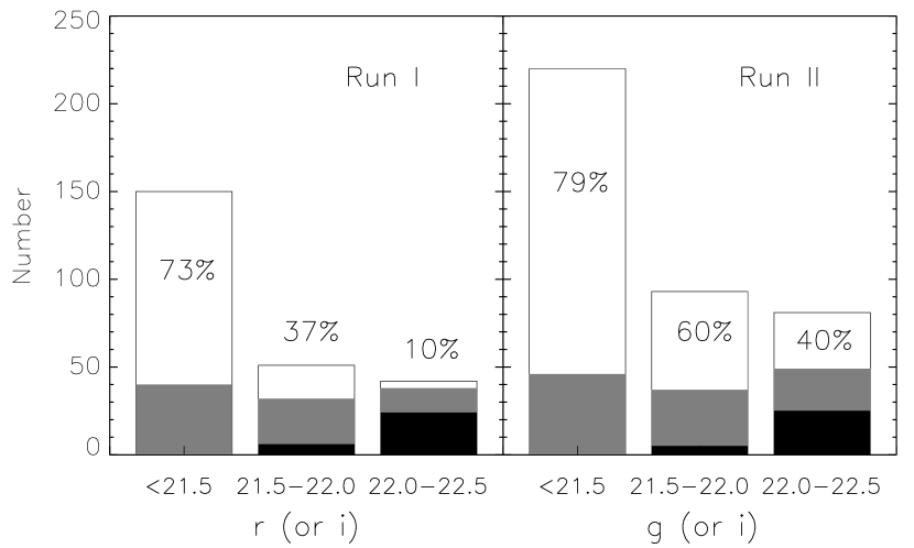
Figure 4: The numbers of candidates observed and the selection efficiencies in the two runs. The black areas are spectroscopically unidentifiable objects, the gray areas are identified as non-quasars, and the blank regions are identified as quasars. The fractions of quasars are also given within or above the bars. Note that $i$ magnitude is used for high-$z$ ($z\gtrsim 3$) candidates.

Figure 4 illustrates the numbers of candidates observed and the selection efficiencies in the two runs. In Figure 4, the black areas are unidentifiable objects, the gray areas are identified as non-quasars, and the blank regions are identified as quasars. The fractions of quasars are also given within or above the bars. The total selection efficiency in Run II is $\sim 66\%$, and the efficiency at $g<21.5$ is as high as 79%. Much of the low efficiency is produced by the mid-$z$ candidates, where the total efficiency and the efficiency at $g<21.5$ are 43% and 35%, respectively. In Run I, the selection efficiency at $r>22.0$ is only 10%. The average epoch number $N_{epoch}$ of the data in Run I is 7.4, smaller than 13.0 in Run II, so the photometric errors are relatively larger, and the quasar selection is thus less efficient. Due to the low efficiency at $r>22.0$, the quasar selection in Run I is only complete to $r=22.0$. In Run II, the quasar selection probes to $g=22.5$. Note that for a quasar with a power-law continuum slope of $-0.5$ (see $\S$ 3.3), its $g$ magnitude is fainter than $r$ magnitude by 0.15. We also improved the selection criteria in Run II based on Run I (see $\S 2.2$), so the selection efficiency in Run II was increased.

Figure 5 gives the $i$ magnitude and redshift distributions of the SFQS sample. The dashed profiles are from the SDSS DR3 (Schneider et al., 2005), and have been scaled to compare with our survey. The SFQS sample is about $2\sim 3$ magnitudes fainter than the SDSS main survey as we see in the left panel. In the right panel, our survey peaks at a similar redshift $z\sim 1.6$ to the SDSS main survey, but contains a larger fraction of $2<z<3$ quasars due to our more complete selection of quasar candidates in this redshift range. There is a small dip at $z\approx 2.7$. It may be caused by the fact that we missed bright mid-$z$ quasars in Run I.

Figure 6 shows six sample spectra obtained by our survey: (a) A typical bright quasar with $g=20.11$; (b) A typical faint quasar with $g=22.36$; (c) A typical low-$z$ quasar at $z=0.56$; (d) The most distant quasar observed in the two runs at $z\sim 5$; (e) A high-$z$ quasar with a broad CIII] emission line and a series of narrow emission lines such as Ly$\alpha$, and CIV. (Zakamska et al., 2003); (f) A broad absorption line quasar at $z=2.02$.

Table 2 presents the quasar catalog of the SFQS. Column 1 gives the name of each quasar, and column 2 is the redshift. Column 3 and 4 list the apparent magnitude $g$ and the rest-frame absolute magnitude $M_{g}$. The slope $\alpha$ of the power-law continuum for each quasar is given in column 5. Measurements of $M_{g}$ and $\alpha$ are discussed in the next subsection. The full Table 2 will appear in the electronic edition.

3.3 Determination of continuum properties

We determine the continuum properties for each quasar using the observed spectrum and the SDSS photometry. Hectospec gives spectra from $\sim$ 3700 to $\sim$ 9200 Å; however, at the faint end of the sample, the observed spectra have low signal-to-noise ratios and could be strongly effected by errors in flux calibration or sky subtraction. The accurate broadband photometry of the SDSS provides us an alternative way to determine the continuum properties from both the observed spectrum and the SDSS photometry (Fan et al., 2001b). For a given quasar, we obtain the intrinsic spectrum by fitting a model spectrum to the broadband photometry. The model spectrum is a power-law continuum plus emission lines. For the power-law continuum $f_{\nu}=A\times{\nu}^{\alpha}$, we do not assume a uniform slope $\alpha=-0.5$, instead, we determine the slope and the normalization $A$ for each quasar. To obtain model emission lines, we measure the strength of the observed emission line with the highest signal-to-noise ratio. The strengths of other emission lines are determined using the line strength ratios from the composite spectrum given by Vanden Berk et al. (2001).

The SDSS magnitudes $m^{model}$ for the model spectrum are directly calculated from the model spectrum itself. Then $\alpha$ and $A$ are determined by minimizing the differences between the model magnitudes $m^{model}$ and the SDSS photometry $m^{obs}$,

$${\chi}^{2}=\sum(\frac{m^{model}_{i}-m^{obs}_{i}}{\sigma^{obs}_{i}})^{2},$$ (3)

where $\sigma^{obs}_{i}$ is the SDSS photometry error. We fix the value of $\alpha$ in the range of $-1.1<\alpha<0.1$. In Equation 3, we only use the bands that are not dominated by Ly$\alpha$ absorption systems. With the information of intrinsic spectra and redshifts, we calculate the absolute magnitudes. The slope $\alpha$ and absolute magnitude $M_{g}$ are given in Table 2.

4 Optical luminosity function of faint quasars

In this section, we correct for the photometric, coverage, and spectroscopic incompleteness and the morphology bias. We then use the traditional $1/V_{a}$ method (Avni & Bahcall, 1980) to derive a binned estimate of the luminosity function for the SFQS sample and model the luminosity function using maximum likelihood analysis.

4.1 Completeness corrections

The photometric incompleteness arises from the color selection of quasar candidates. It is described by the selection function, the probability that a quasar with a given magnitude, redshift, and intrinsic spectral energy distribution (SED) meets the color selection criteria (e.g. Fan et al., 2001b). By assuming that the intrinsic SEDs have certain distributions, we can calculate the average selection probability as a function of magnitude and redshift. To do this, we first calculate the synthetic distribution of quasar colors for a given ($M_{g},z$), following the procedures in Fan (1999), Fan et al. (2001b) and Richards et al. (2006). Then we calculate the SDSS magnitudes from the model spectra and incorporate photometric errors into each band. For an object with given ($M_{g},z$), we generate a database of model quasars with the same ($M_{g},z$). The detection probability for this quasar is then the fraction of model quasars that meet the selection criteria.

Figure 7 gives the selection probabilities as the function of $M_{g}$ and $z$ in the two runs. The contours are selection probabilities from 0.2 to 0.8 with an interval of 0.2, and heavy lines (probability $=0.2$) illustrate the limiting magnitudes. The solid circles are the locations of sample quasars. The two selection functions are different due to the different color selection criteria used. The striking difference is the detection probabilities in the mid-$z$ range, where quasars are difficult to select by their SDSS colors. In Run I, the probabilities in the mid-$z$ range are very low for luminous quasars. But in Run II, the selection in this range is greatly improved. This makes an almost homogeneous selection from $z=0$ to $z>5$. Due to this improved selection, we are able to correct for the incompleteness down to $M_{g}=-22.0$, $-23.0$, $-24.0$ at $z<2$, $z<3$, and $z<4$, respectively.

The second incompleteness is the coverage incompleteness, which comes from the fact that we did not observe all candidates in the fields due to the limited fiber density of Hectospec. To correct this effect, we assume that the selection efficiency of unobserved candidates is the same as that of observed ones.

The third incompleteness, spectroscopic incompleteness, comes from the fact that we cannot identify some faint candidates due to their weak flux observed on Hectospec. To correct this incompleteness, we assume that unidentifiable candidates have the same selection efficiency of identified ones with the same magnitudes. From the two runs we know that, with the capacity of Hectospec and the integration time of $\sim 180$ minutes, the emission lines of a typical broad-line quasar with $g\sim 22.5$ should be visible in the Hectospec spectra, so unidentifiable candidates are either weak-line quasars, or not quasars. Therefore this correction may give an upper limit.

Another incompleteness arises from the morphology bias. The candidates we observed are point sources, but faint point sources could be mis-classified as extended sources by the SDSS photometric pipeline (e.g. Scranton et al., 2002). The best way to correct this incompleteness is to observe a sample of extended sources that satisfy our selection criteria, and find the fraction of quasars among them. The definition of star-galaxy classification in the SDSS photometric pipeline gives us an alternative way. In the SDSS photometric pipeline, an object is defined as a $galaxy$ (extended object) if $psfMag-cmodelMag>0.145$, where $psfMag$ is the PSF magnitude, and $cmodelMag$ is the composite model magnitude determined from the best-fitting linear combination of the best-fitting de Vaucouleurs and exponential model for an object’s light profile (Abazajian et al., 2004). Similar to Scranton et al. (2002), we define the difference between $psfMag$ and $cmodelMag$ as $concentration$. To correct the morphology bias, we plot the $concentration$ distribution vs. object counts as shown in Figure 8, where the dash-dotted lines separate $stars$ and $galaxies$ by definition. At $g>22.0$, the star locus and the galaxy locus begin to mix heavily, and the objects near the separation lines may be mis-classified. To estimate the real numbers of point and extended sources, we use double Gaussians to fit each component of the $star$ and $galaxy$ loci as shown in the figure. Then the fraction of point sources misclassified as extended ones are obtained from the best fits. They are 10% for $22.0<g<22.2$, 24% for $22.2<g<22.4$, and 31% for $22.4<g<22.5$.

In Run I and Run II we only select point sources. Although we have corrected the morphology bias, our sample could still be biased by not including objects in which the host galaxies are apparent. So the low-$z$ QLF at the faint end may be affected by quasar host galaxies. We plan to observe a sample of extended sources, and correct the morphology bias and the effect of host galaxies in the next observing run.

4.2 1/$V_{a}$ estimate and maximum likelihood analysis

We derive a binned estimate of the luminosity function for the SFQS sample using the traditional $1/V_{a}$ method (Avni & Bahcall, 1980). The available volume for a quasar with absolute magnitude $M$ and redshift $z$ in a magnitude bin $\Delta M$ and a redshift bin $\Delta z$ is

$$V_{a}=\int_{\Delta M}\int_{\Delta z}p(M,z)\frac{dV}{dz}dzdM,$$ (4)

where $p(M,z)$ is a function of magnitude and redshift and used to correct sample incompleteness. Then the luminosity function and the statistical uncertainty can be written as

$$\Phi(M,z)=\sum\frac{1}{V_{a}^{i}},\ \ \sigma(\Phi)=\left[\sum(\frac{1}{V_{a}^{i}})^{2}\right]^{1/2},$$ (5)

where the sum is over all quasars in the bin. This is essentially the same as the revised $1/V_{a}$ method of Page & Carrera (2000), since $p(M,z)$ has already corrected the incompleteness at the flux limits.

The QLF derived from the $1/V_{a}$ estimate is shown in Figure 9, which gives the QLF from $z=0.5$ to 3.6, with a redshift interval of $\Delta z\approx 0.5$. In each redshift bin, the magnitude bins are chosen to have exactly the same numbers of quasars except the brightest one. Solid symbols represent the QLF corrected for all four incompletenesses in $\S 4.1$, and open symbols represent the QLF corrected for all incompletenesses except the spectroscopic incompleteness. Our sample contains two subsamples from Run I and Run II. The two subsamples are weighted by their available volumes in each magnitude-redshift bin when combined. In Run I, the selection efficiency at $r>22.0$ is only 10%, so we do not include the quasars of $r>22.0$ in the 1/$V_{a}$ estimate. We also exclude the Run I quasars in the brightest bins at $2.0<z<3.0$, due to the low selection completeness in this range.

Our sample contains a small fraction of luminous quasars. By comparing the SFQS QLF with the results of the 2QZ, 2SLAQ, and SDSS (see Figure 11 and Figure 12 in $\S 5.3$), one can see that the QLF has steep slopes at the bright end (from the 2QZ, 2SLAQ, or SDSS) and much flatter slopes at the faint end (from the SFQS), clearly showing a break in the QLF, thus we will use the double power-law form to model the QLF. At $z>2.0$, quasars show strong density evolution. A double power-law QLF with density evolution requires at least six parameters, however, this sample is not large enough to determine so many parameters simultaneously. Therefore we break the sample to two subsamples, $0.5<z<2.0$ and $2.0<z<3.6$, and use fewer free parameters to model them separately, based on reasonable assumptions. We will model the low-$z$ and high-$z$ quasars simultaneously when we obtain more than 1000 quasars in the future.

4.2.1 QLF at 0.5 $<z<$ 2.0

As the first step, we try a single power-law form $\Phi(L)\propto L^{\beta}$ to model the observed QLF. The slope $\beta$ determined from the best fit is $-1.40$, much flatter than the bright-end slopes ($-3.0\sim-3.5$) of the QLFs from the 2QZ (Boyle et al., 2000; Croom et al., 2004), SDSS (Richards et al., 2006), and 2SLAQ (Richards et al., 2005). This confirms the existence of the break in the slope. We also use the single power-law form to model the three individual redshift bins. The best fit slopes at $0.5<z<1.0$, $1.0<z<1.5$, and $1.5<z<2.0$ are $-1.45_{-0.3}^{+0.2}$, $-1.40_{-0.2}^{+0.1}$, and $-1.35_{-0.2}^{+0.1}$, respectively. They are consistent within $1\sigma$ level, so there is no strong evolution in the slope at the faint end.

To characterize the QLF at $0.5<z<2.0$, we use the double power-law form with PLE, which expressed in magnitudes is,

$$\Phi_{L}(M_{g},z)=\frac{\Phi(M_{g}^{\ast})}{10^{0.4(\alpha+1)(M_{g}-M_{g}^{\ast}(z))}+10^{0.4(\beta+1)(M_{g}-M_{g}^{\ast}(z))}}.$$ (6)

In the case of PLE models, the evolution of the characteristic magnitude $M_{g}^{\ast}(z)$ can be modeled as different forms, such as a second-order polynomial evolution $M_{g}^{\ast}(z)=M_{g}^{\ast}(0)-2.5(k_{1}z+k_{2}z^{2})$, an exponential form $M_{g}^{\ast}(z)=M_{g}^{\ast}(0)-1.08k\tau$, where $\tau$ is the look-back time, or, a form of $M_{g}^{\ast}(z)=M_{g}^{\ast}(0)-2.5k(1+z)$ (e.g. Boyle et al., 2000; Croom et al., 2004). Croom et al. (2004) has shown that low-$z$ QLF can be well fit by both second-order polynomial or exponential evolution in the $\Lambda$ cosmology. In this paper the quasar sample is still small, so we do not fit all models and justify their validity; instead, we take the exponential form, which uses fewer parameters.

We use maximum likelihood analysis to find the best fits. The likelihood function (e.g. Marshall et al., 1983; Fan et al., 2001b) can be written as

$$S=-2\sum ln[\Phi(M_{i},z_{i})p(M_{i},z_{i})]+2\int\int\Phi(M,z)p(M,z)\frac{dV}{dz}dzdM,$$ (7)

where the sum is over all quasars in the sample. Our sample does not contain enough bright objects, which makes it difficult to determine the slope at the bright end. We thus fix the bright-end slope to the value of $\alpha=-3.25$ given by Croom et al. (2004). The best fits are, $\alpha=-3.25$ (fixed), $\beta=-1.25_{-0.15}^{+0.10}$, $k=7.50_{-0.35}^{+0.40}$, $M_{g}^{\ast}(0)=-19.50_{-0.35}^{+0.40}$, and $\Phi(M_{g}^{\ast})=1.84\times 10^{-6}$ Mpc^-3 mag^-1. The $\chi^{2}$ of this fit is 15.0 for 15 degrees of freedom by comparing the $1/V_{a}$ estimate and the model prediction. The solid lines in Figure 9 are the best model fits. For comparison, the dashed lines are the best fit at $1.5<z<2.0$. One can see that the density of quasars increases from $z$ = 0.5 to 2.0, then decreases at higher redshift.

As stated in $\S$ 4.1, the correction of the spectroscopic incompleteness may only provide an upper limit. In Figure 9, solid symbols represent the QLF corrected for all four incompleteness in $\S 4.1$, and open symbols represent the QLF corrected for all incompleteness except the spectroscopic incompleteness. One can see that the spectroscopic incompleteness only affects the faintest bins. The best model fit shows that, without the correction for the spectroscopic incompleteness, the slope at $0.5<z<2.0$ flattens from $-1.25_{-0.15}^{+0.10}$ to $-1.10_{-0.15}^{+0.10}$. The variation in the slope is within $1\sigma$ level.

4.2.2 QLF at 2.0 $<z<$ 3.6

At $z>2.0$, the QLF cannot be modeled by PLE, and density evolution is needed. We add a density evolution term $\rho_{D}(z)$ into the double power-law form to model the QLF at $z>2.0$. The double power-law model with density evolution expressed in magnitudes is,

$$\Phi_{H}(M_{g},z)=\frac{\Phi(M_{g}^{\ast})\rho_{D}(z)}{10^{0.4(\alpha+1)(M_{g}-M_{g}^{\ast}(z))}+10^{0.4(\beta+1)(M_{g}-M_{g}^{\ast}(z))}},$$ (8)

where we take the exponential form for the evolution of characteristic magnitude $M_{g}^{\ast}(z)$ as we do for $z<2$, and take an exponential form of $\rho_{D}(z)=10^{-B(z-2)}$ for the density evolution at a given magnitude (e.g. Schmidt, Schneider, & Gunn, 1995; Fan et al., 2001b). The single power-law model with density evolution shows that the QLF at $2.0<z<3.6$ has a slope of $-1.70$, flatter than the bright-end slopes ($-2.5\sim-3.5$) from the COMBO-17 (Wolf et al., 2003), SDSS (Richards et al., 2006) and Fan et al. (2001b). This indicates the existence of the break in the QLF at $2.0<z<3.6$.

We use the double power-law form with density evolution to model the observed QLF at $2.0<z<3.6$. As we do for $z<2.0$, we fix the bright-end slope $\alpha$ as $-3.25$. The parameters $k$ and $M_{g}^{\ast}(0)$ are also fixed to the values determined from $0.5<z<2.0$. There are three parameters $\beta$, $B$, and $\Phi(M_{g}^{\ast})$ that we need to derive. $\Phi(M_{g}^{\ast})$ is not a free parameter, because Equations 6 and 8 must be consistent at $z=2$. Figure 9 shows that, at $M_{g}\sim-23$, the density at $1.5<z<2.0$ and the density at $2.0<z<2.5$ are roughly the same. So we connect Equations 6 and 8 through $\Phi_{L}(M_{g}=-23,z=2)=\Phi_{H}(M_{g}=-23,z=2)$. Then $\Phi(M_{g}^{\ast})$ can be derived from $\beta$ and $B$ by this relation. We use maximum likelihood analysis to determine the two free parameters $\beta$ and $B$ as well as $\Phi(M_{g}^{\ast})$. The best fits are, $\beta=-1.55\pm 0.20$, $B=0.45\pm 0.15$, and $\Phi(M_{g}^{\ast})=1.02\times 10^{-6}$ Mpc^-3 mag^-1. The $\chi^{2}$ of this fit is 10.4 for 11 degrees of freedom. The solid lines in Figure 9 are the best model fits.

Our sample contains only 5 quasars at $z>3.6$, which is lower than what we expected if the power-law slope of the QLF at $3.6<z<5.0$ is $\sim-2.4\pm 0.2$ (Richards et al., 2006). This result implies that the faint-end slope of the QLF at $3.6<z<5.0$ is also flatter than that at the bright end.

5 Discussion

5.1 Luminosity-dependent density evolution

It is convenient to show the quasar evolution by plotting the space density as a function of redshift. Our sample spans a large redshift range, covering the mid-$z$ range with good completeness. Figure 10 gives the integrated comoving density as the function of $z$ for three magnitude ranges, $M_{g}<-22.5$, $-23.5$, and $-24.5$, respectively. We use the redshift bins from $z=0.4$ to 3.6 with an interval of $\Delta z=0.4$. For the bins at $2.2<z<3.0$, we exclude quasars with $M_{g}<-24.5$ in Run I, due to the low selection completeness in this range. We also exclude incomplete bins in Figure 10. At low redshift, the space density steadily increases from $z\sim 0.5$ to $\sim 2$. Then it decreases toward high redshift. The quasar evolution peaks at $z\sim 2$ in the range of $M_{g}<-22.5$. Solid curves are integrated densities calculated from the best model fits in $\S$ 4.2, while dotted, dashed and dot-dashed curves represent the integrated densities from the SDSS (Richards et al., 2006), 2QZ (Boyle et al., 2000), and Schmidt, Schneider, & Gunn (1995, SSG), respectively. X-ray surveys indicate that X-ray selected quasars and AGNs exhibit so-called “cosmic downsizing”: luminous quasars peak at an earlier epoch in the cosmic history than fainter AGNs (e.g. Ueda et al., 2003; Barger et al., 2005; Hasinger, Miyaji, & Schmidt, 2005). We cannot see the cosmic downsizing from the SFQS sample due to the small dynamical range in magnitude and large errors bars. However, the peak of $z\sim 2$ for the SFQS sample is later in cosmic time than the peak of $z\sim 2.5$ found from luminous quasar samples, such as the SDSS (Richards et al., 2006).

5.2 Comparison to other surveys

In this section we compare the SFQS QLF with QLFs derived from the 2QZ (Boyle et al., 2000), SDSS (Richards et al., 2006), 2SLAQ (Richards et al., 2005), COMBO-17 (Wolf et al., 2003), and CDF (Barger et al., 2005). The survey areas and magnitude limits are sketched in Figure 2. Because different surveys use different cosmological models, we convert their QLFs to the QLFs expressed in the cosmological model that we use. First, absolute magnitude $M^{\prime}$ is converted to $M$ by $M^{\prime}-M=-5log_{10}\frac{d_{L}^{{}^{\prime}}}{d_{L}}$, where $d_{L}^{{}^{\prime}}$ and $d_{L}$ are luminosity distances in different cosmologies. Then magnitudes in different wavebands are converted to $M_{g}$ in the same cosmology by $M_{g}=M_{\lambda}+2.5\alpha log_{10}\frac{\lambda_{g}}{\lambda}$, where $\alpha$ is the slope of the power-law continuum, and we assume $\alpha=-0.5$; $\lambda_{g}$ and $\lambda$ are the effective wavelengths of the two different wavebands. Finally spatial density $\rho^{{}^{\prime}}$ in a $M$-$z$ bin is converted to $\rho$ by $\rho=\rho^{{}^{\prime}}\frac{V_{a}^{{}^{\prime}}}{V_{a}}$, where $V_{a}$ and $V_{a}^{{}^{\prime}}$ are available comoving volumes in the different cosmologies.

Figure 11 gives the comparison with the 2QZ (Boyle et al., 2000) and 2SLAQ (Richards et al., 2005) at $0.5<z<2.0$. Compared to the 2QZ and 2SLAQ, the SFQS probes to higher redshifts and fainter magnitudes. Solid circles and open triangles in Figure 11 are the SFQS QLF and 2SLAQ QLF, respectively. The dotted and dashed lines represent the 2QZ QLF, which is an average QLF calculated using $<\Phi(M,z)>=\frac{\int_{\Delta z}\Phi(M,z)dV}{\int_{\Delta z}dV}$, where $\Phi(M,z)$ is the best-fitting double power-law model with a second-order polynomial luminosity evolution from Boyle et al. (2000). The dashed-line parts are roughly the range that the observed 2QZ QLF really covered (Boyle et al., 2000). The solid lines are the best model fits of the SFQS QLF. They give a good fit to all three QLFs. At the bright end of the QLF, the SFQS, 2QZ, and 2SLAQ agree well. At the faint end, the 2QZ predicts a higher density and a steeper slope than the SFQS. By combining the deep SFQS with the 2QZ and 2SLAQ, one can see that there is clearly a break in the QLF slope.

Figure 12 shows the comparison with the SDSS (Richards et al., 2006) and COMBO-17 (Wolf et al., 2003) at $0.5<z<3.6$. The SDSS is a shallow survey covering a large redshift range. The COMBO-17 survey uses photometric redshifts, and collects quasars in an area of $\lesssim$1 deg². In Figure 12, solid circles and open triangles are the SFQS QLF and SDSS QLF, respectively. The dashed lines represent the COMBO-17 QLF, which is an average QLF calculated from the best model fitting of Wolf et al. (2003) using the same method that we did above. The solid lines are the best model fits of the SFQS QLF, and they give a reasonable fit to both SDSS and SFQS QLFs. The SFQS is more than 2 magnitudes deeper than the SDSS, but their QLFs are consistent at all redshifts. The combination of the two QLFs also shows the existence of a break in the slope. At $1.0<z<3.6$, the COMBO-17 QLF agrees well with the SFQS QLF, although it has a flatter slope than the SDSS at the bright end.

Figure 13 shows the comparison with the CDF survey of quasars and AGNs (Barger et al., 2005). Barger et al. (2005) determine the luminosity functions for both type I and type II AGNs selected from hard X-ray surveys, and find a downturn at the faint end of type I AGN luminosity function. We convert absolute magnitudes and X-ray luminosities to bolometric luminosities using the method given by Barger et al. (2005), and compare the SFQS QLF (solid circles) with the type I AGN hard X-ray luminosity function (open triangles and squares) of Barger et al. (2005) in Figure 13. At the bright end of the QLF, the two surveys are consistent at all redshifts. At the faint end, they agree well at $1.5<z<2.0$, however, at $0.5<z<1.5$, Barger et al. (2005) has significantly higher ($\sim 2\sigma$) densities. One can also see that the SFQS does not probe faint enough to reach the turndown seen by Barger et al. (2005).

6 Summary

This paper presents the preliminary results of a deep spectroscopic survey of faint quasars selected from the SDSS Southern Survey, a deep imaging survey, created by repeatedly scanning a 270 deg² area. Quasar candidates are selected from the co-added catalog of the deep data. With an average epoch number $N_{epoch}\sim 13$, the co-added catalog enables us to select much fainter quasars than the quasar spectroscopic sample in the SDSS main survey. We modify SDSS color selection to select quasar candidates, so that they cover a large redshift range at $z<5$, including the range of $2<z<3$ with good completeness. Follow-up spectroscopic observations were carried out on MMT/Hectospec in two observing runs. With the capacity of Hectospec, the selection efficiency of faint quasars in Run II is $\sim$80% at $g<21.5$, and acceptable at $g>21.5$ (60% for $21.5<g<22.0$ and 40% for $22.0<g<22.5$). The preliminary sample of the SFQS contains 414 quasars and reaches $g=22.5$.

We use the $1/V_{a}$ method to derive a binned estimate of the QLF. By combining the SFQS QLF with the QLFs of the 2QZ, 2SLAQ, and SDSS, we conclude that there is a break in the QLF. We use the double power-law form with PLE to model the observed QLF at $0.5<z<2.0$, and the double power-law form with an exponential density evolution to model the QLF at $2.0<z<3.6$. The QLF slopes at the faint end ($-1.25$ at $0.5<z<2.0$ and $-1.55$ at $2.0<z<3.6$) are much flatter than the slopes at the bright end, indicating the existence of the break at all redshifts probed. The luminosity-dependent density evolution model shows that the quasar evolution at $M_{g}<-23.5$ peaks at $z\sim 2$, which is later in the cosmic time than the peak of $z\sim 2.5$ found from luminous quasar samples.

Our survey is compared to the 2QZ (Boyle et al., 2000), SDSS (Richards et al., 2006), 2SLAQ (Richards et al., 2005), COMBO-17 (Wolf et al., 2003), and CDF (Barger et al., 2005). The SFQS QLF is consistent with the results of the 2QZ, SDSS, 2SLAQ and COMBO-17. The SFQS QLF at the faint end has a significantly lower density at $0.5<z<1.5$ than does the CDF. The preliminary sample of the SFQS is still small, and statistical errors are large. We plan to obtain more faint quasars from future observations and establish a complete quasar sample with more than 1000 quasars over an area of 10 deg².

Figure 1: $u-g$, $g-r$ color-color diagrams for point sources ($20.5<g<21.0$) in the SDSS main survey and deep survey with $N_{epoch}\sim 13$. Each panel includes 10,000 objects. Compared to the main survey, the stellar locus in the deep survey is more concentrated, and $UVX$ quasar candidates (confined by solid lines) are well separated from the stellar locus.

Figure 2: The comparison between the SFQS and the LBQS (Foltz et al., 1987), 2QZ (Boyle et al., 2000; Croom et al., 2004), SDSS (Richards et al., 2002), 2SLAQ (Richards et al., 2005), COMBO-17 (Wolf et al., 2003) and CDF (Barger et al., 2005, the area given here is the total area of CDF-N and CDF-S) surveys of quasars and AGNs.

Figure 3: The selection of $UVX$ and mid-$z$ candidates from $g=16.0$ to 22.5 in $u-g$, $g-r$ diagrams. The inner parts of the diagrams are shown in contours, which linearly increase inwards in the density of stars. For the purpose of comparison, each panel includes 20,000 objects. The regions confined by solid lines are our selection of $UVX$ and mid-$z$ candidates.

Figure 5: The $i$ magnitude and redshift distributions of the SFQS sample compared with the SDSS main survey. The dashed profiles are from the SDSS DR3 (Schneider et al., 2005), and have been scaled to compare with our survey.

Figure 6: Six sample spectra obtained by MMT/Hectospec. The spectra are binned by 11 pixels. The redshift of each quasar is also given in the figure.

Figure 7: Selection function of faint quasars as a function of $M_{g}$ and $z$. The contours are selection probabilities from 0.2 to 0.8 with an interval of 0.2. The solid circles are the locations of quasars in our sample. Heavy lines (probability $=0.2$) illustrate the limiting magnitudes.

Figure 8: Correction for the morphology bias. The vertical dot-dashed lines separate $stars$ and $galaxies$ by the definition of the SDSS photometric pipeline. Dotted and dashed lines are the best fits of the double Gaussian components of $stars$ and $galaxies$, respectively. Solid lines are the sum of all components.

Figure 9: QLF derived from the traditional $1/V_{a}$ method. Solid circles represent the QLF corrected for all four incompletenesses in $\S$ 4.1, while open circles represent the QLF corrected for all incompletenesses except the spectroscopic incompleteness. Solid lines are the best model fits from $\S$ 4.2. For comparison, the dashed line is the best model fit of the QLF at $1.5<z<2.0$.

Figure 10: Integrated comoving density as a function of $z$ for three magnitude ranges, $M_{g}<-22.5$, $-23.5$, and $-24.5$, respectively. The redshift bins are from $z=0.4$ to 3.6 with the interval of $\Delta z=0.4$. We do not include incomplete bins. Solid curves are integrated densities calculated from the best model fits in $\S$ 4.2, while dotted, dashed and dot-dashed curves are the integrated densities from the SDSS (Richards et al., 2006), 2QZ (Boyle et al., 2000), and SSG (Schmidt, Schneider, & Gunn, 1995), respectively.

Figure 11: Comparison with the 2QZ (Boyle et al., 2000) and 2SLAQ (Richards et al., 2005). Solid circles and open triangles are the SFQS QLF and 2SLAQ QLF, respectively. The dotted and dashed lines represent the 2QZ QLF, calculated from the best model fits of Boyle et al. (2000). The dashed-line parts are roughly the range of luminosity that the observed 2QZ QLF actually covered (Boyle et al., 2000). The solid lines are the best model fits of the SFQS QLF.

Figure 12: Comparison with the SDSS (Richards et al., 2006) and COMBO-17 (Wolf et al., 2003). Solid circles and open triangles are the SFQS QLF and SDSS QLF, respectively. The dashed lines represent the COMBO-17 QLF, calculated from the best model fits of Wolf et al. (2003). The solid lines are the best model fits of the SFQS QLF.

Figure 13: Comparison with the CDF survey (Barger et al., 2005). Solid circles represent the SFQS QLF. Open triangles and squares are from Figure 22 of Barger et al. (2005).

Table 1: Central positions and exposure time for the 5 Hectospec fields

	Date	RA(J2000)	Dec(J2000)	$t_{exp}$(min)
Run I	Jun 13	$21^{h}34^{m}00{\fs}0$	$00{\arcdeg}06{\arcmin}00{\farcs}0$	100
	Jun 15	$21^{h}34^{m}00{\fs}0$	$00{\arcdeg}06{\arcmin}00{\farcs}0$	100
	Jun 20	$21^{h}30^{m}00{\fs}0$	$00{\arcdeg}06{\arcmin}00{\farcs}0$	100
Run II	Nov 09	$23^{h}16^{m}00{\fs}0$	$-00{\arcdeg}06{\arcmin}00{\farcs}0$	120
	Nov 11	$23^{h}40^{m}00{\fs}0$	$-00{\arcdeg}06{\arcmin}00{\farcs}0$	180
	Nov 13	$02^{h}04^{m}00{\fs}0$	$-00{\arcdeg}06{\arcmin}00{\farcs}0$	80
	Nov 19	$02^{h}04^{m}00{\fs}0$	$-00{\arcdeg}06{\arcmin}00{\farcs}0$	120

Table 2: Quasar sample for the SFQS survey

Name (J2000 Coordinates)	Redshift	$g$	$M_{g}$	$\alpha$
SDSS J231601.68$-$001237.0	2.00	21.69	-23.08	-0.23
SDSS J231548.40$-$003022.7	1.53	20.73	-23.60	-0.44
SDSS J231527.54$-$001353.8	1.33	20.97	-23.26	-0.54
SDSS J231541.51$-$003137.2	1.72	21.73	-22.61	-0.31
SDSS J231422.26$+$000315.7	3.22	21.38	-24.05	0.10
SDSS J231442.27$-$000937.2	3.30	21.09	-25.26	-0.49
SDSS J231534.22$-$002610.0	0.58	21.29	-21.02	-1.07
SDSS J231519.33$-$001129.5	3.06	22.17	-24.47	-1.10
SDSS J231504.04$-$001434.2	2.10	22.17	-23.05	-0.41
SDSS J231446.30$-$002206.9	2.97	21.97	-24.12	-0.69
$\cdot\cdot\cdot$

References

- Abazajian et al. (2004) Abazajian, K., et al. 2004, AJ, 128, 502
- Avni & Bahcall (1980) Avni, Y., & Bahcall, J. N. 1980, ApJ, 235, 694
- Barger et al. (2005) Barger, A. J., Cowie, L. L., Mushotzky, R. F., Yang, Y., Wang, W. H., Steffen, A. T., & Capak, P. 2005, AJ, 129, 578
- Blanton et al. (2003) Blanton, M. R., Lin, H., Lupton, R. H., Maley, F. M., Young, N., Zehavi, I., & Loveday, J. 2003, AJ, 125, 2276
- Blanton et al. (2005) Blanton, M. R., et al. 2005, AJ, 129, 2562
- Boyle, Shanks, & Peterson (1988) Boyle, B. J., Shanks, T., & Peterson, B. A. 1988, MNRAS, 235, 935
- Boyle & Terlevich (1998) Boyle, B. J., & Terlevich, R. J. 1998, MNRAS, 293, L49
- Boyle et al. (2000) Boyle, B. J., Shanks, T., Croom, S. M., Smith, R. J., Miller, L., Loaring, N., & Heymans, C. 2000, MNRAS, 317, 1014
- Brown et al. (2006) Brown, M. J. I., et al. 2006, ApJ, 638, 88
- Cool et al. (2006) Cool, R., et al. 2006, in preparation
- Croom et al. (2004) Croom, S. M., Smith, R. J., Boyle, B. J., Shanks, T., Miller, Outram, P. J., & L., Loaring, N. 2004, MNRAS, 317, 1014
- Croton et al. (2006) Croton, D. J., et al. 2006, MNRAS, 365, 11
- Eisenstein et al. (2001) Eisenstein, D. J., et al. 2001, AJ, 122, 2267
- Fabricant et al. (1998) Fabricant, D. G., Hertz, E. N., Szentgyorgyi, A. H., Fata, R. G., Roll, J. B., & Zajac, J. M. 1998, Proc. SPIE, 3355, 285
- Fan (1999) Fan, X. 1999, AJ, 117, 2528
- Fan et al. (1999) Fan, X., et al. 1999, AJ, 118, 1
- Fan et al. (2000) Fan, X., et al. 2000, AJ, 119, 1
- Fan et al. (2001a) Fan, X., et al. 2001a, AJ, 121, 31
- Fan et al. (2001b) Fan, X., et al. 2001b, AJ, 121, 54
- Foltz et al. (1987) Foltz, C. B., Chaffee, F. H., Hewett, P. C., MacAlpine, G. M., Turnshek, D. A., Weymann, R. J., & Anderson, S. F. 1987, AJ, 94, 1423
- Fukugita et al. (1996) Fukugita, M., Ichikawa, T., Gunn, J. E., Doi, M., Shimasaku, K., & Schneider, D. P. 1996, AJ, 111,1748
- Goldschmidt & Miller (1998) Goldschmidt, P., & Miller, L. 1998, MNRAS, 293, 107
- Gray et al. (2004) Gray, A. G., Moore, A. W., Nichol, R. C., Connolly, A. J., Genovese, C., & Wasserman, L. 2004, ASPC, 314, 249
- Gunn et al. (1998) Gunn, J. E., et al. 1998, AJ, 116, 3040
- Gunn et al. (2006) Gunn, J. E., et al. 2006, AJ, submitted
- Hawkins & Véron (1995) Hawkins, M. R. S., & Véron, P. 1995, MNRAS, 275, 1102
- Hasinger, Miyaji, & Schmidt (2005) Hasinger, G., Miyaji, T., & Schmidt, M. 2005, A&A, 441, 417
- Hewett, Foltz, & Chaffee (1993) Hewett, P. C., Foltz, C. B., & Chaffee, F. H. 1993, ApJ, 406, L43
- Hogg et al. (2001) Hogg, D. W., Finkbeiner, D. P., Schlegel, D. J., & Gunn, J. E. 2001, AJ, 122, 2129
- Hopkins et al. (2005) Hopkins, P. F., Hernquist, L., Cox, T. J., Matteo, T. D., Martini, P., Robertson, B., & Springel, V. 2005, ApJ, 630, 705
- Ivezić et al. (2004) Ivezić, Ž., et al. 2004, Astonomische Nachrichten, 325, 583
- Kauffmann & Haehnelt (2000) Kauffmann, G., & Haehnelt, M. 2000, MNRAS, 311, 576
- Kennefick, Djorgovski, & De Carvalho (1995) Kennefick, J. D., Djorgovski, S. G., & De Carvalho, R. R. 1995, AJ, 110, 2553
- Koo & Kron (1988) Koo, D. C., & Kron, R. G. 1988, ApJ, 325, 92
- Kurucz (1993) Kurucz, R. 1993, ATLAS9 Stellar Atmosphere Programs and 2 km/s grid. Kurucz CD-ROM No. 13. Cambridge, Mass.: Smithsonian Astrophysical Observatory, 1993, 13
- La Franca & Cristiani (1997) La Franca, F. & Cristiani, S. 1997, AJ, 113, 1517
- Lupton, Gunn & Szalay (1999) Lupton, R. H., Gunn, J. E., & Szalay, A. S. 1999, AJ, 118, 1406
- Lupton et al. (2001) Lupton, R. H., Gunn, J. E., Ivezić, Ž., Knapp, G. R., Kent, S., & Yasuda, N. 2001, in Astronomical Data Analysis Software and Systems X, edited by F. R. Harnden Jr., F. A. Primini, and H. E. Payne, ASP Conference Proceedings, 238, 269
- Marshall et al. (1983) Marshall, H. L., Avni, Y., Tananbaum, H., & Zamorani, G. 1983, ApJ, 269, 35
- Marshall et al. (1984) Marshall, H. L., Avni, Y., Braccesi, A., Huchra, J. P., Tananbaum, H., Zamorani, G. & Zitelli, V. 1984, ApJ, 283, 50
- Marshall (1985) Marshall, H. L. 1985, ApJ, 299, 109
- Martini & Weinberg (2001) Martini, P., & Weinberg, D. H. 2001, ApJ, 547, 12
- Mushotzky et al. (2000) Mushotzky, R. F., Cowie, L. L., Barger, A. J., & Arnaud, K. A. 2000, Nature, 404, 459
- Newberg & Yanny (1997) Newberg, H. J., & Yanny, B. 1997, ApJS, 113, 89
- O’Donnell (1994) O’Donnell, J. E. 1994, ApJ, 422, 158
- Page & Carrera (2000) Page, M. J., & Carrera, F. J. 2000, MNRAS, 311, 433
- Pei (1995) Pei, Y. C. 1995, ApJ, 438, 623
- Pier et al. (2003) Pier, J. R., Munn, J. A., Hindsley, R. B., Hennessy, G. S., Kent, S. M., Lupton, R. H., & Ivezic, Z. 2003, AJ, 125, 1559
- Richards et al. (2002) Richards, G. T., et al. 2002, AJ, 123, 2945
- Richards et al. (2004) Richards, G. T., et al. 2004, ApJS, 155, 257
- Richards et al. (2005) Richards, G. T., et al. 2005, MNRAS, 360, 839
- Richards et al. (2006) Richards, G. T., et al. 2006, AJ, in press (astro-ph/0601434)
- Schlegel, Finkbeiner, & Davis (1998) Schlegel, D. J., Finkbeiner, D. P., & Davis, M. 1998, ApJ, 500, 525
- Schlegel et al. (2006) Schlegel, D., et al. 2006, in preparation
- Schmidt, Schneider, & Gunn (1995) Schmidt, M., Schneider, D. P., & Gunn, J. E. 1995, AJ, 110, 68
- Schneider et al. (2005) Schneider, D. P., et al. 2005, AJ, 130, 367
- Scranton et al. (2002) Scranton, R., et al. 2002, ApJ, 579, 48
- Silverman (1986) Silverman, B. W. 1986, Density Estimation for Statistics and Data Analysis, Monographs on Statistics and Applied Probability, Vol. 26 (London: Chapman & Hall)
- Smith et al. (2002) Smith, J. A., et al. 2002, AJ, 123, 2121
- Spergel et al. (2003) Spergel, D. N., et al. 2003, ApJS, 148, 175
- Stoughton et al. (2002) Stoughton, C., et al. 2002, AJ, 123, 485
- Strauss et al. (2002) Strauss, M. A. et al. 2002, AJ, 124, 1810
- Szentgyorgyi et al. (1998) Szentgyorgyi, A. H., Cheimets, P., Eng, R., Fabricant, D. G., Geary, J. C., Hartmann, L., Pieri, M. R., & Roll, J. B. 1998, Proc. SPIE, 3355, 242
- Tucker et al. (2006) Tucker, D., et al. 2006, AJ, submitted
- Ueda et al. (2003) Ueda, Y., Akiyama, M., Ohta, K., & Miyaji, T. 2003, ApJ, 598, 886
- van Dokkum (2001) van Dokkum, P. G. 2001, PASP, 113, 1420
- Vanden Berk et al. (2001) Vanden Berk, D. E., et al. 2001, AJ, 122, 549
- Warren, Hewett, & Osmer (1994) Warren, S. J., Hewett, P. C., & Osmer, P. S. 1994, ApJ, 421, 412
- Wisotzki (2000) Wisotzki, L. 2000, A&A, 353, 853
- Wolf et al. (2003) Wolf, C., Wisotzki, L., Borch, A., Dye, S. Kleinheinrich, M., & Meisenheimer, K. 2003, A&A, 408, 499
- Worsley et al. (2005) Worsley, M. A., et al. 2005, MNRAS, 357, 1281
- Wyithe & Loeb (2003) Wyithe, J. S. B., & Loeb, A. 2003, ApJ, 595, 614
- York et al. (2000) York, D. G., et al. 2000, AJ, 120, 1579
- Zakamska et al. (2003) Zakamska, N. L., et al. 2003, AJ, 2125, 2144