Magnetohydrodynamic Shocks in Non-Equatorial Plasma Flows around a Black Hole

Abstract

We study magnetohydrodynamic (MHD) standing shocks in inflowing plasmas in a black hole magnetosphere. Fast and intermediate shock formation is explored in Schwarzschild and Kerr geometry to illustrate general relativistic effects. We find that non-equatorial standing MHD shocks are physically possible, creating a very hot plasma region close to the event horizon. Shocked downstream plasmas can be heated or magnetized depending on the values of various magnetic field-aligned parameters. Then we may expect high-energy thermal/nonthermal emissions from the shocked region. We present the properties of non-equatorial MHD shocks and discuss the shocked plasma region in the black hole magnetosphere. We also investigate the effects of the poloidal magnetic field and the black hole spin on the properties of shocks, and show that both effects can modify the distribution of the shock front and shock strength. We find for strong MHD shock formation that fast rotating magnetic fields are necessary. The physics of non-equatorial MHD shocks in the black hole magnetosphere could be very important when we are to construct the central engine model of various astrophysical phenomena.

1 Introduction

We consider a theoretical implication of a possible link between the conditions of magnetohydrodynamic (MHD) shocks and the resulting shocked hot and/or strongly magnetized plasma region very close to the black hole event horizon. In a series of our previous investigations in the context of general relativity (see, Takahashi et al. 2002, hereafter TRFT02; Rilett 2003, hereafter R03; Fukumura 2005; Takahashi et al. 2006, hereafter Paper I), it has been shown that shock formation in MHD plasmas inflowing onto a black hole can be a physically plausible mechanism for creating very hot (i.e., $T_{i}\gtrsim 10^{12}$ K for ions and $T_{e}\gtrsim 10^{9}$ K for electrons) or strongly magnetized plasma regions, which possibly could be associated with subsequent thermal/nonthermal high energy emission. These previous studies are the extension of the earlier works on hydrodynamical (HD) shock formation in black hole accretion flows (e.g., Chakrabarti 1990; Lu et al. 1997; Lu & Yuan 1998; Fukumura & Tsuruta 2004, hereafter FT04). These authors point out that black hole rotation is also important for determining the shock strength. The slow magnetosonic shock formation in relativistic ingoing flows near a black hole was first explored by TRFT02. By extending the work on shock formation in relativistic winds by Appl & Camenzind (1988), these authors solved general relativistic jump conditions in accreting plasmas. It was suggested that relativistic slow/fast MHD shocks can significantly heat up the postshock plasma (generation of hot regions), which may produce a sufficient amount of high energy radiation. R03 systematically examined the types of the preshock plasma mainly for slow MHD shocks. Fast MHD shock formation in inflowing plasmas was first studied in Paper I where a non-rotating black hole was primarily considered.

These studies were conducted mainly for the equatorial accretion flows. Therefore, a natural next step is to extend these studies to two dimensional, non-equatorial flows. Also, non-equatorial shock-heated region would be attractive as a possible high energy radiation source above an accretion disk in the central engine of active galactic nuclei (AGNs). Therefore, we investigate in this paper the polar angle dependence of various shock properties (e.g., shock radius, compression ratio, number density, magnetization, entropy generation and so on).

The goal of our current study is to suggest where in the parameter space a MHD shock can possibly occur for specified black hole magnetosphere models. That is, for a specified plasma source, we hope that our model will be able to predict whether or not the MHD standing shock formation is possible. Also, if the shock does develop, then we hope that our model will be capable of suggesting the physical nature of the shocked plasma. Solid understanding of non-equatorial shock formation can be useful for comparing our theoretical implications with future observations. Furthermore, from observations of some Seyfert nuclei, it has been suggested that the central black holes are rapidly rotating (e.g., Iwasawa et al., 1996a, b; Fabian et al., 2002; Wilms et al., 2001). Therefore, we study the effects of black hole rotation as well, although in this paper we will confine our attention to the black hole rotation slower than that of the magnetic field lines of the magnetosphere.

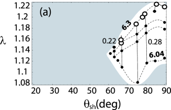
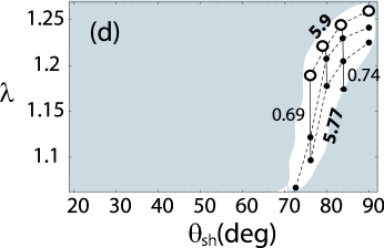
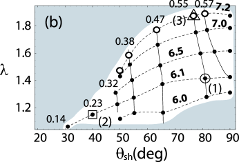
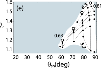
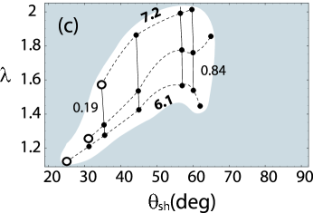
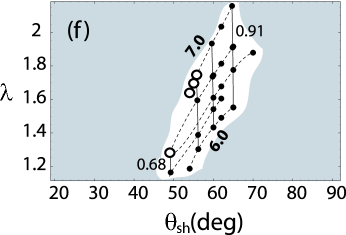
Figure 3: Shock compression ratio $\lambda$ as a function of polar angle $\theta_{\rm sh}$ for various $\hat{E}$ and $\tilde{L}\Omega_{F}$ corresponding to the solutions in Figure 2. The shaded regions represent the regions where no shock-included trans-magnetosonic solutions are possible (forbidden regions) for any $(\hat{E},\tilde{L}\Omega_{F})$ combination for a fixed $(\Omega_{F},\hat{\eta})$. The other notations are the same as in Figure 2.

In a black hole magnetosphere, the magnetic field geometry should in principle be described by the trans-field force balance equation (the Grad-Shafranov equation), which describes the mutual interaction between the frozen-in plasma and the surrounding global magnetic fields. As the plasma generates the toroidal/poloidal current distribution, the poloidal/toroidal magnetic fields are produced and the magnetosphere is constructed. Although solving this trans-field balance equation is an extremely difficult problem, there have been some attempts in the past to study the steady-state magnetospheric configuration around black holes (see, for instance, Mobarry & Loveless 1986 for Schwarzschild geometry and Camenzind 1987 for Minkowski geometry). Nitta, Takahashi, & Tomimatsu (1991) extended these studies to Kerr geometry in order to analytically study a rotating black hole magnetosphere, and found dipole-like fields (see Figure 3b in Nitta, Takahashi, & Tomimatsu, 1991). Tomimatsu & Takahashi (2001) solved a vacuum magnetosphere with a thin equatorial disk and obtained a dipole-like geometry in the disk region and a uniform field geometry along the rotational axis. A similar magnetospheric structure was discussed by Li (2002). However, for the accreting plasma very close to the horizon, it was found that the magnetic field lines are almost radial in the poloidal plane (see, e.g., Hirotani et al. 1992; Komissarov 2005; Uzdensky 2005). Therefore, in our current paper we mostly adopt a conical geometry because we are interested in the accreting plasma very close to the event horizon. However, we will also explore the effect of different magnetic field geometries. Figure 1 schematically illustrates a magnetic field geometry in the poloidal plane adopted in this paper. We explore the possibility of MHD shock formation along the poloidal magnetic field lines, which may illuminate the underlying accretion disk, with possible application to the central engine of AGN in mind. Although the plasma flows can originate from the accreting material in the equator, the exact plasma source can be diverse, and we do not specify them in this paper.

From the standpoint of recent MHD simulations, the past several years have seen the long-awaited advance in numerical general relativistic MHD simulations to study the geometrical nature of the black hole magnetosphere and the dynamical properties of the plasma emersed in the global magnetic fields. These dynamical simulations will help to offer the means to predict the boundary conditions and parameters governing the black hole magnetosphere. For example, Koide et al. (2000) explored the roles of the global magnetic fields coupled with the accreting plasma where the shock formation is found in the equator, while Hirose et al. (2004) analyzed the structure of various magnetic fields around a rotating black hole. The astrophysical processes that influence the spin evolution of black holes are studied by Gammie, Shapiro, & McKinney (2004). Through long time-evolved MHD simulations, McKinney & Gammie (2004) found five main subregions of the black hole magnetosphere in a quasi-steady state at the final simulation time. De Villiers et al. (2005) recently showed that the unbound outflows can emerge self-consistently in the axial funnel region where the large-scale magnetic field spontaneously arises. The structure of large-scale Poynting-dominated jets is discussed by McKinney (2006). On the other hand, in order to gain further physical insights, here we emphasize that parallel more analytic, steady-state investigations should be equally important, and that is a major goal of our current studies.

From X-ray observations of accretion-powered AGNs, particularly Seyfert galaxies, it has become evident that accretion disks play a crucial role in the central high energy activities (e.g., Nandra & Pounds, 1994; Pounds et al., 1994). Rapid instrumental progress of recent X-ray observatories (i.e., Chandra and XMM-Newton) allows us to further investigate the detailed dynamics of accreting plasmas in the immediate environment of supermassive black holes hosted in these AGNs. It has been widely accepted that the gravitational energy of the plasma is viscously dissipated into thermal energy in the course of accretion, producing the signature of thermal emission in the observed spectra in many Seyfert galaxies. Furthermore, the presence of the power-law X-ray continuum component suggests the existence of magnetic fields in/around the accretion disks (see, e.g., Haardt & Maraschi, 1991, for an AGN model). Therefore, in order to better understand the nature of the accreting magnetized plasma near a black hole, it is important to consider the role of both general relativity and magnetic fields. Meier (2004) proposed that the inner part of the ingoing flows may enter a magnetically-dominated, magnetosphere-like phase in some Galactic black hole candidates (GBHCs) (e.g., GRS 1915+105) and perhaps some low-luminosity AGNs (e.g., NGC 6251) as well. His model is based on a strong, large-scale magnetic field structure around a black hole. These issues point to the importance of investigating the basic physics of a high energy source in the black hole magnetosphere. One motivation for our current paper is thus to provide a scenario, in terms of MHD shock formation in inflowing plasmas, that generates hot or magnetized plasma regions very close (within a few gravitational radii) to a black hole.

The structure of this paper is as follows. In §2 we briefly summarize our previous work on MHD shock formation in a rotating black hole magnetosphere and describe the trans-magnetosonic property of the plasma. We also show general relativistic adiabatic MHD shock conditions for the possible parameter space. The parameter dependence of the shock-related quantities is explored in §3, where we study the nature of our shock solutions and shock-included global solutions. We particularly focus on the non-equatorial MHD shock formation, by examining the polar angle dependence and place constraints on possible allowed shock regions in the parameter space. In §4 we discuss our results in terms of a black hole-plasma system coupled to a global magnetic field lines. Brief summary and concluding remarks are given in the last section, §5.

2 Assumptions & Basic Equations

2.1 Black Hole Magnetosphere and MHD Accreting Flows

We consider stationary and axisymmetric ideal MHD accretion flows in Kerr geometry. The background metric is written by the Boyer-Lindquist coordinates with the $c=G=1$ unit,

$$ds^{2} = \left(1-\frac{2mr}{\Sigma}\right)dt^{2}+\frac{4amr\sin^{2}\theta}{\Sigma}dtd\phi$$ (1)

$$-\frac{A\sin^{2}\theta}{\Sigma}d\phi^{2}-\frac{\Sigma}{\Delta}dr^{2}-\Sigma d\theta^{2}\ ,$$

where $\Delta\equiv r^{2}-2mr+a^{2}$, $\Sigma\equiv r^{2}+a^{2}\cos^{2}\theta$, $A\equiv(r^{2}+a^{2})^{2}-a^{2}\Delta\sin^{2}\theta$, and $m$ and $a$ denote the mass and angular momentum per unit mass of the black hole, respectively. We take $m=1$ throughout this paper. The black hole event horizon is $r_{H}\equiv 1+\sqrt{1-a^{2}}$.

In the context of general relativistic ideal MHD, the basic equations governing plasmas consist of: (1) particle number conservation law: $(nu^{\alpha})_{;\alpha}$ where $n$ is the proper particle number density and $u^{\alpha}$ is the plasma four-velocity, (2) equation of motion: $T^{\alpha\beta}_{~{}~{};\beta}=0$ where $T^{\alpha\beta}$ is the energy-momentum tensor for plasmas and (3) ideal MHD condition: $u^{\beta}F_{\alpha\beta}=0$ where $F_{\alpha\beta}$ is the electromagnetic field tensor. We also denote the poloidal plasma velocity as $u_{p}^{2}\equiv-(u^{r}u_{r}+u^{\theta}u_{\theta})$. The energy-momentum tensor $T^{\alpha\beta}$ is given by

$$T^{\alpha\beta}\equiv n\mu u^{\alpha}u^{\beta}-Pg^{\alpha\beta}+\frac{1}{4\pi}\left(F^{\alpha\gamma}F_{\ \gamma}^{\beta}+\frac{1}{4}g^{\alpha\beta}F^{2}\right)\ ,$$ (2)

where $F^{2}\equiv F_{\mu\nu}F^{\mu\nu}$ and $\mu=(\rho+P)/n$ is the relativistic enthalpy, $P$ is the thermal gas pressure and $\rho$ is the total energy density.

For a stationary and axially symmetric ideal MHD plasma, there exist five conserved quantities along a field line: total energy $E$ and angular momentum $L$ of the plasma, angular velocity of the magnetic field line $\Omega_{F}$, particle flux per magnetic flux $\eta$ and entropy $S$ (see Camenzind, 1986, R03). The total energy and angular momentum of the plasma are

$$E \equiv \mu u_{t}-\frac{\Omega_{F}B_{\phi}}{4\pi\eta}\ ,$$ (3)

$$L \equiv -\mu u_{\phi}-\frac{B_{\phi}}{4\pi\eta}\ ,$$ (4)

where $\Omega_{F}\equiv-F_{tr}/F_{\phi r}=-F_{t\theta}/F_{\phi\theta}$ (see Bekenstein & Oron, 1978) and $\eta\equiv nu_{p}/B_{p}$.

In the Boyer-Lindquist coordinates, the toroidal component of the magnetic field seen by a distant observer is defined by $B_{\phi}\equiv(\Delta/\Sigma)F_{\theta r}$, and the poloidal one is defined as $B^{2}_{p}\equiv-[g^{rr}(^{\ast}F_{rt})^{2}+g^{\theta\theta}(^{\ast}F_{\theta t})^{2}]G^{-2}_{t}$ where ${}^{\ast}F_{\alpha\beta}\equiv(1/2)\sqrt{-g}\epsilon_{\alpha\beta\gamma\delta}F^{\gamma\delta}$ is the tensor dual to $F_{\alpha\beta}$ and $G_{t}\equiv g_{tt}+g_{t\phi}\Omega_{F}$. The dynamical timescale of accretion is assumed to be much shorter than diffusion timescale so that the adiabatic prescription is used for the infalling plasma as $P=K\rho_{0}^{\Gamma}$, where $\Gamma$ is the adiabatic index, $K$ is related to entropy $S$. $\rho_{0}=m_{p}n$ is the rest-mass density [i.e., $\rho=\rho_{0}+P/(\Gamma-1)$], and $m_{p}$ is the particle mass. We introduce the so called entropy-related mass-accretion rate (e.g., Chakrabarti, 1990) as

$$\dot{\cal{M}}\equiv m_{p}\eta K^{N}\ ,$$ (5)

the polytropic index $N$ is given by $\Gamma=1+1/N$. Note that $\dot{\cal{M}}=0$ for the cold flow limit (because of $K=0$).

The poloidal equation is given by (see, e.g., Takahashi et al., 1990)

$$\mu^{2}(1+u_{p}^{2})=E^{2}\left[(\alpha-2M^{2})f^{2}-k\right]\ ,$$ (6)

with $f\equiv-(G_{\phi}+G_{t}\tilde{L})/[\rho_{w}(M^{2}-\alpha)]$, $\alpha\equiv g_{tt}+2g_{t\phi}\Omega_{F}+g_{\phi\phi}\Omega_{F}^{2}$, $k\equiv(g_{\phi\phi}+2g_{t\phi}\tilde{L}+g_{tt}\tilde{L}^{2})/\rho_{w}^{2}$, $\tilde{L}\equiv L/E$, $\rho^{2}_{w}\equiv g^{2}_{t\phi}-g_{tt}g_{\phi\phi}$ and $G_{\phi}\equiv g_{t\phi}+g_{\phi\phi}\Omega_{F}=g_{\phi\phi}(\Omega_{F}-\omega)$, where $\omega\equiv-g_{t\phi}/g_{\phi\phi}$ is the angular velocity of a zero angular momentum observer (ZAMO). The relativistic Alfvén Mach number $M$ is defined as

$$M^{2}\equiv\frac{4\pi\mu nu_{p}^{2}}{B_{p}^{2}}=\frac{4\pi\mu\eta u_{p}}{B_{p}}\ .$$ (7)

The toroidal magnetic field $B_{\phi}$ can be expressed as $B_{\phi}=-4\pi\eta E\rho_{w}f$.

Any physical MHD accreting plasma ejected from the plasma source with a small poloidal velocity onto a black hole must become fast magnetosonic at the event horizon, going through three magnetosonic critical points: a slow magnetosonic point (S: $r=r_{\rm S}$ where $u_{p}=u_{\rm SW}$), the Alfv$\acute{e}$n point (A: $r=r_{\rm A}$ where $u_{p}=u_{\rm AW}$) and a fast magnetosonic point (F: $r=r_{\rm F}$ where $u_{p}=u_{\rm FW}$). At each magnetosonic point the plasma speed is equal to each magnetosonic wave speed. Here, $u_{\rm SW},u_{\rm AW}$ and $u_{\rm FW}$ are the slow, the Alfv$\acute{e}$n and the fast magnetosonic wave speed, respectively (see Takahashi et al., 1990, for their definitions). When the preshock flow is cold (i.e., $P=0$ or $\mu=m_{p}$), the ejected plasma is super-slow magnetosonic; the slow magnetosonic point will be absent in the cold flow solution.

The function $f$ becomes zero when the numerator of the expression of $f$, $G_{\phi}+G_{t}\tilde{L}$, is zero. There are one or two radii saisfying this condition and we will denote this radius ($r=r_{\rm A}$) the “Alfv$\acute{e}$n radius”. When the plasma poloidal speed becomes equal to the Alfv$\acute{e}$n speed ($u_{p}=u_{\rm AW}$ or $M^{2}=\alpha$) at this radius, this point is called the “Alfv$\acute{e}$n point”. Otherwise, it is termed the “anchor point” where the toroidal component of the magnetic field $B_{\phi}$ is zero ($M^{2}\neq\alpha$). In the next section, let us apply MHD shock conditions to these accreting plasma flows.

2.2 General Relativistic MHD Shock Conditions

In TRFT02 and Paper I, we discussed in detail general relativistic Rankine-Hugoniot shock conditions in Kerr geometry that apply to accreting plasmas: particle number conservation $[nu^{\alpha}]_{\rm sh}~{}\ell_{\alpha}=0$, energy and angular momentum conservation $[T^{\alpha\beta}]_{\rm sh}~{}\ell_{\alpha}=0$ and magnetic flux conversation $[^{\ast}F^{\alpha\beta}]_{\rm sh}\ell_{\alpha}=0$, where $\ell_{\alpha}$ is the unit vector normal to the shock front. The square brackets denote the difference between the values of a quantity on the two sides of the shock front.

The poloidal magnetic field in our assumption is explicitly given by $B_{p}(r)=C/(\sqrt{\Delta\Sigma}~{}r^{\delta})$ where $C$ is a constant. To investigate the effects of the non-radial poloidal magnetic field, the poloidal field is parameterized by $\delta$: $\delta=0$ for a purely conical field and $\delta>0$ for an outward diverging field. The conical magnetic field with $\delta=0$ is adopted in most of our computations unless otherwise stated. In the following, for simplicity we set the shock front to be normal to the magnetic field lines, $\ell_{\alpha}=(0,1,0,0)$. These conservation laws lead to the following jump conditions:

$$n_{1}u^{r}_{1}=n_{2}u^{r}_{2}\ ,$$ (8)

$$\left(\frac{1}{\sqrt{\Delta\Sigma}~{}r^{\delta}}\right)^{2}M^{2}_{1}+\frac{\hat{\mu}_{1}\hat{\eta}}{M^{2}_{1}}\left[\frac{\hat{\eta}\left(\hat{\mu}_{1}-1\right)}{1+N}\right]+\frac{1}{2}(\hat{\eta}\hat{E})^{2}f^{2}_{1}$$

$$=\left(\frac{1}{\sqrt{\Delta\Sigma}~{}r^{\delta}}\right)^{2}M^{2}_{2}+\frac{\hat{\mu}_{2}\hat{\eta}}{M^{2}_{2}}\left[\frac{\hat{\eta}\left(\hat{\mu}_{2}-1\right)}{1+N}\right]+\frac{1}{2}(\hat{\eta}\hat{E})^{2}f^{2}_{2}\ ,$$ (9)

and the relation:

$$\left(\hat{\mu}\hat{\eta}\right)^{2} = (\hat{\eta}\hat{E})^{2}\left[\left(\alpha-2M^{2}\right)f^{2}-k\right]-\left(\frac{1}{\sqrt{\Delta\Sigma}~{}r^{\delta}}\right)^{2}M^{4}_{2}\ .$$ (10)

where $\hat{\mu}\equiv\mu/m_{p}$, $\hat{E}\equiv E/m_{p}$ and $\hat{\eta}\equiv 4\pi\eta m_{p}/C$. The subscripts “1” and “2” respectively denote the preshock and postshock quantities. The field-aligned conserved quantities ($E,\tilde{L},\Omega_{F},\eta$) are continuous across a MHD shock. Then, our entropy-related accretion rate can be expressed as:

$$\dot{\cal{M}} = \frac{C}{m_{p}}\frac{M^{2}}{\hat{\mu}\hat{\eta}}\left(\frac{\hat{\mu}-1}{1+N}\right)^{N}\ .$$ (11)

Note that $\dot{\cal{M}}$ is continuous in shock-free flow regions, but it is discontinuous across a shock ($\dot{\cal{M}}_{1}<\dot{\cal{M}}_{2}$) because of the entropy generation, where the adiabatic shock is related to extremely inefficient cooling processes. That is, most of the heat generated at the shock front is carried away (advected) with the accreting plasma.

It should be noted from the shock condition expressed by equations (9) and (10) that the plasma energy $\hat{E}$ is coupled with the parameter $\hat{\eta}$ as $\hat{\eta}\hat{E}$, while the angular momentum $L$ is always coupled with $E$ as $\tilde{L}\equiv L/E$ through functions $f$ and $k$. Also, the enthalpy $\hat{\mu}$ in equation (9) frequently appears with $\hat{\eta}$ as $\hat{\mu}\hat{\eta}$, which can be expressed in terms of parameters $\hat{\eta}\hat{E}$, $\tilde{L}$ and $\Omega_{F}$ through equation (10). When the downstream plasma becomes extremely hot (i.e., large $\hat{\mu}_{2}\gg 1$), the coupled parameter, $\hat{\eta}\hat{E}$, acts as a controlling parameter for determining the shock solutions. The equation (9) also shows that the loss of kinetic energy leads to the gain of the (toroidal) magnetic and thermal energy across the fast MHD shocks. Thus, in our computations, we will use the coupled parameter $\hat{\eta}\hat{E}$.

We now introduce some shock-related quantities that are useful for examining the properties of MHD shocks. First, let us define the magnetization parameter $\sigma$, which denotes the ratio of the Poynting flux to the net mass-energy flux of the accreting plasma seen by the ZAMO (see TRFT02). From the ZAMO’s standpoint, $\sigma$ can be written as

$$\sigma\equiv\frac{B_{\phi}g_{\phi\phi}(\Omega_{F}-\omega)}{4\pi\eta\mu u^{t}\rho^{2}_{w}}=-\frac{\tilde{e}-\alpha\tilde{h}}{\tilde{e}-M^{2}\tilde{h}}\ ,$$ (12)

where $\tilde{h}\equiv g^{tt}(1-\omega\tilde{L})$ and $\tilde{e}\equiv 1-\tilde{L}\Omega_{F}$.

The local strength of a shock is measured by the ratio of the postshock to the preshock number density, $n_{2}/n_{1}$, as

$$\lambda\equiv\frac{n_{2}}{n_{1}}\ .$$ (13)

Since any physical shocks that satisfy the second law of thermodynamics must be compressible, we require $\lambda>1$ for physically relevant shock formation. Then, the postshock plasma is heated up. In order to quantitatively evaluate shock heating, we furthermore define a dimensionless postshock plasma temperature $\Theta$ as

$$\Theta\equiv\frac{k_{B}T}{m_{p}}=\frac{\hat{\mu}-1}{1+N}\ ,$$ (14)

assuming the equation of state for an ideal gas (i.e., $P=nk_{B}T$ where $k_{B}$ is the Boltzmann constant and $T$ is the plasma temperature). Notice that $\Theta\ll 1$ for the cold flow ($P_{1}=0$ and $\mu_{1}=m_{p}$). Depending on the temperature $\Theta$, the postshock flow, heated by the shock, may be capable of emitting high energy thermal radiation, although in practice it is also necessary to consider non-thermal radiation due to the magnetic field.

To include the radiative effects on MHD flows, which means the breakdown of ideal MHD approximation, we should formulate the general relativistic version of radiative (non-ideal) trans-magnetosonic flow solutions, where $E,L,\eta,\Omega_{F},\dot{\cal{M}}$ are not conserved along the magnetic field line. However, the task is very complicated, and that is beyond the scope of our present paper. Therefore, we will not include the radiative effects on the postshock hot flows and consider ideal MHD trans-magnetosonic flows.

2.3 Shock-Included Trans-magnetosonic Accretion Flows

In the following we consider the MHD shock formation around a Schwarzschild and slowly-rotating Kerr black hole (i.e., $0\leq\omega_{H}<\Omega_{F}$ where $\omega_{H}\equiv\omega(r_{H})$, see also Paper I). Although the black hole accretes the surrounding gas inward by its strong gravity, there are several mechanisms in general for decelerating the accreting gas: the centrifugal force due to plasma’s angular momentum, magnetic tension and magnetic pressure. For accretion onto black holes a shock can be formed through these obstacles. Detailed studies of this possibility will be a focus of much of this section. We restrict ourselves to cold preshock plasmas which are initially injected from a plasma source (e.g., accretion disk/torus). We impose that the cold plasma starts falling onto the black hole with small poloidal velocity (i.e., $u_{p}<u_{\rm AW}$) from this injection point (I) which is located somewhere between the outer light surface (L) and the Alfv$\acute{e}$n point (A). The exact location of the injection point will be important when considering the boundary conditions of the accreting plasma that should be specified by some accretion disk model, but that is beyond the scope of our present paper.

We should point out the rotational energy per total energy, $\tilde{L}\Omega_{F}$, is one of the useful parameters for predicting the degree of magnetization of the shocked plasma flow. In Paper I we discussed that there is a finite range in the value for $\tilde{L}\Omega_{F}$ in order for the multiple Alfv$\acute{e}$n points to exist for the $\Omega_{F}>\omega_{H}$ case; that is, $(\tilde{L}\Omega_{F})_{\rm min}<\tilde{L}\Omega_{F}<(\tilde{L}\Omega_{F})_{\rm max}$. As the value of $\tilde{L}\Omega_{F}$ becomes larger, the plasma becomes more magnetized because in the energy equation (3) the magnetic term (second term) becomes more effective as $\tilde{L}\Omega_{F}$ increases.

Here, we briefly describe a shock-included trans-magnetosonic accretion flow. The poloidal equation (6) specifies the velocity of a plasma flow for a given set of initial parameters. When a MHD shock develops, both preshock and postshock flow solutions must pass through appropriate critical points: that is, the flow must pass through the fast magnetosonic points twice (outer and inner fast magnetosonic points). As discussed earlier, for a given set of conserved quantities, there exist two Alfv$\acute{e}$n radii : outer and inner Alfv$\acute{e}$n radii for a slowly-rotating black hole case. We consider that an upstream preshock solution goes through the outer Alfv$\acute{e}$n radius while the corresponding downstream postshock solution passes through the inner Alfv$\acute{e}$n radius. The outer Alfv$\acute{e}$n radius is identified as the Alfv$\acute{e}$n point (A) while the inner Alfv$\acute{e}$n radius corresponds to the anchor point for the upstream solution. The anchor point is located somewhere between the outer fast magnetosonic point F_out and the fast MHD shock location. When a shock forms inside the anchor point, the magnetic field line is refracted away from the shock normal. Such a shock is called a fast MHD shock. In fast MHD shocks, the preshock plasma must be super-fast magnetosonic while the postshock plasma must be sub-fast magnetosonic. This postshock plasma must pass through another fast magnetosonic point (F) again before reaching the horizon (H) (i.e., I $\rightarrow$ A $\rightarrow$ F_out $\rightarrow$ Fast Shock $\rightarrow$ F_in $\rightarrow$ H). When a shock forms outside the anchor point, the magnetic field line is flipped over across the shock normal. Such a shock is called an intermediate MHD shock (see, e.g., Hada, 1994; De Sterck & Poedts, 2000, 2001, for its physical significance). In intermediate MHD shocks, the preshock plasma must be super-Alfv$\acute{e}$nic while the postshock plasma must be sub-Alfv$\acute{e}$nic. This postshock plasma must pass through another Alfv$\acute{e}$n point (A) and a fast magnetosonic point (F) subsequently again before reaching the horizon (H) (i.e., either I $\rightarrow$ A_out $\rightarrow$ Intermediate Shock $\rightarrow$ A_in $\rightarrow$ F_in $\rightarrow$ H or I $\rightarrow$ A_out $\rightarrow$ F_out $\rightarrow$ Intermediate Shock $\rightarrow$ A_in $\rightarrow$ F_in $\rightarrow$ H). When a shock occurs right at the anchor point, it is called a “switch-on shock” for which the magnetic field line of the preshock flow is radial. The shock condition (9) determines whether a MHD shock can form for a given field-aligned parameter sets. In such a global accretion solution with a MHD shock, the preshock cold plasma [i.e., $\dot{\cal{M}}_{1}(r_{\rm sh},M^{2}_{1})=0$] is connected to the subsequent postshock hot plasma [i.e., $\dot{\cal{M}}_{2}(r_{\rm sh},M^{2}_{2})>0$] through the shock formation where the Alfv$\acute{e}$n Mach number jumps from $M_{1}$ to $M_{2}$ (see Paper I). In the next section we systematically explore the parameter dependence of the resulting MHD shocks by varying certain primary quantities.

3 Numerical Results

In this section, the shock-included trans-magnetosonic accretion solutions are solved in wide ranges of field-aligned flow parameters, where slowly-rotating black hole cases are considered; that is, the magnetic field lines in the black hole magnetosphere rotate faster than the black hole itself. In this case, there are two Alfv$\acute{e}$n  radii on the $r$-$M^{2}$ plane. The locations are specified by the two field-aligned parameters, namely $\Omega_{F}$ and $\tilde{L}$. These parameters $\Omega_{F}$ and $\tilde{L}$ have the minimum and maximum values for allowing the Alfv$\acute{e}$n  radii. These values depend on the geometry of magnetic field lines. In our assumed conical field configuration, these values depend on the polar angle $\theta$. We must change the values of $\Omega_{F}$ and $\tilde{L}$ in the acceptable range in order to search for physical solutions. AC88 and R03 both have suggested that $\Gamma=4/3$ is not a good approximation even for large radial velocity. In many fast shock cases, R03 has found that $\Gamma\sim 3/2$ (i.e., $N\sim 2$). Following their claim, we choose $\Gamma=3/2$ ($N=2$) in this paper. We have checked that this choice is not qualitatively too critical for our end results.

As to the choice of field-aligned parameter sets for computations, there are additional three restrictions for selecting our parameters: regularity conditions at the outer and inner fast magnetosonic points and the shock condition connecting preshock and postshock trans-magnetosonic flows. Three out of five conserved parameters are related by these restrictions. Consequently, for a given black hole spin $a$ and the magnetic field line with polar angle $\theta_{\rm sh}$, the shock location $r_{\rm sh}$ is determined when the five parameters are selected in the acceptable parameter range, and the corresponding shock quantities are obtained. If we modify one of the parameters [i.e., the field-aligned parameters ($E,L,\eta,\Omega_{F}$) + geometrical parameters $(a,r_{\rm sh},\theta_{\rm sh},\delta)$], to find another global shock solution, we must change at least one more field-aligned parameter. Therefore, to clarify the $\theta_{\rm sh}$-dependence of MHD shock solutions, we change one parameter at a time in such a way that the degeneracy in shock solutions is removed. This allows us to systematically examine each parameter-dependence of the shock solutions. As explained in section §2.2, the shock condition in equation (9) is conveniently characterized by $\hat{\eta}\hat{E}$ and $\tilde{L}\Omega_{F}$, and therefore in the rest of the computations we will basically use $\hat{\eta}\hat{E}$ and $\tilde{L}\Omega_{F}$ as control parameters.

3.1 Non-equatorial MHD Shock Solutions

We first show in Figure 2 the possible shock region in the poloidal plane ($r_{\rm sh},\theta_{\rm sh}$) for different ($\hat{E},\tilde{L}\Omega_{F}$) sets, where we can uniquely obtain a point on the poloidal plane ($r_{\rm sh},\theta_{\rm sh}$) for a set of $(\hat{E},\tilde{L}\Omega_{F})$. (a) $\Omega_{F}=0.1$, (b) $0.14$, and (c) $0.2$ for the $a=0$ case and (d) $0.21$, (e) $0.22$ and (f) $0.25$ for the $a=0.5$ case. Along each curve in these figures, either $\hat{E}$ or $\tilde{L}\Omega_{F}$ is fixed while the other parameter (either $\tilde{L}\Omega_{F}$ or $\hat{E}$) is varied, as indicated by the numbers. For a more detailed discussion of the global nature of the trans-magnetosonic accretion solutions, we select some representative shock solutions. The labels (1)-(3) denote the selected models: the model (1) near-equatorial shock, the model (2) mid-latitude shock with the same energy as (1), and the model (3) near-equatorial shock with larger energy. See Table 1 for the characteristic parameters for these models. As mentioned in §2 the shock location $r_{\rm sh}$ is constrained by the shock condition in equation (9) and the trans-magnetosonic property.

Here, we should mention that, in the black hole magnetosphere with a given black hole spin $a$ and magnetic field distribution $\delta$, we can obtain the cubic parameter space ($\hat{E},\tilde{L}\Omega_{F}$ and $\Omega_{F}$), and the dependence of various shock solutions [e.g., $\lambda(\theta_{\rm sh})$] on $\hat{\eta}$ is not focused here since we find that it is very weak compared with the other parameters. This is because $\hat{\eta}\hat{E}\sim$ constant once $\tilde{L}$ and $\Omega_{F}$ are specified. That is, larger (smaller) $\hat{\eta}$ and smaller (larger) $\hat{E}$ yields roughly the same shock solutions for a fixed $\tilde{L}\Omega_{F}$ (see Paper I for details). We thus show the possible shock parameter space by $\hat{E}$ instead of $\hat{\eta}\hat{E}$ and use a certain specified constant $\hat{\eta}$-value to plot the diagram. Figure 2 is a map of this cubic parameter space onto the ($r_{\rm sh},\theta_{\rm sh}$) plane, corresponding to a slice of such a cubic parameter space by the $\Omega_{F}=$constant planes. Thus, under the considered magnetosphere, physically valid MHD shocks are restricted to this cubic space.

As $\hat{E}$ increases, the shock location $r_{\rm sh}$ tends to shift further out for a given specific angular momentum $\tilde{L}$. This is because the upstream plasma with very large $\hat{E}$ generally means large kinetic energy, too, making it easier for the fluid speed to exceed the magnetosonic speed. Similar results are obtained in the HD shock formation (see, Lu & Yuan 1998 for the equatorial shocks and FT 2004 for the non-equatorial shocks). Then, the shock can form sooner (i.e., further out). In order for accretion to effectively operate near the mid to high latitudes, the specific angular momentum $\tilde{L}$ needs to decrease to reduce the centrifugal force. The accretion cannot take place otherwise. We have confirmed in separate calculations that larger $\Omega_{F}$ can allow the MHD shocks to form closer to the rotation axis with $\theta_{\rm sh}$ as small as $\sim 5\arcdeg$.

Next, let us examine the parameter space that allows the shock formation. In Figure 3 we display (fast and intermediate) MHD shock solutions for various energy $\hat{E}$, specific angular momentum, $\tilde{L}$ and polar angle $\theta_{\rm sh}$ for fixed angular velocity of the field line $\Omega_{F}$. It is first noted that the allowed shock region is continuous but limited in the parameter space. For a given set of $(\hat{E},\tilde{L}\Omega_{F})$ the shock strength $\lambda$ generally becomes stronger as $\theta_{\rm sh}$ increases (i.e., the closer to the equator, the stronger the shocks). This is also seen in the non-equatorial HD shocks (see FT04). The obtained qualitative pattern appears to be independent of the choice of $\Omega_{F}$ and the black hole spin $a$ (compare the left and right columns in Figure 3). We find that there exists the allowed region for the shock formation in the parameter space spanned by ($\hat{E},\tilde{L}\Omega_{F}$) for a fixed $\Omega_{F}$ and a given magnetosphere model. Outside the allowed region (shaded region), physically valid shock solutions disappear for the two reasons: (i) the shock condition by equation (9) is no longer met as $\hat{E}$ decreases (see, e.g., Paper I) and (ii) the inner fast magnetosonic point disappears as $\hat{E}$ increases. That is, as you slice the entire parameter space along a constant $\tilde{L}\Omega_{F}$-curve as in Figure 3, there exists a definite border line between the shock allowed and forbidden regions determined by either condition (i) or (ii) depending on the $\tilde{E}$-value. Additionally, there is a constraint on the parameter space in terms of the existence of the Alfv$\acute{e}$n point. Because the parameter space allowed by the requirement of the Alfv$\acute{e}$n point is wider than those by the conditions (i) and (ii), the allowed shock region shown in Figure 3 satisfies all the conditions by (i), (ii) and the Alfv$\acute{e}$n point.

In general we have confirmed that the minimum value of $\theta_{\rm sh}$ is determined by the above condition (i) while the maximum value of $\theta_{\rm sh}$ by the condition (ii). For accretion to take place in higher latitude regions (i.e., smaller $\theta_{\rm sh}$), the angular velocity of the field line $\Omega_{F}$ is forced to increase. Because the range of $\tilde{L}\Omega_{F}$-value is restricted by the existence of the Alfv$\acute{e}$n points on the shock-included trans-magnetosonic accretion solution (see Paper I for details), $\Omega_{F}$ must increase as $\tilde{L}$ decreases in higher latitude regions for a shock to occur, where $\tilde{L}\propto\sin^{2}\theta_{\rm sh}$. Thus, the allowed region in Figure 3 topologically shifts as $\Omega_{F}$ changes. That is, the shock is allowed more in the mid-high latitudes as $\Omega_{F}$ increases. In other words, high latitude shock formation can only be allowed by large $\Omega_{F}$. In this case, the shock tends to become stronger with increasing $\Omega_{F}$. This feature, due to the rotation of the magnetic field line, is a new aspect inherent to the MHD shocks which would not exist in the HD shock properties. We have obtained diagrams similar to Figure 3 for different $\hat{\eta}$-values and find that the $\hat{\eta}$-dependence of the shock solutions is very weak. As to the dependence on energy $\hat{E}$, it is apparent that the shock strength $\lambda$, for instance, is very sensitive to the change in $\hat{E}$ [see, e.g., the models (1) and (3) along the solid curve]. On the contrary, changing $\hat{E}$ under the fixed $\tilde{L}\Omega_{F}$ value has only a weak effect on shifting the polar angle $\theta_{\rm sh}$. For a given $\hat{E}$, the shock can occur over a wide range of angle $\theta_{\rm sh}$ [see, e.g., the models (1) and (2) along the dashed curve].

The topological nature of the parameter space for $a=0.5$ is essentially the same as for the $a=0$ case (compare the left and right columns in Figure 3), in the sense that larger $\Omega_{F}$ allows stronger shocks near the higher latitude regions. However, for rotating black holes the shock region does not reach as high latitudes as for non-rotating ones. We have also found that the black hole spin $a$ generally amplifies the shock strength as in the HD shocks. However, the coupling among various parameters in the presence of the magnetic field complicates the situation. Around a rotating black hole, it is seen that the allowed region in the polar direction appears to be narrower compared with the $a=0$ case (compare the left and right columns in Figure 3). This is because there is a tighter constraint on the value for $\tilde{L}\Omega_{F}$ (not for $\eta E$) that allows shock formation. This is explained by considering the presence of the Alfv$\acute{e}$n point on the accretion solution. Because the location of the Alfv$\acute{e}$n point is determined by $\tilde{L}\Omega_{F}$, as $a$ changes, the allowed range of $\tilde{L}\Omega_{F}$ is varied (narrowed down) for the Alfv$\acute{e}$n point to exist on the accretion solution (Takahashi et al., 1990). This black hole spin effect for the Alfv$\acute{e}$n point location is seen in Figure 3 for the allowed shock location.

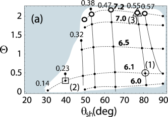
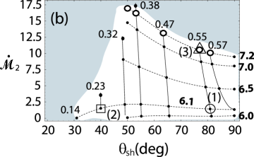
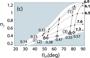
Figure 4: Other shock quantities as a function of $\theta_{\rm sh}$ corresponding to the solutions in Figure 2b: (a) Shocked plasma temperature $\Theta$, (b) postshock entropy-related accretion rate $\dot{\cal{M}}_{2}$, and (c) postshock magnetization parameter $\sigma_{2}$. The notations are the same as in Figure 2.

We present other various shock properties for the postshock flows in Figure 4; (a) shocked plasma temperature $\Theta$, (b) postshock entropy-related accretion rate $\dot{\cal{M}}_{2}$ and (c) postshock magnetization $\sigma_{2}$. The shock solutions marked by (1)-(3) in Figure 4 correspond to the models (1)-(3) in Figure 2b. Temperature $\Theta$ strongly depends on $\hat{E}$. With increase of $\hat{E}$, the temperature can rise significantly [e.g., compare the models (1) and (3)]. The $\dot{\cal{M}}_{2}$ vs. $\theta_{\rm sh}$ behavior is roughly similar to the $\Theta$ vs. $\theta_{\rm sh}$ behavior, except that there is a peak angle in the mid-latitude. On the other hand, the downstream magnetization $\sigma_{2}$ acts quite differently from the other two. With small increase of $\hat{E}$, $\sigma_{2}$ decreases significantly [compare the models (1) and (3)]. That is, $\Theta$ and $\sigma_{2}$ show a clear anti-correlation, as expected from the conserved energy equation (3). We also see a trend that the equatorial shocked plasmas are generally more magnetized than the non-equatorial ones. In separate calculations, we have confirmed that increasing $\Omega_{F}$ will amplify the downstream magnetization $\sigma_{2}$ while it will reduce temperature $\Theta$. Furthermore, in Figure 4c for a fixed $\hat{E}$ the downstream magnetization $\sigma_{2}$ becomes larger as the $\tilde{L}\Omega_{F}$-value becomes larger. Therefore, this is a good indicator for estimating the degree of magnetization of the shocked plasma.

In §2.2 we assumed conical magnetic fields, which would be reasonable around a black hole. However, the magnetospheric configuration other than the $\delta=0$ case may be possible, where $\delta$ parameterizes the cross-section of the magnetic flux. Therefore, we will here explore the effects caused by some other magnetic field configurations. Figure 5 illustrates the dependence of shock strength $\lambda$ on $\delta$. The pure split-monopole field geometry on the poloidal plane is realized with $\delta=0$, while the outward divergent poloidal field is parameterized by $\delta>0$. We find that the MHD shock tends to become stronger as $\delta$ becomes larger. This is because for $\delta>0$ the accreting plasma is more accumulated (or concentrated) toward a smaller cross-sectional area with decreasing $r$ due to the tapered magnetic field. With increasing $\delta$, the accreting plasma in such a field geometry would also become slower. Furthermore, the outward magnetic pressure would be more effective in that case. A larger deviation from a purely radial field configuration tends to not only allow the stronger fast shock $\lambda$, but also enhance the shocked plasma temperature $\Theta$. Note that the increase in $\delta$ shifts the inner fast magnetosonic point inward, while the outer one remains almost the same (Takahashi, 2002). The valid shock location must lie between these outer and inner fast magnetosonic points. Since the location of the fast magnetosonic points shift as $\delta$ changes, the allowed shock location also changes.

3.2 Properties of the Shock-Included Trans-Magnetosonic Solutions

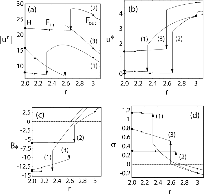
Figure 6: Shock-included trans-magnetosonic accretion solutions as a function of radius $r$: (a) the radial four-velocity $u^{r}$, (b) the toroidal four-velocity $u^{\phi}$, (c) the toroidal magnetic field $B_{\phi}$, and (d) the magnetization parameter $\sigma$. The MHD shock in the accretion solution (vertical downward arrow) is formed after the preshock solution passes through the outer fast magnetosonic point, F_out. The postshock solution then passes through the inner fast magnetosonic point, F_in, and falls onto the event horizon, H. The solutions labelled (1)-(3) correspond to the models (1)-(3) in Figure 2b. See Table 1 for the model parameters.

In this section we consider the global, shock-included trans-magnetosonic solutions for the selected cases [i.e., models (1)-(3)]. We present in Figure 6 several representative solutions, where the models (1)-(3) are selected from Figure 2b. That is, the model (1) near-equatorial shock, the model (2) mid-latitude shock with the same energy as the model (1) and the model (3) near-equatorial shock with greater energy. These inflows all start from several Schwarzschild radii.

The model (1) shows a relatively small downstream kinetic motion [i.e., $|u^{r}_{2}(r)|$ and $u^{\phi}_{2}(r)$] whose magnitude almost remains the same until reaching the event horizon, meaning that the external forces are balanced with the gravity (see Figure 6a and b). For the total energy to be conserved, a large fraction of the total energy then needs to be redistributed to somewhere else. In the model (1), the major part of the energy is redistributed to the magnetic field across the shock, and the postshock magnetization $\sigma_{2}(r)$ is relatively large ($\sigma_{2}\sim 1.1$ in Figure 6d), while the shocked plasma temperature is not high ($\Theta\sim 0.5$ in Figure 4a). Such an anti-correlation is expected from the shock properties shown in Figure 4. Note that $|B_{\phi 1}(r_{\rm sh})|<|B_{\phi 2}(r_{\rm sh})|$, as expected, for the fast MHD shock.

The model (2) has the same energy as the model (1) except for a smaller angular momentum $\tilde{L}$ at $\theta_{\rm sh}=40\arcdeg$. Since the toroidal magnetic field near the event horizon scales as $B_{\phi}\sim B_{\phi,H}\propto\sin^{2}\theta_{H}$ where the subscript $H$ denotes the event horizon, smaller $|B_{\phi,2}|$ is required for the model (2) as seen in Figure 6c. In this case, the magnetic component of energy is accordingly smaller, and the postshock magnetization $\sigma_{2}(r)$ behaves as shown in Figure 6d. To compensate for a smaller magnetic energy component, postshock kinetic energy becomes relatively larger (see Figure 6a). As a result, heating is not significant ($\Theta\sim 0.3$ in Figure 4a). We also find that the shock location $r_{\rm sh}$ shifts outward and in higher latitude regions as in the HD case (see FT04). For example, as $\theta_{\rm sh}$ changes from $81\arcdeg$ in the model (1) to $40\arcdeg$ in the model (2), the shock location shifts outward from $r_{\rm sh}=2.3$ to $2.7$ (see Table 1). This is because the centrifugal force barrier becomes stronger as $\theta_{\rm sh}$ decreases.

As we discussed in the previous sub-section, in Figure 6 the value of $\tilde{L}\Omega_{F}$ is larger in the model (1) than that in the model (2) for a fixed $\hat{E}$. The downstream magnetization parameter $\sigma_{2}(r)$ in Figure 6d is thus greater in the model (1), meaning that the model (1) shows the more magnetized downstream plasma.

For the model (3) we choose a larger energy, $\hat{E}=7.2$ to see the energy dependence of the shock solution. For comparison, the values for the angular momentum and the polar angle are roughly kept the same as in the model (1). Despite the larger total energy, the toroidal magnetic field strength at the event horizon $|B_{\phi,H}|$ has a similar value to that in the model (1) because of the boundary condition at the event horizon. The energy at the shock front in this case is then redistributed more to the thermal and kinetic energies. In fact, we see that the downstream radial acceleration $|du^{r}_{2}(r)/dr|$ is larger, and the downstream toroidal velocity $u^{\phi}_{2}(r)$ is also larger, compared with the models (1) and (2). As expected from Figure 4a, highly heated plasma flow ($\Theta\gtrsim 2$) is realized.

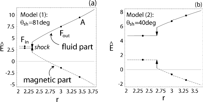
Figure 7: Radial profile of the energy distribution of $\hat{E}$ for models (1) and (2) in Figure 2b. (a) $\tilde{L}\Omega_{F}=0.55$ for the model (1) and (b) $0.23$ for the model (2). See Table 1 for the model parameters in detail.

Next, we will examine the energy distribution of the plasma to further understand the nature of the shocked plasma flows. In Figure 7 we show the components of energy of the plasma, namely fluid $E_{\rm fluid}$ [first term of the right-hand-side in equation (3)] and magnetic $E_{\rm magnetic}$ [second term of the right-hand-side in equation (3)] components, for models (1) and (2) in Figure 2b. In the course of accretion the energy transport between the fluid ($E_{\rm fluid}$) and the magnetic field ($E_{\rm magnetic}$) occurs. Hirotani et al. (1992) discussed the energy transport (or energy redistribution of the plasma) between the two components in shock-free accreting MHD plasmas. In a slowly-rotating black hole case ($0\leq\omega_{H}<\Omega_{F}$), the dominant component in $E$ is fluid energy (i.e., $E_{\rm fluid}>E_{\rm magnetic}$), but the magnetic component can become comparable to or exceed the fluid component near the event horizon for lager $\tilde{L}\Omega_{F}$-value. [see the model (1)]. Note that after the shock each component almost remains unchanged. In other words, the shock acts in such a way that this energy transport from the fluid to the magnetic field is even enhanced at the shock front.

4 Discussion

In order to explore a general trend for MHD shock formation for the vast amount of parameter sets, we sliced the entire parameter space which consists of all of the parameters ($E,L,\Omega_{F},\eta,r_{\rm sh},\theta_{\rm sh};a,\delta$), by finding the allowed cubic parameter space consisting of three parameters ($E,L,\Omega_{F}$), for given black hole magnetosphere models with the other two parameters $a$ and $\delta$ fixed. Since it is very hard to explore all the parameter space spanned by all of the parameters together, our current approach greatly simplifies and yet help us better understand a comprehensive picture of the resulting shock solutions. Through our search for possible non-equatorial MHD shocks we find that the allowed shock region is constrained by various physical factors - especially the regularity conditions at the magnetosonic points and the shock conditions. Because the mathematical expressions for the regularity conditions for the existence of the Alfv$\acute{e}$n  and fast magnetosonic points are not at all simple (e.g., Takahashi, 2002), the topological appearance of the obtained shock regions (see, e.g., Figure 3) is complicated, but nevertheless we find it very useful.

We find in general that stronger MHD shocks can form when the plasma energy is larger. With magnetosphere rotation the shock becomes stronger. The shocked plasma temperature has a clear anti-correlation with the shocked plasma magnetization. The more strongly magnetized plasma is formed for larger $\tilde{L}\Omega_{F}$. We also find that the energy transport between the fluid and the magnetic field can operate even more effectively across the shock front. This transition is internally caused by the transport between these components. Near the equatorial regions the shock is generally stronger. It is thus possible for the astrophysical accreting plasma that very powerful MHD shock formation takes place near the the equatorial event horizon. In the present calculations non-equatorial MHD shocks are possible up to high latitudes with $\theta_{\rm sh}$ as small as $\sim 25\arcdeg$. We found in separate calculations that $\theta_{\rm sh}$ can be as small as $\sim 5\arcdeg$ when $\Omega_{F}$ is sufficiently large. If the poloidal magnetic field or resulting shock is dynamically unstable and switched on and off as the rotating plasma continues to fall onto the event horizon, some sort of quasi-periodic phenomena, perhaps with the dynamical frequency of $\Omega(r_{\rm sh})$ may be expected (where $\Omega\equiv u^{\phi}/u^{t}$ is the angular frequency of the shocked fluid). On the other hand, particles (primarily thermal electrons) would be accelerated at the shock front through first-order Fermi mechanism (Fermi, 1949; Baring, 1997; Gieseler & Jones, 2000) in the presence of the randomly-distributed, turbulent magnetic field. The shock front could then be partly responsible for generating the base of the relativistic winds/jets (e.g., Quataert & Loeb, 2005, for the stellar wind case).

When considering ingoing flows, we adopt mostly a split-monopole poloidal field geometry near the horizon (e.g., Blandford & Znajek, 1977), to mimic the radial magnetic field lines very close to the horizon (see Figure 1). Based on the ideal MHD conditions, the ingoing plasma is assumed to be frozen-in to the magnetic field lines. The ingoing plasma we considered in this work needs to be injected from some plasma sources. Although we do not consider the exact origin of such sources, there are some possible sites for generating the ingoing plasma; e.g., the surface of the accretion disk and/or its corona. In this case, the magnetic field lines connecting to the black hole may come from the outer plasma sources at large radii. Although we consider the conical field lines near the horizon, the poloidal field line can also be bent toward the equator and be connected to the equatorial accretion disk at regions further away from the black hole. We expect that such regions are at least outside the potential well of the particle’s effective potential. Note that in the description of the steady-state black hole magnetosphere, the global poloidal field coupling the black hole event horizon to the surface of a geometrically-thin disk has already been considered (e.g., see Nitta, Takahashi, & Tomimatsu 1991; Tomimatsu & Takahashi 1991 for the analytic solutions, and Komissarov 2005; Uzdensky 2005 for the numerical results). The poloidal field configuration adopted in our model is based on these studies.

In this paper, a typical value for the angular velocity of the field line $\Omega_{F}$ which allows MHD shock formation is about twice that of the Keplerian disk $\Omega_{\rm Kep}(r_{\rm ms})$ (where $r_{\rm ms}$ is the the innermost radius). That is, if the black hole-disk connecting field lines are considered under the conventional Keplerian motion, adiabatic standing MHD shock formation is less likely to occur. Our results suggest that the shock may develop if the rotation of the magnetic field is super-Keplerian [i.e., $\Omega_{F}>\Omega_{\rm Kep}(r_{\rm ms})$] due to some processes. Although we may speculate on what this additional process may be, that is beyond the scope of our current paper. McKinney & Gammie (2004) compared near-equatorial stationary MHD inflows with their time-dependent numerical results between the innermost stable circular orbit and the event horizon. In their inflow solution, there is no MHD shock when the time-averaged numerical value of $\Omega_{F}$ is about $10\%$ of the $\Omega_{\rm Kep}(r_{\rm ms})$. Their result is consistent with our condition for the MHD shock formation; that is, no shock solution exists for $\Omega_{F}\lesssim\Omega_{\rm Kep}(r_{\rm ms})$.

We now show that the values of various primary parameters we chose are not arbitrary, but they are chosen with possible applications to the central engines of AGNs in mind. For instance, for a typical magnetic field strength of AGNs, Krolik (1999) estimates the magnetic field strength as $B\sim 4\times 10^{3}\times T^{2}_{5}$ G under the equipartition assumption where $T_{5}$ is the effective temperature of the disk in units of $10^{5}$ K. For radio-loud narrow-line quasars, Wang et al. (2001) suggests that the field strength of at least $B\sim 10^{4}$ G is required for magnetic-heated corona to operate. Following their implications, we took a likely value of $B_{p}\sim 10^{4}$ G for a typical accretion-powered Seyfert nuclei ($M_{BH}\sim 10^{7}M_{\odot}$) in our estimate. Some of the primary field-aligned parameters are $\tilde{L}$ and $\hat{\eta}$. The physical value for the specific angular momentum $\tilde{L}$ must lie in a certain range in such a way that the Alfv$\acute{e}$n points do exist (see Paper I for details). Since we consider the trans-magnetosonic flows, our choice of $\tilde{L}$ should be reasonable. $\eta$ tells us the particle flux per magnetic flux. Using a commonly used value for the mass-accretion rate for Seyfert nuclei (from observational estimates), $\dot{M}_{acc}\sim 10^{-2}M_{\odot}$/year $\sim 10^{24}$ gram/sec, we can estimate $\hat{\eta}$-value as $\hat{\eta}\sim\dot{M}rc^{2}/C^{2}$ (in physical units) at the horizon. Note that we only take 1% of $10^{24}$ gram/sec for ”our” non-equatorial MHD plasma flows. That is, $\dot{M}_{plasma}\sim 0.01\dot{M}_{acc}\sim 10^{22}$ gram/sec. This is because the plasma density of the non-equatorial flows should be considerably lower than that of the equatorial flows. Also, we have $B_{p}\sim C/r^{2}$, $\eta\equiv nru^{r}c/B_{p}$, and $\dot{M}_{plasma}\sim r^{2}u^{r}nm_{p}$. By eliminating $u^{r},m_{p},\eta$ from these equations, we get $\hat{\eta}\sim r\dot{M}_{plasma}c^{2}/C^{2}\sim 0.01$, which is in the range of values adopted in our calculations. Note also that the estimated value of $\hat{\eta}$ depends on the values of the black hole mass and the magnetic field strength. Depending on these values, $\hat{\eta}$-value can be smaller or larger than $0.01$ by orders of magnitude.

Also, in an attractive model of accretion-powered AGNs, the critical outer region of the disk where the inflowing plasma originates is also where the outflowing plasma is injected. For the outgoing flows, the Lorentz factor $\gamma$ of the observed relativistic jets/winds is generally $\hat{E}=\hat{E}_{\infty}\sim\gamma\sim 10$ (for microquasar black hole systems) to $\gamma\gtrsim 100$ (AGNs and Gamma Ray Bursts (GRBs)) (e.g., Meier, 2003). That implies the presence of highly energetic plasmas being accelerated within the black hole magnetosphere. Because they are injected to form the jets/winds with such high observed energy, $\hat{E}_{\infty}$, the ingoing plasmas also should initially possess the same order of magnitude of energy $\hat{E}\sim\hat{E}_{\infty}$ at the time of their launch from the foot points on the accretion disk. Therefore, the original energy of the MHD flow can also be $\hat{E}\sim 10-100$. A major part of the energy can be magnetic in this case near the plasma source on the disk. Our selected value for $\hat{E}$ ($\hat{E}>1$) in our calculations is then justified. For completeness, we would like to mention that no plasma energetically bound to the black hole (i.e., $\hat{E}\lesssim 1$) appears to get shocked in our case.

We are aware of the degeneracy of our solutions, i.e., the coexistence of shock-free and shock-included solutions for the same set of conserved quantities. To further investigate which steady-state solution between the two is physically accessible in nature, we will need to perform a dynamical analysis by considering a time-dependent perturbation in the flow. Such an analysis is beyond the scope of this paper. However, we may note that some authors (e.g., Ferrari et al., 1984; Trussoni et al., 1988; Nobuta & Hanawa, 1994) have already carried out such an analysis (no magnetic field in a flat space) and concluded that some shock-included solutions are indeed preferred (physically accessible by nature) to the corresponding shock-free solution. That finding probably justifies the motivations of our current work.

Our current investigations carried out through the analytical methods can help gain deeper insight when compared with the results obtained by long dynamical MHD simulations. For instance, when the numerical experiments for black hole magnetospheres are studied under various initial conditions, the MHD shock front may be generated in some computational domain after a long calculation time to a quasi-steady state. Then, we can compare the field-aligned flow parameters for MHD shock formation in our analytic studies with the final values of the corresponding physical quantities obtained by the numerical simulations.

Recently, long-time dynamical evolution of magnetized plasma accretion onto a black hole has been extensively studied, and the global poloidal magnetic fields are obtained by some authors (e.g., Hirose et al., 2004; McKinney & Gammie, 2004; De Villiers et al., 2005; McKinney, 2006). The magnetic field confined in the funnel region is evolved to quasi-steady states at later times, while the magnetic field in the corona and disk fluctuates in magnitude and its direction. Our results may apply to some regions during such a quasi-steady-state in late simulation times. However, the accreting flows (whether equatorial or non-equatorial) are expected to be turbulent, and hence our analysis here, based on axisymmetry and stationary assumptions, is not exactly applicable for explaining short timescale local turbulence in these regions. With this in mind, it is still important to compare our results with the future large-scale MHD simulations in order to better understand the physics in these complex regions.

5 Summary and Concluding Remarks

In Paper I we showed that the MHD shock formation can occur in the equator. In the present work we extended that work to the non-equatorial two-dimensional geometry. We systematically explored, for the first time, general relativistic MHD shock formation in such a geometry by employing the conserved quantities, and found the allowed shock regions. In summary we find that non-equatorial MHD shocks can form and could be a plausible candidate for generating a hot or strongly magnetized region over various latitudes in the non-equatorial plane.

In various astrophysical objects, high energy activities are often associated with the magnetic fields along which the accreting plasma flows. Our investigation of MHD standing shock formation will be useful for our better understanding of complicated interactions between the plasma and the magnetic field in these situations. In the context of a strong radiation source required for the accretion-powered central engines of objects such as AGNs and GBHCs, the presence of non-equatorial shocks therefore can be attractive as a candidate for such a source, and therefore our current work may turn out to be very interesting for future observations of these objects also.

Before closing, it may be emphasized that our search for the parameter space which allows MHD shock formation is carried out in a systematic manner in such a way that our choice of the parameter sets is not arbitrary. It is consistent, for instance, with the numbers relevant in application to, e.g., the environment of black hole magnetospheres around supermassive black holes in AGNs. Within this context, our results are quite general. However, it may be noted that in reality the MHD shock location in the actual astrophysical situation would probably trace a certain trajectory, rather than occupying the whole allowed shock region in the constrained parameter space, because the parameters allowing the shock formation may be unique from case to case. Our hope is that our current studies, through analytic and steady-state analysis, are very useful, because they can be complementary to those with time-dependent numerical simulations, in the sense that the latter can take advantage of, for instance, the constrained parameter space found with our current studies.

Table 1: Characteristics of models (1), (2) and (3) with different $(\hat{E},\tilde{L})$ in Figure 2. $a=0,\delta=0,\Omega_{F}=0.14$ and $\hat{\eta}=0.006$ for all cases.

Model	Symbol	$\hat{E}$	$\tilde{L}$	$\theta_{\rm sh}$	$\lambda$	$r_{\rm sh}$	$\Theta$	$\sigma_{2}$	$\dot{\cal{M}}_{2}$
(1)	$\bigcirc$	6.1	3.9	$81\arcdeg$	1.41	2.3	0.46	1.13	1.31
(2)	$\square$	6.1	1.6	$40\arcdeg$	1.15	2.7	0.29	0.29	1.51
(3)	$\bigtriangleup$	7.2	3.9	$77\arcdeg$	1.91	2.6	2.12	0.45	10.2

Figure 1: A schematic picture of standing MHD shock formation in black hole accretion flows where the poloidal magnetic field lines near the event horizon can be approximated to be radial (not drawn to scale). Note that non-equatorial ingoing MHD plasmas, originating from some plasma sources, are made possible in the presence of the poloidal magnetic fields. The Alfv$\acute{e}$n point, outer and inner fast magnetosonic points (dotted curves) are labelled by A, F_out and F_in, respectively.

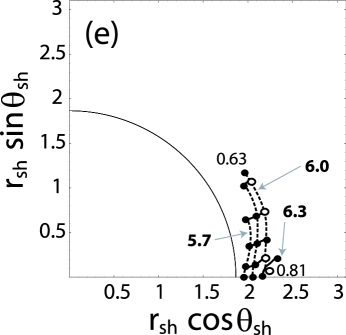
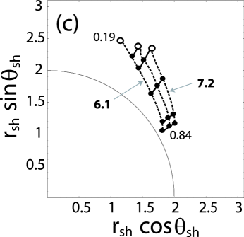
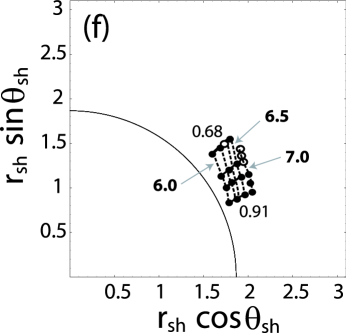
Figure 2: Acceptable parameter space for possible MHD shock formation on the $r_{\rm sh}$-$\theta_{\rm sh}$ plane spanned by parameters ($\hat{E},\tilde{L}\Omega_{F}$). The filled circles ($\bullet$) represent the fast MHD shocks while the open circles ($\circ$) denote the intermediate MHD shocks. We choose (a) $\Omega_{F}=0.1$, (b) $0.14$ and (c) $0.2$ in the left column for $a=0$ and $\hat{\eta}=0.006$, while (d) $\Omega_{F}=0.21$, (e) $0.22$ and (f) $0.25$ in the right column for $a=0.5$ and $\hat{\eta}=0.005$. Solid curves labelled by the thin numbers denote constant $\tilde{L}\Omega_{F}$-curves, while dashed curves labelled by bold numbers denote constant $\hat{E}$-curves. The labels (1)-(3) in (b) denote the selected models. See Table 1 for the characteristic parameters for these models.

Figure 5: The dependence of the shock strength $\lambda(r_{\rm sh})$ on $\delta$ for $\hat{E}=6.1,\tilde{L}=4.1$ and $a=0$. We set $\hat{\eta}=0.006$ for $\delta=0$, $\hat{\eta}=0.003$ for $\delta=1$ and $\hat{\eta}=0.001$ for $\delta=2$. The crosses ($\times$) denote the anchor points. The intermediate MHD shocks are obtained to the right of the anchor points.

References

- Appl & Camenzind (1988) Appl, S., & Camenzind, M., 1988, A&A, 206, 258 (AC88)
- Baring (1997) Baring, M. G. 1997, astro-ph/9711177
- Bekenstein & Oron (1978) Bekenstein, J. D., & Oron, E. 1978, Phys. Rev. D, 18, 1809
- Blandford & Znajek (1977) Blandford, R. D. & Znajek, R. L. 1977, MNRAS, 179, 433
- Camenzind (1986) Camenzind, M. 1986, A&A, 162, 32
- Camenzind (1987) Camenzind, M. 1987, A&A, 184, 341
- Chakrabarti (1990) Chakrabarti, S. K. 1990, Theory of Transonic Astrophysical Flows (World Scientific, Singapore)
- De Sterck & Poedts (2000) De Sterck, H., Poedts, S. 2000, PhRvL, 84, 5524
- De Sterck & Poedts (2001) De Sterck, H., Poedts, S. 2001, Journal of Geophysical Research, 106, 12, 5524
- De Villiers et al. (2005) De Villiers, J. P., Hawley, J. F., Krolik, J. H., & Hirose, S. 2005, ApJ, 620, 878
- Fabian et al. (2002) Fabian, A. C., Vaughan, S., Nandra, K., Iwasawa, K., Ballantyne, D. R., Lee, J. C., De Rosa, A., Turner, A., & Young, A. 2002, MNRAS, 335, L1
- Fermi (1949) Fermi, E. 1949, Phys. Rev. Lett. 75, 1169
- Ferrari et al. (1984) Ferrari, A., Habbal, S. R., Rosner, R., & Tsinganos, K. 1984, ApJ, 277, L35
- Fukumura & Tsuruta (2004) Fukumura, K., & Tsuruta, S. 2004, ApJ, 611, 964 (FT04)
- Fukumura (2005) Fukumura, K. 2005, Ph.D. Thesis, Montana State University
- Gammie, Shapiro, & McKinney (2004) Gammie, C. F., Shapiro, S. L., & McKinney, J. C. 2004, ApJ, 602, 312
- Gieseler & Jones (2000) Gieseler, U. D. J., & Jones, T. W. 2000, A&A, 357, 1133
- Haardt & Maraschi (1991) Haardt, F. & Maraschi, L. 1991, ApJ, 380, L51
- Hada (1994) Hada, T. 1994, Geophys. Res. Lett., 21, 2275
- Hirose et al. (2004) Hirose, S., Krolik, J. H., De Villiers, J.-P., & Hawley, J. F. 2004, ApJ, 606, 1083
- Hirotani et al. (1992) Hirotani, K., Takahashi, M., Nitta, S., & Tomimatsu, A., 1992, ApJ, 386, 455
- Iwasawa et al. (1996a) Iwasawa, K., Fabian, A. C., Mushotzky, R. F., Brandt, W. N., Awaki, H., & Kunieda, H. 1996a, MNRAS, 279, 837
- Iwasawa et al. (1996b) Iwasawa, K., Fabian, A. C., Reynolds, C. S., Nandra, K., Otani, C., Inoue, H., Hayashida, K., Brandt, W. N., Dotani, T., Kunieda, H., Matsuoka, M., & Tanaka, Y. 1996b, MNRAS, 282, 1038
- Koide et al. (2000) Koide, S., Meier, D. L., Shibata, K., & Kudoh, T. 2000, ApJ, 536, 668
- Komissarov (2005) Komissarov, S. S. 2005, MNRAS, 359, 801
- Krolik (1999) Krolik, J. H. 1999, Active Galactic Nuclei (Princeton University Press, New Jersey)
- Li (2002) Li, L.-X. 2002, Phys. Rev. D. 65, 084047
- Lu et al. (1997) Lu, J.-F., Yu, K. N., Yuan, F., & Young, E. C. M. 1997, A&A, 321, 665
- Lu & Yuan (1998) Lu, J.-F., & Yuan, F. 1998, MNRAS, 295, 66
- McKinney & Gammie (2004) McKinney, J. C. & Gammie, C. F. 2004, ApJ, 611, 977
- McKinney (2006) McKinney, J. C. 2006, MNRAS, 368, 1561
- Meier (2003) Meier, D. L. 2003, New Astronomy Reviews, 47, 667
- Meier (2004) Meier, D. L. 2004, preprint (astro-ph/0504511)
- Mobarry & Lovelace (1986) Mobarry, C. M., & Lovelace, R. V. E. 1986, ApJ, 309, 455
- Nandra & Pounds (1994) Nandra, K., & Pounds, K. A. 1994, MNRAS, 268, 405
- Nitta, Takahashi, & Tomimatsu (1991) Nitta, S., Takahashi, M., & Tomimatsu, A. 1991, Phys.Rev.D 44, 2295
- Nobuta & Hanawa (1994) Nobuta, K., & Hanawa, T. 1994, PASJ, 46, 257
- Pounds et al. (1994) Pounds, K., Nandra, K., Fink, H. H., & Makino, F. 1994, MNRAS, 267, 193
- Quataert & Loeb (2005) Quataert, E., & Loeb, A. 2005, ApJ, 635, L45
- Rilett (2003) Rilett, J. D. 2003, Ph.D. Thesis, Montana State University (R03)
- Takahashi et al. (1990) Takahashi, M., Nitta, S., Tatematsu, Y., & Tomimatsu, A. 1990, ApJ, 363, 206
- Takahashi et al. (2002) Takahashi, M., Rilett, D., Fukumura, K., & Tsuruta, S. 2002, ApJ, 572, 950 (TRFT02)
- Takahashi (2002) Takahashi, M. 2002, ApJ, 570, 264
- Takahashi et al. (2006) Takahashi, M., Goto, J., Fukumura, K., Rillet, D., & Tsuruta, S. 2006, ApJ, 645, 1408 (Paper I)
- Tomimatsu & Takahashi (2001) Tomimatsu, A., & Takahashi, M. 2001, ApJ, 552, 710
- Trussoni et al. (1988) Trussoni, E., Ferrari, A., Rosner, R., & Tsinganos, K. 1988, ApJ, 325, 417
- Uzdensky (2005) Uzdensky, D. A. 2005, ApJ, 620, 889
- Wang et al. (2001) Wang, T. G., Matsuoka, M., Kubo, H., Mihara, T., & Negoro, H. 2001, ApJ, 554, 233
- Wilms et al. (2001) Wilms, J., Reynolds, C. S., Begelman, M. C., Reeves, J., Molendi, S., Staubert, R., & Kendziorra, E. 2001, MNRAS, 328, L27