The COMPLETE Survey of Star Forming Regions: Phase I Data

Abstract

We present an overview of data available for the Ophiuchus and Perseus molecular clouds from “Phase I” of the COMPLETE Survey of Star-Forming Regions. This survey provides a range of data complementary to the Spitzer Legacy Program “From Molecular Cores to Planet Forming Disks.” Phase I includes: Extinction maps derived from 2MASS near-infrared data using the NICER algorithm; extinction and temperature maps derived from IRAS 60 and 100$\mu$m emission; HI maps of atomic gas; ¹²CO and ¹³CO maps of molecular gas; and submillimetre continuum images of emission from dust in dense cores. Not unexpectedly, the morphology of the regions appears quite different depending on the column-density tracer which is used, with IRAS tracing mainly warmer dust and CO being biased by chemical, excitation and optical depth effects. Histograms of column-density distribution are presented, showing that extinction as derived from 2MASS/NICER gives the closest match to a log-normal distribution as is predicted by numerical simulations. All the data presented in this paper, and links to more detailed publications on their implications are publically available at the COMPLETE website.

1 Introduction

The prevailing theoretical picture of star formation envisions stars forming within dense cores, which are embedded in turn within larger, slightly lower-density structures. Each forming star is surrounded by a disk, and, when it is very young, the star-disk system produces a collimated bipolar flow, in a direction perpendicular to the disk. In its broad outlines, this paradigm is very likely to be right. In detail, however, many questions remain concerning the timing of this series of events. For example, how long does a star stay with its natal core? How long does it remain associated with the lower-density structure (e.g., a filament in a dark cloud) where it originally formed? What kind of environment does a star-disk system need to keep accreting or to produce an outflow – and when might that reservoir no longer be available to the system? Does a bipolar outflow have any effect on star formation nearby? What causes fragmentation into binaries or higher-order systems? How much influence do spherical winds (e.g., SNe, B-star winds) from previous generations of stars have on the timing of star formation? How often is a star in the process of forming likely to encounter an external gravitational potential (e.g., from another forming star) strong enough to alter its formation process? The complicating issue underlying all of these questions is that it is hard to define and understand the properties of the reservoir from which a star forms if the reservoir itself is highly dynamic.

The COMPLETE (CoOrdinated Molecular Probe Line, Extinction and Thermal Emission) Survey of Star-Forming Regions is intended to provide an unprecedented comprehensive database with which one might have real hope of answering many statistically addressable questions about star formation. Its primary goal is to provide detailed measurements of the velocity fields (from molecular line observations), the density profiles (from extinction measurements), the temperature and dust property profiles (from thermal emission mapping), the larger cloud environment (from atomic hydrogen) and the embedded source distributions (from infrared imaging) of several nearby molecular clouds.

COMPLETE is not the first such study of this kind – Lada (1992) mapped the actively star-forming cloud L1630 (catalog ) (a.k.a. Orion B (catalog )) in both molecular line emission (CS, with 2^′ resolution) and with near-infrared cameras (reaching $m_{K}<13$ mag). That work provided the first evidence that massive stars form in clusters, and it also showed that the mass spectrum of the gaseous material (self-gravitating or not) is shallower than that for stars. COMPLETE, which was not feasible a decade ago, is intended to allow for low-mass (fainter) star-forming regions what Lada’s work allowed for (brighter) massive star-forming regions, and more. For reference, the total areal coverage of COMPLETE is $\sim 20$ square degrees, which is an order of magnitude larger than the area Lada studied in Orion.

COMPLETE makes it possible for researchers to combine diverse observational techniques and to measure the physical properties of the three star-forming clouds, Perseus, Ophiuchus and Serpens. These three were chosen because they are nearby extended cloud targets and were also included in the Spitzer Space Telescope “From Molecular Cores to Planet Forming Disks” (c2d) Legacy Program (Evans et al., 2003) that are visible from northern hemisphere observatories. Selecting such targets from c2d ensured that full censes of their embedded stellar populations and their properties would be available around the same time that COMPLETE was finished.

COMPLETE was designed to be executed in two phases. Phase I focuses on observing the “larger context” of the star formation process (on 0.1 to 10 pc scales). All of the Perseus and Ophiuchus cloud area to be observed with Spitzer under c2d, and slightly more, have been already covered by COMPLETE in an unbiased way for Phase I. Observations of the third cloud, Serpens, are less advanced and hence are not included here. Phase $\amalg$, which is already well underway, will be a statistical study of the small-scale picture of star formation, aimed at assessing the meaning of the variety of physical conditions observed in star forming cores (on the $<0.1$ pc scale). In Phase $\amalg$, targeted source lists based on the Phase I data are being used, as it is (still) not feasible to cover every dense star-forming peak at high resolution. These data are being released on the COMPLETE website as they are validated.

In this paper, we present an overview of the Phase I data of COMPLETE for the Ophiuchus and Perseus clouds: extinction maps derived from near-infrared data; extinction and temperature maps derived from IRAS 60 and 100 $\mu$m emission; emission maps of atomic line data (HI); emission maps of molecular line data (¹²CO and ¹³CO); and emission maps of submillimetre continuum data. Section 2 gives a description of the data acquistion and reduction techniques for each data set. Detailed analyses and interpretation of these data appear elsewhere (e.g., Johnstone et al., 2004; Walawender et al., 2005; Schnee et al., 2005; Ridge et al., 2005; Schnee et al., 2006; Goodman et al., 2006; Ridge et al., 2006; Kirk et al., 2006). All Phase I COMPLETE data are publically available and can be retrieved from the COMPLETE website, http://cfa-www.harvard.edu/COMPLETE.

2 Data and Observational Findings

Figures 1 and 2 show the 2MASS/NICER extinction maps for Ophiuchus and Perseus (see section 2.1) overlaid with the boundaries of the associated regions surveyed in molecular lines, thermal dust emission and HI emission, as described in the remainder of this section. COMPLETE coverage was chosen to coincide with the coverage of c2d IRAC observations, and to include most areas with A${}_{V}>3$ (as indicated by the white contour in figures 1 and 2) and all with A${}_{V}>5$. Table 1 summarises the basic physical properties of the two star-forming regions.

Table 1: Ophiuchus and Perseus physical properties

	Distance (pc)	Total Gas Mass ( M⊙)	Size (pc2)	Refs.
Ophiuchus	125$\pm$25	7.4$\times 10^{3}$	46	de Geus et al. (1989)
Perseus	250$\pm$50	1.0$\times 10^{4}$	70	Enoch et al. (2006)

Figure 1: 2MASS/NICER extinction map of Ophiuchus overlaid with outlines showing the areas covered by ¹²CO and ¹³CO observations (green), 850 $\mu$m continnum observations (red) and HI observations (yellow) which are all available to download from the COMPLETE website. Note that the small “hole” at the center of the L1689 cluster is an artifact due to the high extinction at that position. The white contour indicates an A_V of 3 mag.

Figure 2: 2MASS/NICER extinction map of Perseus overlaid with outlines showing the areas covered by ¹²CO and ¹³CO observations (green), 850$\mu$m continnum observations (red) and HI observations (yellow) which are all available to download from the COMPLETE website. The white contour indicates an A_V of 3 mag. The black and white crosses indicate the positions of the spectra shown in figures 10 and 11 respectively.

2.1 Extinction Maps from 2MASS

Near infrared extinction maps for Ophiuchus and Perseus were produced from the final data release of the point source catalog from the Two Micron All-Sky Survey (2MASS; see
http://www.ipac.caltech.edu/2mass/releases/allsky/doc/explsup.html). We used the NICER (Near-Infrared Color Excess Revisited) algorithm (Lombardi & Alves, 2001, 2006), which combines observations from all three near-infrared bands to produce maps with lower noise than is possible from using just two bands. The NICER algorithm takes advantage of the small variation in intrinsic colors of stars in the near-infrared to obtain an accurate estimate of the column density towards each star. In particular, the colors of all 2MASS stars in the field are compared to the colors of (supposedly) unreddened stars in a control field; then, for each star, an optimal combination of near-infrared colors is determined by taking into account the different response of the various colors to the reddening, the photometric errors on the star magnitudes, and the dispersion of intrinsic colors (as determined from the control field; see Lombardi & Alves (2001) for further details). Note that for the NICER analysis we used a normal reddening law (Rieke & Lebofsky, 1985); interestingly, this reddening law compares well with the newly determined 2MASS reddening law (Indebetouw et al. 2005, ; see also ).

At the end of this preliminary step, we have a catalog of extinction measurements (and relative errors) for each star. These pencil-beam estimates need then to be interpolated in order to produce a smooth map and to reduce their variance. In particular, we smoothed the data using the moving average technique using a Gaussian kernel. This simple smoothing algorithm has easily quantified error properties (e.g., it is possible to easily determine the error map, see http://cfa-www.harvard.edu/COMPLETE/data_html_pages/2MASS.html), and works well for nearby objects such as those in COMPLETE where background stars constitute the vast majority of all stars, and do not force us to either clip out high-sigma (foreground) stars or employ the more robust weighted median, both of which would lead to more complicated error properties. Smoothed in this way, the map is really the convolution of the true extinction with the weighting function, and so it is not sensitive to spatial scales smaller than the weighting function (see Lombardi & Schneider, 2001).

In Perseus, we produced an extinction map which is approximately 9^∘ by 12^∘, with an effective resolution of 5^′. The average 1-$\sigma$ noise in this image is 0.18 magnitudes of $A_{V}$. Some remnant stripes are visible in the north-south direction of the 2MASS strips, reflecting errors in 2MASS calibration between strips. In Ophiuchus, our map is 9^∘ by 8^∘, with an effective resolution of 3^′, and an average 1$\sigma$ noise of 0.16 magnitudes of $A_{V}$. Again, 2MASS stripes are visible. The properties of the maps are summarised in table 2.

Table 2: 2MASS/NICER Data

	Ophiuchus	Perseus
Pixel Size (′)	1.5	2.5
Effective Resolution (′)	3	5
Areal Coverage (degrees)	9$\times$8	9$\times$12
1$\sigma$ noise (AV)	0.16	0.18

A small hole is present in the center of L1688 in the Ophiuchus map, where 2MASS provides no data due to extremely high extinction (i.e., $A_{V}>30$).

Several globular clusters, listed in table 3 also show up in regions of relatively little extinction. Stars in these clusters are typically rather blue, and thus produce slightly lower extinction values. The error map is useful for identifying these globular clusters, as well as star-forming clusters associated with either cloud, both of which bias the extinction determination but show up in the error map as regions of very low error since the stellar density is high (Lombardi & Alves, 2006).

Table 3: Globular Clusters which affect the Ophiuchus extinction map

Name	RA	Dec
NGC 6235	16:53:25.36	-22 10 38.8
NGC 6144	16 27 14.14	-26 01 29.0
M80	16 17 02.51	-22 58 30.4
M4	16 23 35.41	-26 31 31.9

The final extinction maps, with the locations of the well-known dense cores and star-forming clusters in the two regions indicated, are shown in figures 3 and 4.

The map of Ophiuchus reveals well its multi-filamentary structure; starting from the very opaque L1688 to the west, two filaments can be seen, a northeast filament (including L1740) and a less tenuous east filament, containing the L1729, L1712 and L1689 Lynds clouds. The northeast filament appears the longest and has extinction maxima at each end associated with L1765 and L1709. L1688, where the filaments intersect, has the highest extinction in the Ophiuchus cloud. There is also an extension of L1688 to the northwest, containing L1687 and L1680.

The 2MASS/NICER extinction map of Perseus (figure 4) shows the familiar chain of dark clouds from northeast to southwest. All of the known dark clouds and star-forming regions are seen, with the highest extinction regions corresponding to the two well-studied star-forming clusters IC 348 and NGC 1333.

Histograms showing the distribution of extinctions are shown in figure 5. Both the Ophiuchus and Perseus histograms show an approximately log-normal distribution of material (indicated by the grey curve), as is predicted by numerical simulations (e.g. Ostriker et al. 2001). The physical implications of the measured column-density distributions will be discussed further in Goodman, Schnee, & Ridge (2006), but note that due to the differing resolutions, the histograms presented are not directly comparable to those presented for the IRAS and CO data in subsequent sections.

Figure 3: Map of extinction in Ophiuchus derived using 2MASS/NICER. The contour indicates an A_V of 3 mag. and is repeated in subsequent figures for orientation. Note that the small “hole” at the center of the L1689 cluster is an artifact due to the high extinction at that position.

Figure 4: Map of extinction in Perseus derived using 2MASS/NICER. The contour indicates an A_V of 3 mag. and is repeated in subsequent figures for orientation. The well-known dark clouds and star-forming clusters in the region are labelled.

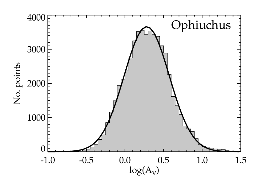
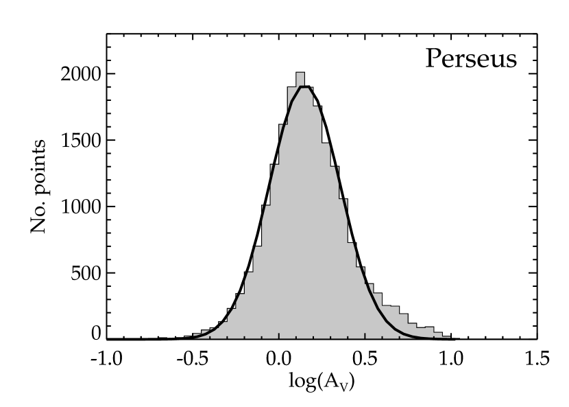
Figure 5: Histograms of extinction as derived from 2MASS in Ophiuchus (left) and Perseus (right) for the areas shown in figures 3 and 4 (filled histograms) overplotted with a log-normal fit to the data (thick black curve).

2.2 Extinction and Temperature Maps from IRAS

IRIS images (Miville-Deschênes & Lagache, 2005) of 60 and 100 $\mu$m flux density were obtained for the two regions. IRIS data offer excellent correction for the effects of zodiacal dust and striping in the unprocessed IRAS images and also provide improved gain and offset calibration over earlier releases (e.g. ISSA), which did not have an appropriate zero-point calibration. This can have serious consequences on the derived dust temperature and column density (Arce & Goodman, 1999a, b).

We used the method described in Schnee et al. (2005) (which is adaptation of the method used by Wood et al. 1994 and Arce & Goodman 1999a) to calculate the dust color temperature and column density from the IRIS 60 and 100 $\mu$m flux densities. The temperature is determined by the ratio of the 60 and 100 $\mu$m flux densities, assuming that the dust in a single beam is isothermal (the validity and implications of this assumption are discussed in detail in Schnee et al. 2005 and Schnee, Bethell, & Goodman 2006). Then the column density of dust can be derived from measured flux and the derived color temperature of the dust. The calculation of temperature and column density depends on the values of three parameters: two constants that determine the emissivity spectral index and the conversion from 100 $\mu$m optical depth to visual extinction. These parameters are solved for explicitly using the independent estimate of visual extinction we have from our 2MASS/NICER extinction maps (described in sect. 2.1).

The 2MASS/NICER extinction maps are used as a “model” of the extinction, and the three free parameters adjusted until the IRIS-implied column density best matches that of the “model”. The parameter values determined by this method are those that create a FIR-based extinction map that best matches the 2MASS/NICER extinction map on a statistical point-by-point basis, and is not a spatial match to features in the 2MASS/NICER extinction map.

Each cloud is considered separately, so the derived values of the three parameters are different for each cloud. We assume that the values of the three parameters are constant within each image, although this does not have to be the case. For instance, it is likely that areas of especially high or low column density do not share the same far-IR column-density to visual extinction conversion factor.

The IRAS-based extinction and temperature maps for Perseus and Ophiuchus are shown in figures 6 and 7 and their properties are given in table 4.

Table 4: IRAS Data

	Ophiuchus	Perseus
Pixel Size (′)	5	5
Effective Resolution (′)	5	5
Areal Coverage (degrees)	6.3$\times$6.4	7$\times$4.5

The IRAS-based extinction map of Ophiuchus shows a general similarity to the 2MASS-based extinction map. Notable differences, however, include an extension of moderate extinction to the northwest of L1688 and a regular series of high extinction peaks running west of L1689. Although there is some enhanced extinction northwest of L1688 in the 2MASS/NICER map, this difference is likely an example of how the IRAS-based extinction maps can be biased toward warmer dust, and possibly suggests warmer dust in that region due to external heating by the star $\rho$ Oph itself (Schnee et al., 2005). A notable feature in the temperature map is a heated ring, visible just to the north of L1688 and centered on the star B-star $\rho$-Oph.

Unlike in Ophiuchus, the IRAS-based extinction map of Perseus (figure 7, left panel) shows a vastly different morphology from the 2MASS/NICER extinction map (on more careful inspection, and by comparison with the dust color-temperature map (figure 7, right panel) the known dark cores in Perseus are visible however). This is because the column density as measured by IRAS is dominated by a  0.75^∘ warm shell, probably caused by emission from transiently heated small dust grains at the edge of an Hii region created by the B0 star HD 278942 (Ridge et al., 2005; Andersson et al., 2000).

Figure 6: Column density (left) and temperature (right) in Ophiuchus derived from IRAS. The contour indicates A_V of 3 mag. as in figure 3. NOTE TO EDITOR: THIS FIGURE SHOULD BE TYPESET FULL-PAGE, LANDSCAPE ORIENTATION

Figure 7: Column density (left) and temperature (right) in Perseus derived from IRAS. The contour indicates A_V of 3 mag. as in figure 4. NOTE TO EDITOR: THIS FIGURE SHOULD BE TYPESET FULL-PAGE, LANDSCAPE ORIENTATION

Histograms showing the distribution of extinctions and temperatures in the two regions are shown in figures 8 and 9. Detailed discussion of the histograms and a comparison of the histograms produced from IRAS and 2MASS/NICER appear in Schnee et al. (2005) and Goodman et al. (2006) respectively, but they are included here for completeness. Note that due to their differing resolution the histograms presented here are not directly comparable with those presented for the 2MASS/NICER extinction and CO data in sections 2.1 and 2.4.

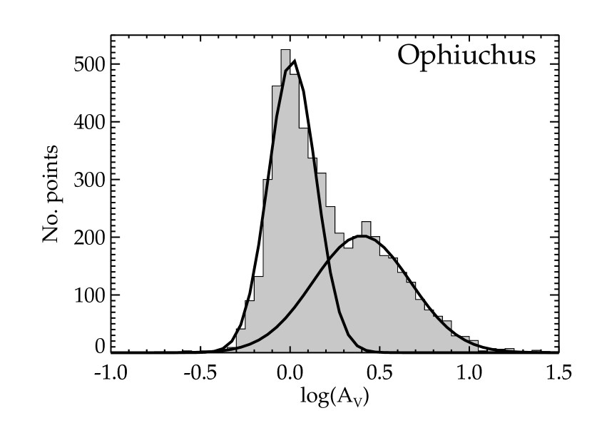
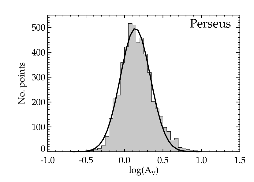
Figure 8: Histograms of extinction as derived from IRAS 60 and 100 $\mu$m emission in Ophiuchus (left) and Perseus (right) for the areas shown in figures 3 and 4 (filled histograms) overplotted with a log-normal fit to the data (thick black curves; in the case of Ophiuchus, a two component fit was used).

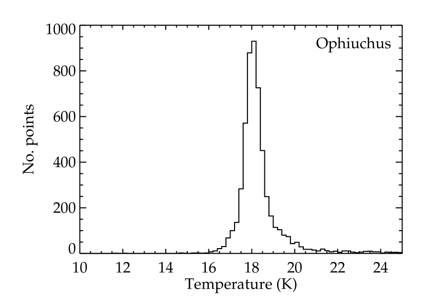
Figure 9: Histograms of temperature as derived from IRAS in Ophiuchus (left) and Perseus (right) for the areas shown in figures 3 and 4. Note that the relatively low resolution of these maps ($\sim 5^{\prime}$) means that we are not sensitive to the coldest densest regions within the clouds, and hence the average temperature is somewhat higher than the $\sim$10 K more typically associated with molecular clouds.

2.3 Atomic Hydrogen Maps from GBT

Maps of 21 cm HI emission over the Ophiuchus and Perseus clouds, covering 5 deg² and 20  deg² respectively, were obtained with the 100 m NRAO Green Bank Telescope (GBT) in West Virginia, USA over two observing runs in 2004 March and 2005 April. Both maps cover the densest cores in the regions as well as regions of substantially lower density, where HI could be stronger in emission due to the prevalence of atomic hydrogen, rather than molecular hydrogen. On-the-fly mapping and frequency switching with a 1 MHz throw were used together with a data dumping rate of twice the Nyquist sampling rate, i.e. 4 dumps as the telescope moves over a whole beam. The 12.5 MHz total bandwidth mode of the GBT Spectrometer was used with two spectral windows, one at 1420.4 MHz for HI, the other centered at 1666.4 MHz for the two OH lambda-doubling lines at 1667.4 MHz and 1666.4  MHz. Each spectral window has two linear polarizations, for a total of 4 IF inputs. With 16,384 lags, a 0.76 kHz channel width was achieved.

During reduction, frequency-switched data at both frequencies ($+/-$ frequency throw) were treated independently because of instrument baseline stability. The data were reduced using IDL routines written by G. Langston that are consistent in terms of calibration when checked with AIPS++ packages provided by NRAO. Conversion to antenna temperature was achieved through scaling by a noise tube input, and conversion to absolute flux levels was achieved through comparisons with observations of Mars. Calibrated data were regridded to 4^′ spacing in AIPS. The final data have an angular resolution of $\sim$9^′ FWHM, a spectral resolution of 0.32  km s^-1, and a typical 1-$\sigma$ rms noise of 0.15 K per channel. The properties of the HI maps are summarised in table 5. 3-D fits files can be viewed online at the COMPLETE website – the value of these data is in the spectral information and hence we do not show an integrated intensity map here. The angular resolution is comparable to the size of the dense structures in the two regions surveyed.

Table 5: HI Data

	Ophiuchus	Perseus
Pixel Size (′)	4	4
HPBW (′)	9	9
Areal Coverage (sq. degrees)	5	20
1$\sigma$ rms/channel (K)	0.15	0.15
Spectral Resolution ( km s-1)	0.32	0.32

The line profiles of HI in Ophiuchus reveal a strong and extensive HI Narrow Self-Absorption (HINSA; Li & Goldsmith, 2003) component, which is well correlated with molecular emission. This is consistent with previous pointed observations of the same region at a much lower resolution (Goodman & Heiles, 1994). Channel maps of HI emission between 8 to 11  km s^-1 suggest a possible association of HI gas in this velocity range with the heated ring seen in warm the IRAS temperature map.

The main component of HI emission toward the line of sight of Perseus is centered around 4 to 8  km s^-1, with the velocity of peak emission becoming redder toward the west of the region, as is seen in the molecular gas. The HI peaks, however, tend to be on the bluer side of the molecular gas by 1–2  km s^-1. For example, around dense core B1, the HI emission shows approximately a single Gaussian profile with peak velocity at 4.8  km s^-1, while ¹³CO peaks at $\sim$6.7  km s^-1 (figure 10).

Figure 10: Spectra of HI and ¹³CO at the position of the dense core B1. The molecular gas (as traced by the ¹³CO) has a peak velocity offset by $\sim$2  km s^-1 from the atomic gas. Both spectra are centered on the position 03^h33^m17$\fs$8 +31^∘07^m30^s (J2000).

The line-width of HI emission in Perseus is around 7–10  km s^-1 FWHM. Unlike other nearby regions, such as Taurus and Ophiuchus, the HINSA component is only seen toward a small portion of the dense clouds. This may be explained by viewing geometry and the different distances of the Perseus components. A minor, but very interesting component in our Perseus map is the presence of high velocity line wings in HI emission, extending from the main component all the way down to $-$50  km s^-1, where it peaks up again to possibly reflect HI emission from another galactic arm (figure 11). Although its origin is unclear at the moment, it is worth noting that it is probably too wide to be explained by a single low level HI emission component somewhere else in the galaxy.

Figure 11: Spectrum of HI emission at the position 03^h46^m21$\fs$6 +33^∘26^m48$\fs$5 (J2000), showing an extended line wing and second component, possibly from another Galactic arm.

2.4 Molecular Line Maps from FCRAO

Observations in the ¹²CO 1–0 (115.271 GHz) and ¹³CO 1–0 (110.201 GHz) transitions were carried out throughout the 2002–2005 observing seasons at the 14 m Five College Radio Astronomy Observatory (FCRAO) telescope in New Salem, MA, U.S.A. The SEQUOIA 32-element focal-plane array and an On-the-Fly mapping technique were used to make $10^{\prime}\times 10^{\prime}$ submaps. The dual-IF narrowband digital correlator enabled ¹²CO and ¹³CO to be observed simultaneously. The correlator was used in a mode that provided a total bandwidth of 25 MHz with 1024 channels in each IF, yielding an effective velocity resolution of 0.07  km s^-1. Data were taken during a wide range of weather qualities and system temperatures were generally between 500 and 1000 K at 115 GHz and 200 and 600 K at 110 GHz (single sideband). Due to its low elevation, system temperatures for Ophiuchus were consistently higher than for Perseus. Submaps with higher system temperatures were repeated to achieve uniform sensitivity where possible.

The submaps were obtained by scanning in the Right Ascension direction, and an off-source reference scan was obtained after every two or four rows, depending on weather and elevation. Off-positions were checked to be free of emission by making separate 10^′ OTF maps, with an off-position an additional 30^′ offset. Calibration was found via the chopper-wheel technique (Kutner & Ulich, 1981), yielding spectra with units of ${\rm{T}_{A}}^{*}$. Pointing was checked regularly and found to vary by less than 5^′′ rms.

Due to dewar rotation, the OTF data are not not evenly sampled, and so a convolution and regridding algorithm has to be applied to the data to obtain spectra on a regularly sampled grid. This process was carried out on the individual $10^{\prime}\times 10^{\prime}$ submaps using software provided by the observatory (Heyer et al., 2001). After subtraction of a linear baseline, each spectrum was convolved with nearby spectra onto a regular 23^′′ grid weighted by rms^-2, yielding a Nyquist-sampled map. The submaps were then combined into the final map using an IDL routine, and corrected for the main beam efficiency (0.5 and 0.45 at 110 and 115 GHz respectively). Due to the nature of the OTF technique, spectra in pixels near the edges of the map have a significantly higher rms noise. Hence an rms filter was applied to the combined map to blank pixels which had an rms noise of more than 3 times the mean rms noise for the entire map. Histograms, showing the range of rms noise in the final 3-dimensional data cubes are presented in figure 12.

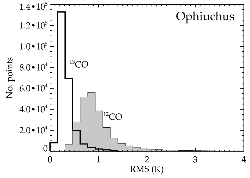
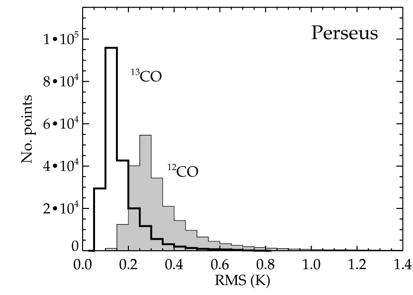
Figure 12: Histograms of rms noise per channel in the ¹²CO and ¹³CO maps of Ophiuchus (left) and Perseus (right).

The resolution, coverage, sampling and sensitivity of the resulting data cubes are summarised in table 6. Figure 13 shows average ¹²CO and ¹³CO spectra for Ophiuchus and Perseus, created by summing the spectra in all pixels where the ratio of peak antenna temperature to rms noise is greater than 3.

Table 6: CO Data

		Ophiuchus	Perseus
	Pixel Size (′′)	23	23
	Total number of spectra	244874	214316
	Areal Coverage (sq. degrees)	10.0	8.7
	HPBW (′′)	46	46
12CO	Mean RMS/channel (K)	0.98	0.35
	Min RMS/channel (K)	0.31	0.11
	Spectral Resolution ( km s-1)	0.064	0.064
	HPBW (′′)	44	44
13CO	Mean RMS/channel (K)	0.33	0.17
	Min RMS/channel (K)	0.10	0.06
	Spectral Resolution ( km s-1)	0.066	0.066

Figure 13: Average ¹²CO (thin lines) and ¹³CO (thick lines) spectra for Ophiuchus (left) and Perseus (right), created by summing the spectra in all pixels where the ratio of peak antenna temperature to rms noise is was greater than 3. The multi-component nature of Perseus is clearly visible, whilst Ophiuchus displays a more Gaussian-like profile.

Integrated intensity maps of ¹²CO and ¹³CO emission were made by summing over the range of velocities in which emission was seen. The integrated intensity maps of ¹³CO in Ophiuchus and Persus are shown in figures 14 and 15. The ¹²CO maps are not shown here but can be viewed online at the COMPLETE website.

Figure 14: Integrated intensity image of ¹³CO emission in Ophiuchus, overlaid with the positions of the dense cores detected in submillimeter continuum emission (red circles; see section 2.5). Symbol size is proportional to the mass of the core. The black contour indicates A_V=3 mag. from the 2MASS/NICER map, and the grey contour indicates A_V=15 mag., the implied threshold for dense core formation in Ophiuchus.

Figure 15: Integrated intensity image of ¹³CO emission in Perseus, overlaid with the positions of the dense cores detected in submillimeter continuum emission (red circles; see section 2.5). Symbol size is proportional to the mass of the core. The black contour indicates A_V=3 mag. from the 2MASS/NICER map, and the grey contour indicates A_V=6 mag., the implied threshold for dense core formation in Perseus.

Although extensive, the CO maps are more limited in areal coverage than the preceding datasets. For instance, the northeast filament and north west extension we see in the extinction map of Ophiuchus are not well sampled in CO emission. While the morphology generally follows that of the extinction map, a bright maxima north of the Oph A core within L1688 is quite prominent in the ¹³CO map of Ophiuchus. The average ¹²CO and ¹³CO spectra (figure 13, left panel) show an approximately Gaussian profile with a maximum width of $\sim$7  km s^-1. Table 7 gives the central velocity and FWHM obtained by fitting a Gaussian profile to the average spectra.

Table 7: Results of Gaussian fits to the average ¹²CO and ¹³CO lines in Ophiuchus.

	FWHM	VLSR
	km s-1	km s-1
12CO	2.77	3.38
13CO	2.38	3.38

The morphology of the integrated CO intensity in Perseus is again similar to that of the extinction, but due to their $\sim$4 times better linear spatial resolution over the extinction map, the ¹²CO and ¹³CO maps reveal complex substructure within the clumps we see in extinction. The CO emission shows components at multiple velocities, and a steep velocity gradient across the cloud complex, with a difference of almost 10  km s^-1 over the $\sim$30 pc east-west extent of the complex. This is the main cause of the wide line-widths ($\sim$ 15  km s^-1) and non-Gaussian profiles exhibited by the average ¹²CO and ¹³CO spectra shown in figure 13, and suggests that the Perseus complex is much more dynamic than Ophiuchus.

Histograms of the ¹²CO and ¹³CO integrated intensity are shown in figure 16. Unlike the 2MASS/NICER extinction maps, the distribution of CO intensities does not follow a log-normal distribution. In particular there is a significant low-intensity tail to the distribution. In Perseus, the distribution also appears somewhat truncated on the high-intensity side. This is likely a result of a combination of chemical effects (e.g. freeze-out) and high optical-depth of both ¹²CO and ¹³CO at higher column densities. The warmer temperatures (as traced by the IRAS temperature map) in the densest regions of Ophiuchus may prevent CO freezing out there.

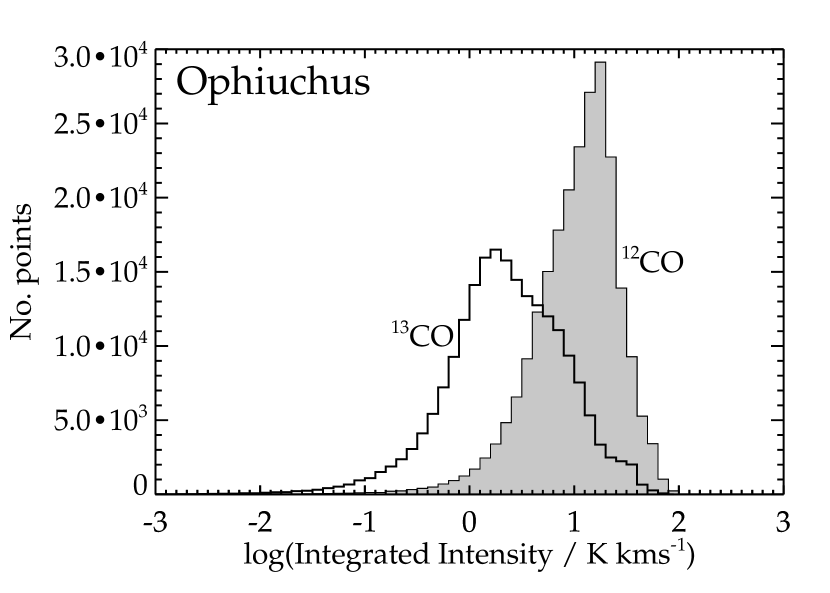
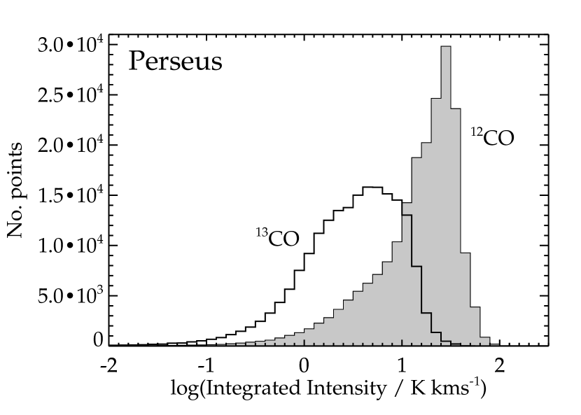
Figure 16: Histograms of ¹²CO and ¹³CO integrated intensity for Ophiuchus (left) and Perseus (right).

2.5 Thermal Dust Emission Maps from JCMT

Submillimeter continuum data at 850 $\mu$m of the Ophiuchus and Perseus molecular clouds were obtained using the Submillimetre Common User Bolometer Array (SCUBA) on the 15 m James Clerk Maxwell Telescope (JCMT) on Mauna Kea, HI, U.S.A. The data presented here are a combination of our own observations ($\sim$5.6 deg² of Ophiuchus and $\sim$1.3 deg² of Perseus) with publicly available archival data for a total of $\sim$5.8 deg² of Ophiuchus and $\sim$3.5 deg² of Perseus.

All raw data were first flat-fielded and extinction corrected using the standard SCUBA software (Holland et al., 1999). The data were then converted into images by applying the matrix inversion technique of Johnstone et al. (2000) with a pixel size of 6″. Although the maps have an intrinsic beamsize of 14″, their effective beamsize is 19.9″ because each was convolved with a $\sigma$ = 6″ Gaussian to reduce pixel noise. Structure on scales several times larger than the chop throw ($>$120″) may be an artifact of image reconstruction (independent of the technique; see Johnstone et al. 2000). Large-scale artifacts were removed by subtracting a convolved version of the original map (made with a Gaussian of $\sigma$ = 90″) from each map. To minimize the occurrence of artificial negative “bowls” around bright sources resulting from this technique, all pixels with values $>|5|$ times the mean noise were set to specifically +5 or -5 times the mean noise prior to convolution. Since each map was constructed from data obtained under a variety of weather conditions, the noise across each map is not uniform. The noise variation across each map, however, is typically only a factor of a few. The mean and rms standard deviation are $\sim$40 and 20 mJy beam^-1 respectively in Ophiuchus and $\sim$8 and $\sim$7 mJy beam^-1 respectively in Perseus. Due to their size, it is not possible to display the maps clearly in this work, and again we refer the reader to the COMPLETE website where fits files are publically available. The properties of the maps are summarised in table 8.

Table 8: SCUBA 850$\mu$m Continuum Data

	Ophiuchus	Perseus
Pixel Size (′′)	6	6
Effective Resolution (′′)	19.9	19.9
Areal Coverage (sq. degrees)	5.8	3.5
Mean RMS noise (mJy beam-1)	40 (20)	8 (7)

Detailed analyses and images of the submillimeter maps are presented in Johnstone, Di Francesco, & Kirk (2004) for Ophiuchus and Kirk, Johnstone, & Di Francesco (2006) for Perseus, or can be viewed online at the COMPLETE website so are not repeated here. The positions of the dense clumps detected in the submillimeter are shown as red circles in figures 14 and 15.

Of particular interest in the Ophiuchus map is the lack of any submillimeter emission northwest of L1688, which was well covered with SCUBA as a result of the IRAS-based extinction map showing possible moderate extinction in that direction. This lack of detection is likely due to especially low sensitivity to extended, diffuse structures that may inhabit that location (see Johnstone et al. 2004). Also, as has been discussed in Johnstone et al. (2004), there appears to be threshold of column-density (extinction) below which no dense cores are found. In the case of Ophiuchus this threshold is at an A_V of $\sim$15 mag, as indicated by the grey contour in figure 14.

Like in Ophiuchus, all of the dense submillimeter clumps in Perseus are found to lie within the larger high-extinction regions, but the threshold of $\sim$5–7 A_V is somewhat lower than in Ophiuchus. This difference in thresholds cannot be attributed to the different sensitivities of the two submillimeter maps – this is discussed further in Kirk et al. (2006). A similar threshold has also been reported by Hatchell et al. (2005) and Enoch et al. (2006).

3 Summary

We have presented maps of the gas and dust in the Ophiuchus and Perseus star-forming regions, obtained using a range of different techniques, and providing information on the star-forming material on scales of  0.1-10pc. These observations complement the observations made as part of the Spitzer Space Telescope “From Molecular Cores to Planet Forming Disks” Legacy Program, which provides a catalogue of the young stars.

Some highlights of the data are:

• The apparent morphology and distribution of star-forming material varies significantly between different column-density tracers, with the near-infrared extinction method providing the closest match to the log-normal distribution of material predicted by numerical simulations.

• CO emission in Ophiuchus shows approximately Gaussian line shapes, while Perseus appears much more dynamic, with multiply peaked, wide, non-Gaussian lines.

• There appears to be an extinction threshold below which dense sub-mm cores are not detected. This threshold varies from region to region (A${}_{V}\sim$15 in Ophiuchus and $\sim$5-7 in Perseus).

• HI emission in Perseus shows an extremely high-velocity line wing, possibly reflecting emission from another Galactic arm.

All of the data sets presented here are publically available from the COMPLETE website.

References

- Andersson et al. (2000) Andersson, B. G., Wannier, P. G., Moriarty-Schieven, G. H., & Bakker, E. J. 2000, AJ, 119, 1325
- Arce & Goodman (1999a) Arce, H. G., & Goodman, A. A. 1999a, ApJ, 517, 264
- Arce & Goodman (1999b) —. 1999b, ApJ, 512, L135
- de Geus et al. (1989) de Geus, E. J., de Zeeuw, P. T., & Lub, J. 1989, A&A, 216, 44
- Enoch et al. (2006) Enoch, M., Young, K., Glenn, G., Evans, N., Golwala, S., Sargent, A., Harvey, P., Aguirre, A., Goldin, A., Haig, D., Lange, A., Laurent, G., Maloney, P., Mauskopf, P., Rossinot, P., & Sayers, J. 2006, ApJ, accepted (astro-ph/0510202)
- Evans et al. (2003) Evans, N. J., Allen, L. E., Blake, G. A., Boogert, A. C. A., Bourke, T., Harvey, P. M., Kessler, J. E., Koerner, D. W., Lee, C. W., Mundy, L. G., Myers, P. C., Padgett, D. L., Pontoppidan, K., Sargent, A. I., Stapelfeldt, K. R., van Dishoeck, E. F., Young, C. H., & Young, K. E. 2003, PASP, 115, 965
- Goodman & Heiles (1994) Goodman, A. A., & Heiles, C. 1994, ApJ, 424, 208
- Goodman et al. (2006) Goodman, A. A., Schnee, S. L., & Ridge, N. A. 2006, in prep.
- Hatchell et al. (2005) Hatchell, J., Richer, J. S., Fuller, G. A., Qualtrough, C. J., Ladd, E. F., & Chandler, C. J. 2005, A&A, 440, 151
- Heyer et al. (2001) Heyer, M. H., Narayanan, G., & Brewer, M. K. 2001, On the Fly Mapping at the FCRAO 14m Telescope, FCRAO, http://www.astro.umass.edu/fcrao/library/manuals/otfmanual.html
- Holland et al. (1999) Holland, W. S., Robson, E. I., Gear, W. K., Cunningham, C. R., Lightfoot, J. F., Jenness, T., Ivison, R. J., Stevens, J. A., Ade, P. A. R., Griffin, M. J., Duncan, W. D., Murphy, J. A., & Naylor, D. A. 1999, MNRAS, 303, 659
- Indebetouw et al. (2005) Indebetouw, R., Mathis, J. S., Babler, B. L., Meade, M. R., Watson, C., Whitney, B. A., Wolff, M. J., Wolfire, M. G., Cohen, M., Bania, T. M., Benjamin, R. A., Clemens, D. P., Dickey, J. M., Jackson, J. M., Kobulnicky, H. A., Marston, A. P., Mercer, E. P., Stauffer, J. R., Stolovy, S. R., & Churchwell, E. 2005, ApJ, 619, 931
- Johnstone et al. (2004) Johnstone, D., Di Francesco, J., & Kirk, H. 2004, ApJ, 611, L45
- Johnstone et al. (2000) Johnstone, D., Wilson, C. D., Moriarty-Schieven, G., Giannakopoulou-Creighton, J., & Gregersen, E. 2000, ApJS, 131, 505
- Kirk et al. (2006) Kirk, H., Johnstone, D., & Di Francesco, J. 2006, ApJ, submitted
- Kutner & Ulich (1981) Kutner, M. L., & Ulich, B. L. 1981, ApJ, 250, 341
- Lada (1992) Lada, E. A. 1992, ApJ, 393, L25
- Li & Goldsmith (2003) Li, D., & Goldsmith, P. F. 2003, ApJ, 585, 823
- Lombardi & Alves (2001) Lombardi, M., & Alves, J. 2001, A&A, 377, 1023
- Lombardi & Alves (2006) —. 2006, in prep.
- Lombardi et al. (2006) Lombardi, M., Alves, J., & Lada, C. 2006, A&A, submitted
- Lombardi & Schneider (2001) Lombardi, M., & Schneider, P. 2001, A&A, 373, 359
- Miville-Deschênes & Lagache (2005) Miville-Deschênes, M.-A., & Lagache, G. 2005, ApJS, 157, 302
- Ostriker et al. (2001) Ostriker, E. C., Stone, J. M., & Gammie, C. F. 2001, ApJ, 546, 980
- Ridge et al. (2006) Ridge, N. A., Schnee, S. L., Goodman, A. A., & Borkin, M. A. 2006, in prep.
- Ridge et al. (2005) Ridge, N. A., Schnee, S. L., Goodman, A. A., & Foster, J. B. 2005, ApJ, submitted
- Rieke & Lebofsky (1985) Rieke, G. H., & Lebofsky, M. J. 1985, ApJ, 288, 618
- Schnee et al. (2006) Schnee, S. L., Bethell, T., & Goodman, A. A. 2006, ApJ, submitted
- Schnee et al. (2005) Schnee, S. L., Ridge, N. A., Goodman, A. A., & Li, J. G. 2005, ApJ, 634, 442
- Walawender et al. (2005) Walawender, J., Bally, J., Kirk, H., & Johnstone, D. 2005, AJ, 130, 1795
- Wood et al. (1994) Wood, D. O. S., Myers, P. C., & Daugherty, D. A. 1994, ApJS, 95, 457