Accelerated Cosmological Models in
Modified Gravity
tested by distant Supernovae SNIa data.

Abstract

Recent type Ia supernova measurements and other astronomical observations suggest that our universe is, at the present epoch, in an accelerating phase of evolution. While a dark energy of unknown form and origin was usually proposed as the most feasible mechanism for the acceleration, there appeared some generalizations of Einstein equations which could mimic dark energy. In this work we investigate observational constraints on a modified Friedmann equation obtained from the generalized Lagrangian ${\cal L}\propto R^{n}$ minimally coupled with matter via the Palatini first-order formalism. We mainly concentrate on such restrictions of model parameters which can be derived from distant supernovae and baryon oscillation tests. We obtain confidence levels for two parameters ($n$, $\Omega_{m,0}$) and find, from combined analysis, that the preferred value of $\Omega_{m,0}$ equals $0.3$. For deeper statistical analysis and for comparison of our model with predictions of the $\Lambda$CDM concordance model one applies Akaike and Bayesian information criteria of model selection. Finally, we conclude that the Friedmann-Robertson-Walker (FRW) model merged with a first-order non-linear gravity survives SNIa and baryon oscillation tests.

I Introduction

The recent observations of type Ia distant supernovae indicate that our Universe is currently accelerating Riess:1998cb ; Perlmutter:1998np . There are different proposals for explaining this phenomenon. Some of them are based on assumptions of standard cosmological models, which utilize FRW metric. Thus possible explanations include: cosmological constant $\Lambda$ Weinberg:1989 ; Carroll:1992 , a decaying vacuum energy density Vishwakarma:2001 , an evolving scalar field or quintessence models Ratra:1998 , a phantom energy (expressed in terms of the barotropic equation of state violating the weak energy condition) Caldwell:1999ew ; Dabrowski:2003 , dark energy in the form of Chaplygin gas Kamenshchik:2001cp , etc.. All these conceptions propose some kind of new matter of unknown origin which violate the strong energy condition. The Universe is currently accelerating due to the presence of these dark energy components.

On the other hand, there are alternative ideas of explanation, in which instead of dark energy some modifications of Friedmann’s equation are proposed at the very beginning. In these approaches some effects arising from new physics like brane cosmologies, quantum effects, anisotropy effects etc. can mimic dark energy by a modification of Friedmann equation. Freese & Lewis Freese:2002sq have shown that contributions of type $\rho^{n}$ to Friedmann’s equation $3H^{2}=\rho_{eff}$, where $\rho$ is the energy density and $n$ a constant, may describe such situations phenomenologically. These models (by their authors called the Cardassian models) give rise to acceleration, although the universe is flat and contains the usual matter and radiation without any dark energy components. In the authors’ opinion Freese:2002sq , what is still lacking is a fundamental theory (like general relativity) from which these models can be derived after postulating Robertson Walker (R-W) symmetry. We argue that a possible candidate for such a fundamental theory can be provided by non-linear gravity theories (for a recent review see e.g. NO and references therein) and, particularly, the so-called $f(R)$- theories Cap . It is worth pointing out that if one imposes the energy-momentum conservation condition then matter density is parametrized by the scale factor (in a case of R-W symmetry), and Cardassian term $\rho^{n}$ in the Friedmann equation will be reproduced.

There are different theoretical attempts to modify gravity in order to achieve an accelerating cosmic expansion at the present epoch. Already in the paper by Carroll et al. Carroll04 , one can find interesting modifications of the Einstein-Hilbert action with Lagrangian density ${\cal L}\propto R+f(R,P,Q)$. Those authors have shown that in the generic case cosmological models admit, at late time, a de Sitter solution, which is unfortunately unstable. Moreover, Carroll et al. have demonstrated the existence of an interesting set of attractors, which seem to be important in the context of the dark energy problem.

The main goal of the present paper is to set up observational constraints on parameters of cosmological models inspired by non-linear gravity. The possibility of explaning cosmic acceleration in terms of nonlinear generalization of the Einstein equation has been previously addressed in XY ; XX . However, these authors have not confronted their models with observational data. This problem has been tackled in yy , where nonlinear power law lagrangians were compared with SNIa data and X ray gas mass fraction as well (see also mota for a more general class of lagrangians). Here, we use samples of supernovae Ia Riess:2004nr ; Astier:2005 together with the baryon oscillation test Eisenstein:2005 for stringent and deeper constraint on model parameters. We check to which extent the predictions of our model are consistent with the current observational data.

Severe constraints on the particular modifications of gravity considered in this paper have been already proposed Cap ; yy ; mota ; Severe . On the other hand, in the article by Clifton and Barrow Clifton05 , strong constraints coming from nucleosynthesis of light elements have been found within a higher-order gravity. Therefore, it is possible that our model (although a first-order), which fits SNIa data well can be ruled out by nucleosynthesis arguments.

Assuming FRW dynamics in which dark energy is present, the basic equation determining a cosmic evolution has the form of a generalized Friedmann equation

$$H^{2}=\frac{\rho_{\mathrm{eff}}}{3}-\frac{k}{a^{2}}\ ,$$ (1)

where $\rho_{\mathrm{eff}}(a)$ stands for the effective energy density of several “fluids”, parametrized by the scale factor $a$, while $k=\pm 1,0$ denotes the spatial curvature index. One can reformulate (1) in terms of density parameters $\Omega_{i}$ as

$$\frac{H^{2}}{H_{0}^{2}}=\Omega_{\mathrm{eff}}(z)+\Omega_{k,0}(1+z)^{2}\ ,$$ (2)

where $\frac{a}{a_{0}}=\frac{1}{1+z}$, $\Omega_{\mathrm{eff}}(z)=\Omega_{m,0}(1+z)^{3}+\Omega_{X,0}f(z)$ and $\Omega_{m,0}$ is the density parameter for the (baryonic and dark) matter, scaling like $a^{-3}$, while $f(z)$ describes the dark energy $X$. For $a=a_{0}$ (the present value of the scale factor which we further on normalize to unity), one obtains the constraint $\Omega_{\mathrm{eff,0}}+\Omega_{k,0}=1$.

We can certainly assume that the energy density ($i=m,X$) satisfies the conservation condition

$$\dot{\rho}_{i}=-3H(\rho_{i}+p_{i})$$ (3)

for each component of the fluid, so that $\rho_{\mathrm{eff}}=\Sigma\rho_{i}$. Then from  (2) one gets the constraint relation $\Sigma_{i}\Omega_{i,0}+\Omega_{k,0}=1$ for the present values ($z=0$) of the density parameters.

All approaches mentioned above lead toward a description of dark energy in the framework of standard FRW cosmology. It will be demonstrated, in the next Section, that all cosmological models of the first-order non-linear gravity which satisfy R-W symmetry, can also be reduced to the familiar form (2). Therefore, the effects of nonlinear gravity can mimic dynamical effects of dark energy.

II FRW cosmology and first-order non-linear gravity

For the cosmological applications one chooses the Friedmann-Robertson-Walker metric, which (in spherical coordinates) takes the standard form:

$$g=-dt^{2}+a^{2}(t)\Big{[}{1\over{1-kr^{2}}}dr^{2}+r^{2}\Big{(}d\theta^{2}+\sin^{2}(\theta)d\varphi^{2}\Big{)}\Big{]}\ .$$ (4)

As before, $a(t)$ denotes the scale factor and $k$ the spatial curvature ($k=0,1,-1$). Another main ingredient of all cosmological models is a perfect fluid stress-energy tensor, expressed by

$$T_{\mu\nu}=\left(\begin{array}[]{clcr}\rho&0&0&0\\ 0&\frac{pa^{2}(t)}{1-kr^{2}}&0&0\\ 0&0&pa^{2}(t)r^{2}&0\\ 0&0&0&pa^{2}(t)r^{2}\sin^{2}(\theta)\end{array}\right)\ .$$ (5)

One requires the standard relations between the pressure $p$, the matter density $\rho$, the equation of state parameter $w$ and the expansion factor $a(t)$, namely

$$p=w\rho\quad,\quad\rho=\eta a^{-3(1+w)},\quad,\quad\eta=\mathrm{const}.$$ (6)

Let us consider the action functional

$$A=A_{\mathrm{grav}}+A_{\mathrm{mat}}=\int(\sqrt{\det g}f(R)+2\kappa L_{\mathrm{mat}}(\Psi))d^{4}x$$ (7)

within the first order Palatini formalism XX . In fact, from now on we shall assume the simplest power law gravitational Lagrangian of the form

$$f(R)\sqrt{g}=\frac{\beta}{2-n}R^{n}\sqrt{g}\qquad(\beta\neq 0;\;n\in{I\kern-3.6ptR};\;n\neq 0,2)\ ,$$

where one fixes the constant $\beta$ to be positive (it has the same dimension as $R^{1-n}$). We want to point out that our model is singular for $n=2$. As shown in XX , such models are exactly solvable for the matter stress-energy tensor representing a single perfect fluid of a kind $w$ (cf. (6)). Their confrontation with experimental data has been performed, for a dust filled universe, in yy . Here we attempt to continue the analysis with newly available Astier SNIa samples and new baryon oscillation tests. These allow us to strengthen the admissible constraints on model parameters. Moreover, we extend our research to a matter stress-energy tensor containing two components, both with $p=w\rho$: a perfect fluid $w=\mathrm{const}\neq\frac{1}{3}$ and a radiation $w=\frac{1}{3}$. It turns out that the presence of the radiation term crucially changes the dynamics of our model at the early stage of its evolution. In addition, as to be demonstrated in Section III, although one cannot obtain better constraints from SNIa data, the combined analysis of SNIa and baryon oscillations offers a new possibility for a deeper determination of model parameters.

Following a method developed in XX , the Hubble parameter for our model can be calculated to be:

$$H^{2}=\frac{2n}{3(3w-1)[3w(n-1)+(n-3)]}\left[\frac{\kappa(1-3w)\eta_{w}}{\beta}\right]^{\frac{1}{n}}\,a^{-\frac{3(1+w)}{n}}+$$

$$+\frac{4n(2-n)\kappa\eta_{rad}}{3\beta[3w(n-1)+(n-3)]^{2}}\left[\frac{\kappa(1-3w)\eta_{w}}{\beta}\right]^{\frac{1-n}{n}}\,a^{-\frac{n+3+3w(1-n)}{n}}-\frac{k}{a^{2}}\,\left[\frac{2n}{3w(n-1)+(n-3)}\right]^{2}\ .$$ (8)

(Since radiation is already included in (8), one has to assume $w\neq{1\over 3}$.)

It is worth pointing out that the deceleration parameter, in the case $k=\eta_{rad}=0$, equals to (see XX ):

$$q(n,w)=\frac{3(1+w)-2n}{2n}=-1+\frac{3(1+w)}{2n}\ .$$ (9)

Thus, the effective equation of state parameter $w_{eff}$ is

$$w_{eff}=-1+{1+w\over n}\ .$$ (10)

Let us observe that, in the case $\eta_{rad}\neq 0$, $w<\frac{1}{3}$, the same values of $q(n,w)$ and $w_{eff}$ can also be achieved as asymptotic values $a\mapsto\infty$. In the early universe, when the scale factor goes to the initial singularity, the radiation term, in (8) scaling like $a^{-(1+\frac{3}{n})}$, will dominate over the dust term (scaling like $a^{-\frac{3}{n}}$). More precisely, if $n<0$ or $n>2$, then the negative radiation term cannot dominate over the matter, so that instead of the initial singularity we obtain a bounce. On the other hand, if $a$ goes to infinity, the radiation becomes negligible versus to the matter.

In our further analysis we restrict ourselves to the case $w=k=0$ i.e., more precisely, to the spatially flat universe filled with dust and radiation. Thus (8), (remarking once more that all $\eta$’s are positive constants) becomes

$$H^{2}=\frac{2n}{3(3-n)}\left[\frac{\eta_{dust}\kappa}{\beta}\right]^{1\over n}a^{-\frac{3}{n}}\,+\frac{4n(2-n)\kappa\eta_{rad}}{3\beta(n-3)^{2}}\left[\frac{\eta_{dust}\kappa}{\beta}\right]^{1-n\over n}a^{-\frac{n+3}{n}}-\frac{4kn^{2}}{(n-3)^{2}}\,a^{-2}\ .$$ (11)

One should immediately note that this expression, representing the squared Hubble parameter, reproduces in the case $n=\beta=1$ – as expected – the standard Friedmann equation. We would like to emphasize also that (11) becomes singular at $n=3$.

It is convenient to rewrite relation (11) is such a way that all coefficients are dimensionless (density parameters). Then, the effects of the matter scaling like $a^{-3(1+w)}$, and the radiation scaling like $a^{-4}$, can be separated from the effects of the nonlinear generalization of Einstein gravity ($n\neq 1$):

$$\left(\frac{H}{H_{0}}\right)^{2}=\Omega_{m,0}(1+z)^{3}\frac{2n}{\left(3-n\right)}\Omega_{nonl,0}(1+z)^{\frac{3\left(1-n\right)}{n}}+$$

$$+\Omega_{r,0}(1+z)^{4}\frac{4n\left(2-n\right)}{\left(n-3\right)^{2}}\Omega_{nonl,0}(1+z)^{\frac{3\left(1-n\right)}{n}}\ .$$ (12)

Here: $\Omega_{m,0}=\frac{\eta_{dust}\kappa}{3H^{2}_{0}}$, $\Omega_{r,0}=\frac{\eta_{rad}\kappa}{3H^{2}_{0}}$, $\Omega_{nonl,0}=\left(\frac{\eta_{dust}\kappa}{\beta}\right)^{\frac{1-n}{n}}$ while $H_{0}$ denotes the present-day value of the Hubble function. Let us observe that $\Omega_{nonl,0}$ can be determined also from the constraint $H(z=0)=H_{0}$, which easily reduces to:

$$\Omega_{nonl,0}=\left(\frac{2n}{\left(3-n\right)}\Omega_{m,0}+\frac{4n\left(2-n\right)}{\left(n-3\right)^{2}}\Omega_{r,0}\right)^{-1}\ .$$

The relation (12) has the form of Friedmann’s first integral. Therefore, the dynamics of the model can be naturally rewritten in terms of a 2D dynamical system of Newtonian type. Its Hamiltonian is:

$$\mathcal{H}\equiv\frac{1}{2}\dot{a}^{2}+V(a)=0\ ,$$ (13)

while the corresponding equations of motion are:

$$\dot{a} =y\ ,$$

$$\dot{y} =-\frac{\partial V}{\partial a}\ .$$ (14)

The overdot differentiats now with respect to the rescaled time variable $\tau$, so that $dt=|H_{0}|d\tau$, while $V(a)$ is a potential function for the scale factor $a$ expressed in units of its present value $a_{0}=1$. If $H^{2}=f(a)$, then the potential function is given by the general formula

$$V(a)=-\frac{1}{2}f(a)a^{2}\ .$$ (15)

For example, the potential function for our model writes as ($a_{0}=1$):

$$V(a)=-\frac{1}{2}\left[\frac{2n}{3-n}\Omega_{m,0}\,a^{-1}+\frac{4n\left(2-n\right)}{\left(n-3\right)^{2}}\Omega_{r,0}\,a^{-2}\right]\Omega_{nonl,0}\,a^{\frac{3}{n}\left(1-n\right)}\ .$$ (16)

Recently, in Carloni et al car , the cosmological dynamics of $R^{n}$ gravity has been treated in a different phase space with the use of qualitative methods for dynamical systems.

The phase portraits for the $\Lambda$CDM model versus our model with fitted values of $n,\Omega_{m,0}$ parameters (see the next Section) are illustrated on Figures 1 and 2. Both models are topologically inequivalent: the phase portrait of $\Lambda$CDM has a structurally stable saddle critical point, while with nonlinear gravity one obtains a center. As well-known, the critical point of a center type is structurally unstable and all trajectories around this point represent the models, which oscillate without initial and final singularities.

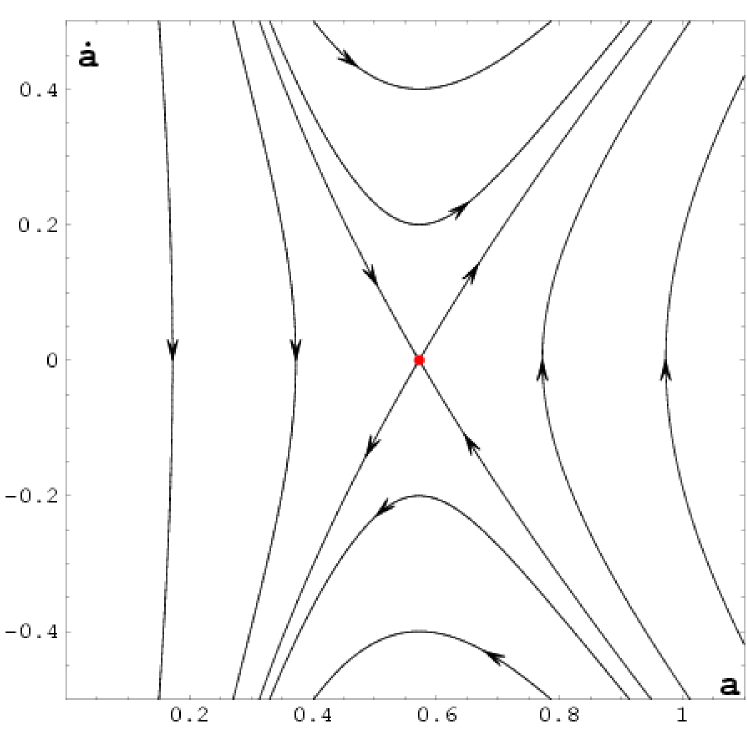
Figure 1: The phase portrait for the $\Lambda$CDM model. There is a single critical saddle-point on the $a$-axis. It represents the static Einstein universe. The trajectory of flat $k=0$ model divides all remaining ones into closed (inside) and open (outside) models.

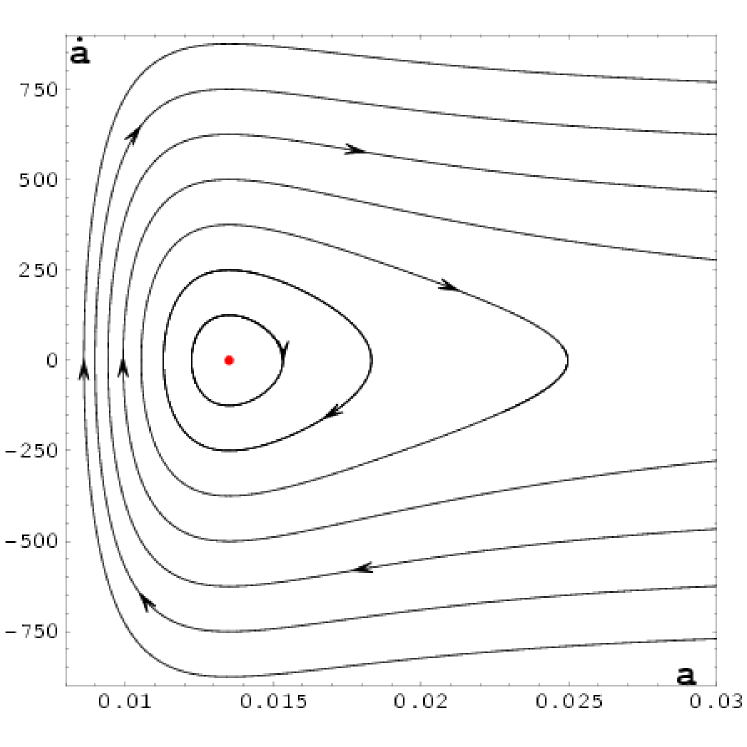
Figure 2: The phase portrait for nonlinear gravity with ${\cal L}\propto R^{n}$, $n=2.6$ (from estimation). There is a single critical point on the $a$-axis - a center; $a=a_{crit}=\frac{8n(n-2)}{(n-3)^{2}}\left(\frac{\Omega_{r,0}}{\Omega_{m,0}}\right)$. The trajectories of the system lie in the physical region $\{a:a>\frac{a_{crit}}{2}\}$ and represent bouncing evolution. In this scenario, instead of the big bang singularity of the $\Lambda$CDM model, one has a bounce $a=a_{min}$, $\ddot{a}>0$. It lies in a neighborhood of the minimum of the potential function. During the bounce phase, the universe is still accelerating. Note that if radiation effects vanish, there is no static critical point on the $a$-axis (formally $a_{crit}=0$ is allowed for $n>3$).

It is interesting that (12) after a time reparametrization following the rule: $d\eta=(1+z)^{\frac{3\left(1-n\right)}{2}}d\tau$ is equivalent to the standard cosmological model with matter and radiation, with rescaled values of the corresponding density parameters $\Omega_{m,0}$ and $\Omega_{r,0}$.

The geometry of the potential function offers the possibility to investigate the remaining models. On can simply establish some general relation between the geometry of the potential function and critical points of the Newtonian systems. In any case, the critical points lie on the $a$-axis, i.e. they represent the static solution $y_{0}=0,\ a=a_{0}$ so that $\left(\frac{\partial V}{\partial a}\right)_{a_{0}}=0$. If $(a_{0},0)$ is a strict local maximum of $V(a)$, it is of the saddle type. If $(a_{0},0)$ is a strict local minimum of the analytical function $V(a)$, it is a centre. If $(a_{0},0)$ is a horizontal inflection point of the $V(a)$, it is a cusp.

From the fitting procedure we obtain $n>2$, so the second term in the potential function is negative (in contrast to the first term which is positive). Because the negative radiation term in (16) can not dominate the first one ($V\leq 0$), there is the characteristic bounce behavior rather than the initial singularity in the $\Lambda$CDM model. Moreover, during the bouncing phase the universe is accelerating, while for late times it becomes matter dominated and decelerates.

III Distant supernovae as cosmological test

Type Ia distant supernova surveys suggest that the present Universe is accelerating Riess:1998cb ; Perlmutter:1998np . Every year new SNIa enlarge the available data by more distant objects and lower systematics errors. Riess et al. Riess:2004nr have compiled samples which become the standard data sets of SNIa. One of them, the restricted “Gold” sample of 157 SNIa, is used in our analysis. Recently Astier et al. Astier:2005 have compiled a new sample of supernovae, based on 71 high redshifted SNIa discovered during the first year of Supernovae Legacy Survey. This latest sample of 115 supernovae is used as our basic sample.

For distant SNIa one can directly observe their apparent magnitude $m$ and redshift $z$. Because the absolute magnitude $M$ is related to the absolute luminosity $L$, the relation between luminosity distance $d_{L}$, the observed magnitude $m$ and the absolute magnitude $M$ has the following form

$$m-M=5\log_{10}d_{L}+25\ .$$ (17)

It is convenient to use the dimensionless parameter $D_{L}$

$$D_{L}=H_{0}d_{L}$$ (18)

instead of $d_{L}$. Then  (17) can be replaced by

$$\mu\equiv m-M=5\log_{10}D_{L}+\mathcal{M}\ ,$$ (19)

where

$$\mathcal{M}=-5\log_{10}H_{0}+25\ .$$ (20)

We know the absolute magnitude of SNIa from its light curve. The luminosity distance of supernovae is a given function of the redshift:

$$d_{L}(z)=(1+z)\frac{c}{H_{0}}\frac{1}{\sqrt{|\Omega_{k,0}|}}\mathcal{F}\left(H_{0}\sqrt{|\Omega_{k,0}|}\int_{0}^{z}\frac{dz^{\prime}}{H(z^{\prime})}\right)\ ,$$ (21)

where $\Omega_{k,0}=-\frac{k}{H_{0}^{2}}$ and

$$\mathcal{F}(x) =\sinh(x)\qquad \qquad k<0\ ,$$ for

$$\mathcal{F}(x) =x\qquad \qquad k=0\ ,$$ for (22)

$$\mathcal{F}(x) =\sin(x)\qquad \qquad k>0\ .$$ for

Substituting (21) back into equations (17) and (19) provides us with an effective tool (Hubble diagram) to test cosmological models and to constrain their parameters. Assuming that supernovae measurements come with uncorrelated Gaussian errors, one can determine the likelihood function $\mathcal{L}$ from chi-square statistic $\mathcal{L}\propto\exp(-\chi^{2}/2)$, where

$$\chi^{2}=\sum_{i}\frac{(\mu_{i}^{\mathrm{theor}}-\mu_{i}^{\mathrm{obs}})^{2}}{\sigma_{i}^{2}}\ .$$ (23)

The Probability Density Function (PDF in short) of cosmological parameters Riess:1998cb can be derived from Bayes’ theorem. Therefore, one can estimate model parameters by using a minimization procedure. It is based on the likelihood function as well as on the best fit method minimizing $\chi^{2}$.

For statistical analysis we have restricted the parameter $\Omega_{m,0}$ to the interval $[0,1]$ and $n$ to $[-10.0,10.0]$ (except $n=0$ and additionally $n=3$ for $w=0$). Moreover, because of the singularity at $n=3,w=0$ (see eq. (12)) we have separated the cases $n>3$ and $n<3$ for $w=0$ in our analysis. Please note that $\Omega_{nonl,0}$ is obtained from the constraint $H(z=0)=H_{0}$.

In Figure 3 we present residual plots of redshift-magnitude relations (Hubble diagram) between the Einstein-de Sitter model (represented by zero line) and our best fitted model — upper curve — and $\Lambda$CDM model — middle curve. One can observe systematic deviations between these models at higher redshifts. The non-linear gravity model predicts that high redshifted supernovae should be fainter than those predicted by the $\Lambda$CDM model.

Figure 3: Residuals (in mag) between the Einstein-de Sitter model (zero line), the flat $\Lambda$CDM model (middle curve) and the non-linear gravity model (upper curve). Results obtained with the Astier (left panel) and the Riess (right panel) samples.

Figure 4: PDF obtained with the Astier sample for the parameters $\Omega_{m,0}$ and $n$, marginalised over the rest of parameters. Non-linear gravity model ($w=0$, $n<3$).

The results of two fitting procedures performed on Riess and Astier samples with different prior assumptions for $n$ are presented in Tables 1 and 2. In the Table 1 the values of model parameters obtained from the minimum of $\chi^{2}$ are given, whereas in Table 2 the results from marginalised probability density functions are displayed. Please note that we obtained different values of ${\cal M}$ from the Riess versus Astier samples. It is because Astier et al. assume the absolute magnitude $M=-19.31\pm 0.03+5\log_{10}h_{70}$ Astier:2005 . For comparison we present (Table 3) results of statistical analysis for the $\Lambda$CDM concordance model.

Table 1: The flat non-linear gravity model with $w=0$. Results of statistical analysis performed on the Astier versus the Gold Riess samples of SNIa obtained from $\chi^{2}$ best-fit. We separately analysed the case $n>3$ and $n<3$ .

sample	$\Omega_{m,0}$	$\Omega_{nonl,0}$	$n$	$\mathcal{M}$	$\chi^{2}$
Gold	0.35	$<0.01$	3.001	15.975	180.7
$n<3$	0.89	$0.23$	2.13	15.975	181.5
$n>3$	0.35	$<0.01$	3.001	15.975	180.7
Astier	0.01	$-1.47$	3.11	15.785	108.7
$n<3$	0.98	$0.08$	2.59	15.785	108.9
$n>3$	0.01	$-1.47$	3.11	15.785	108.7

Table 2: The flat non-linear gravity cosmological model ($w=0$). The values of the parameters obtained from marginal PDFs calculated on the Astier versus the Gold Riess samples. Because of the singularity at $n=3$ we separately analyze the cases $n>3$ and $n<3$ .

sample	$\Omega_{m,0}$	$\Omega_{nonl,0}$	$n$	$\mathcal{M}$
Gold	$0.01$	$0.26$	$2.11$	$15.955^{+0.03}_{-0.03}$
$n<3$	$1.00$	$0.26$	$2.11$	$15.955^{+0.03}_{-0.03}$
$n>3$	$0.01$	$-0.01$	$3.001$	$15.955^{+0.03}_{-0.03}$
Astier	$0.01$	$0.09$	$2.56$	$15.785^{+0.03}_{-0.03}$
$n<3$	$1.00$	$0.09$	$2.56$	$15.785^{+0.03}_{-0.03}$
$n>3$	$0.01$	-$0.01$	$3.01$	$15.785^{+0.03}_{-0.03}$

Table 3: Results of statistical analysis of the $\Lambda$CDM flat model performed on the Astier versus the Gold Riess samples of SNIa as a minimum $\chi^{2}$ best-fit.

sample	$\Omega_{m,0}$	$\Omega_{\Lambda,0}$	$\mathcal{M}$	$\chi^{2}$
Gold	0.31	0.69	15.955	175.9
Astier	0.26	0.74	15.775	107.8

The best fit (minimum $\chi^{2}$) gives $n\simeq 2.6$ with the Astier et al. sample versus $n\simeq 2.1$ with the Gold sample. In Figure 4 we present PDF obtained with the Astier sample for the parameters $\Omega_{m,0}$ and $n$ for non-linear gravity model, (case $n<3$ marginalised over the rest of parameters). Please note that from Fig. 4 we obtain a very weak dependence of PDF on the matter density parameter if only $\Omega_{m,0}\geq 0.05$.

In Figure 5, confidence levels on the plane $(\Omega_{m,0},n)$, for non-linear gravity model, for the case $n<3$ marginalized over ${\cal M}$ are presented.

Recently Eisenstein et al. have analyzed baryon oscillation peaks detected in the Sloan Digital Sky Survey (SDSS) Luminosity Red Galaxies Eisenstein:2005 . They found

$$A\equiv=\frac{\sqrt{\Omega_{m,0}}}{E(z_{1})^{\frac{1}{3}}}\left(\frac{1}{z_{1}\sqrt{|\Omega_{k,0}|}}\mathcal{F}\left(\sqrt{|\Omega_{k,0}|}\int_{0}^{z_{1}}\frac{dz}{E(z)}\right)\right)^{\frac{2}{3}}\ ,$$ (24)

so that $E(z)\equiv H(z)/H_{0}$ and $z_{1}=0.35$ yield $A=0.469\pm 0.017$. The quoted uncertainty corresponds to one standard deviation, where a Gaussian probability distribution has been assumed. These constraints could also be used for fitting cosmological parameters Astier:2005 ; Fairbairn:2005 . We obtain from this test the values of the model parameters $\Omega_{m,0}=0.28$, $\Omega_{nonl,0}=0.33$ and $n=2.53$ for a best fit. In Figure 6 we show the region allowed by the baryon oscillation test on the plane $(\Omega_{m,0},n)$ for non-linear gravity model (for the case $n<3$). In Figure 7 we present combined confidence levels, obtained from the analysis Fairbairn:2005 of both data sets. We find that the model favours $\Omega_{m,0}\simeq 0.3$ and $n\simeq 2.6$.

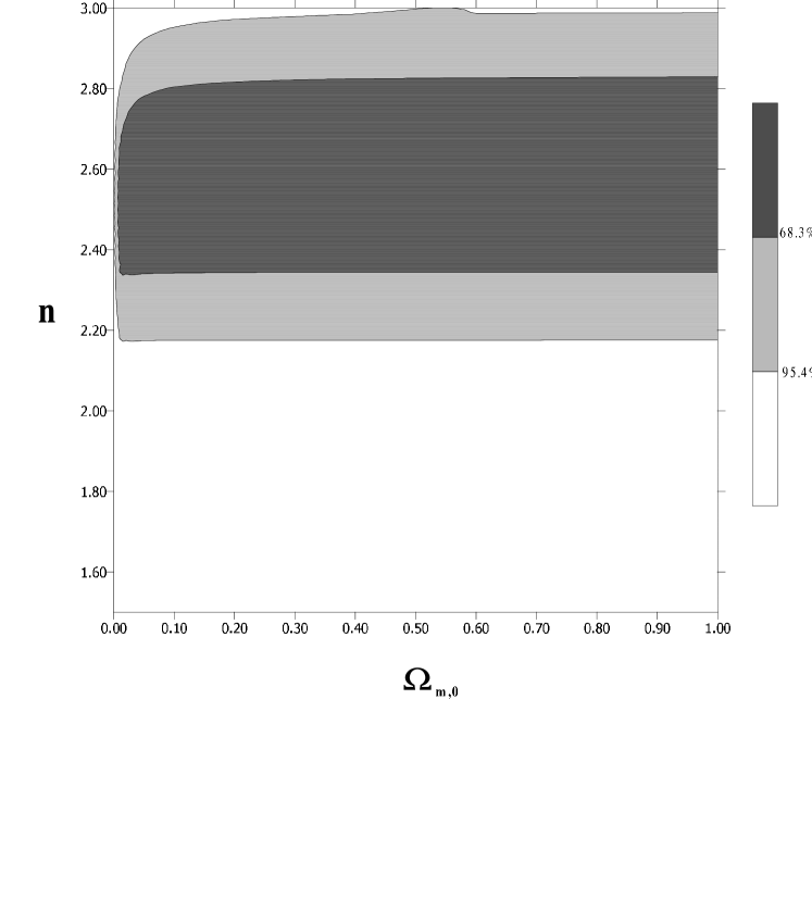
Figure 5: The flat non-linear gravity model ($w=0,n<3$). Confidence levels on the $(\Omega_{m,0},n)$ plane, marginalised over ${\cal M}$, obtained from SNIa Astier sample.

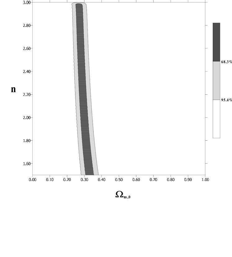
Figure 6: The flat non-linear gravity model ($w=0,n<3$). Confidence levels on the $(\Omega_{m,0},n)$ plane obtained from baryon oscillation peaks.

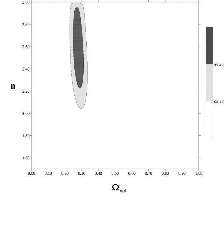
Figure 7: The flat non-linear gravity model ($w=0,n<3$). Common confidence levels on the plane $(\Omega_{m,0},n)$ obtained from SNIa Astier sample and baryon oscillations.

In modern observational cosmology, one encounters the so-called degeneracy problem: many models with dramatically different scenarios (big bang or bounce, big-rip or de Sitter phase) agree with the present day observational data. Information criteria for model selection Liddle:2004nh can be used, in some subclass of dark energy models, in order to overcome this degeneracy Godlowski05 ; Szydlowski06 . Among these, Akaike (AIC) Akaike:1974 and Bayesian (BIC) information criteria Schwarz:1978 are the most popular. From these criteria one can determine several essential model parameters, providing the preferred fit to the data Liddle:2004nh .

The AIC Akaike:1974 is defined by

$$\mathrm{AIC}=-2\ln{\mathcal{L}}+2d\ ,$$ (25)

where $\mathcal{L}$ is the maximum likelihood and $d$ the number of model parameters. The best model, with a parameter set providing the preferred fit to the data, is that which minimizes the AIC.

The BIC introduced by Schwarz Schwarz:1978 is defined as

$$\mathrm{BIC}=-2\ln{\mathcal{L}}+d\ln{N}\ ,$$ (26)

where $N$ is the number of data points used in the fit. While AIC tends to favor models with a large number of parameters, the BIC penalizes them more strongly, so the later provides a useful approximation to the full evidence in the case of no prior on the set of model parameters Parkinson:2005 .

The effectiveness of using these criteria in the current cosmological applications has been recently demonstrated by Liddle Liddle:2004nh . Analyzing CMBR WMAP satellite data Bennett:2003bz , he found the number of essential cosmological parameters to be five. Moreover, he came to important conclusion that spatially-flat models are statistically preferred to close models as it was indicated by the CMBR WMAP analysis (their best-fit value is $\Omega_{tot,0}\equiv\Sigma_{i}\Omega_{i,0}=1.02\pm 0.02$ at $1\sigma$ level).

In the paper by Parkinson et al. Parkinson:2005 , also the usefulness of Bayesian model selection criteria in the context of testing for double inflation with WMAP was demonstrated. These criteria were also used recently by us to show that models with the big-bang scenario are rather preferred over the bouncing scenario Szydlowski:2005qb .

Please note that both information criteria make no absolute sense and only the relative values between different models are physically interesting. For the BIC a difference of $2$ is treated as a positive evidence ($6$ as a strong evidence) against the model with larger value of BIC Jeffreys:1961 ; Mukherjee:1998wp . Therefore one can order all models, which belong to the ensemble of dark energy models, following the AIC and BIC values. If we do not find any positive evidence from information criteria, the models are treated as identical, while eventually additional parameters are treated as not significant. Therefore, the information criteria offer a possibility to introduce a relation of weak ordering among considered models.

Table 4: Results of AIC and BIC performed on the Astier versus the Gold Riess samples of SNIa.

sample	AIC	BIC
$\Lambda$CDM Gold	179.9	186.0
$\Lambda$CDM Astier	111.8	117.3
Non-Lin.Grav. Gold	186.6	195.8
Non-Lin.Grav. Astier	114.7	122.9

For comparizing the $\Lambda$CDM and the non-linear gravity models the results of AIC and BIC are presented in Tables 4. Note that for both samples we obtain with AIC and BIC for the $\Lambda$CDM model smaller values than for non-linear gravity. We use a Bayesian framework to compare the cosmological models, because they automatically penalize models with more parameters to fit the data. Based on these simple information criteria, we find that the SNIa data still favour the $\Lambda$CDM model, because under a similar quality of the fit for both models, the $\Lambda$CDM contains fewer parameters.

It is interesting that both models give different predictions for the brightness of the distant supernovae (see Fig. 3). The model of modified non-linear gravity predicts that very high redshift supernovae should be fainter than predicted by $\Lambda$CDM. So, we can expect future SNIa data to allow us discriminating finally between these two models.

IV Conclusion

The main subject of our paper has been to confront the simplest class of non-linear gravity models versus the observation of distant type Ia supernovae and the recent detection of the baryon acoustic peak in the Sloan Digital Sky Survey data. We find strong constraints on two independent model parameters ($\Omega_{m,0},\,n$). If we assume n=1, then we obtain the standard Einstein de Sitter model filled by both matter and radiation. We estimate model parameters using standard minimization procedure based on the likelihood function as well as the best fit method. For deeper statistical analysis, we have used AIC and BIC information criteria of model comparison and selection. Our general conclusion is that non-linear gravity fits well (both SNIa and baryon oscillation data). In particular we conclude:

1. Analysis of SNIa Astier data shows that values of $\chi^{2}$ statistic are comparable for both $\Lambda$CDM and best fitted non-linear gravity model.

2. The non-linear gravity models with $n<2$ can be excluded by combined analysis of both SNIa data and baryon oscillation peak detected in the SDSS Luminous Red Galaxy survey of Eisenstein at al. Eisenstein:2005 on $2\sigma$ confidence level.

3. From SNIa data we obtain a weak dependence of the quality of fits on the value of density parameter for matter ($\Omega_{m,0}$). However, the combined analysis allowed only value of $\Omega_{m,0}$ well tuned to its canonical value $\Omega_{m,0}=0.3$. This value of course is in good agreement with present extra-galactic data Peebles:2002gy .

4. We use the Akaike and Bayesian information criteria for comparison and discrimination between the analyzed models. We find these criteria still to favour the $\Lambda$CDM model over non-linear gravity, because (under the similar quality of the fit for both models) the $\Lambda$CDM model contains one parameter less.

5. The Hubble diagram implies that very high redshifted supernovae ($z\geq 1.5$) should be fainter in non-linear gravity model than those predicted by $\Lambda$CDM. So, future SNIa data can allow us finally to discriminate between these two models.

6. The standard general relativity models with $n=1$ (without cosmological constant) can be excluded by SNIa data on $17\sigma$ level (as the E-deS model).

7. The non-linear cosmology can therefore be treated as a serious alternative versus cosmology with dark energy of unknown nature.

V Acknowledgements

Authors thank Dr A.G. Riess and Dr P. Astier for the detailed explanation of their supernovae samples. We also thank Dr M. Fairbairn, Dr S. Capozziello and Dr K. Just for helpful discussion. M. Szydlowski acknowledges the support by KBN grant no. 1 P03D 003 26. A. Borowiec is supported by KBN grant no. 1 P03B 01 828.

References

- (1) A. G. Riess, Astron. J. 116 (1998) 1009.
- (2) S. Perlmutter, et al., Astrophys. J. 517 (1999) 565.
- (3) Weinberg S. Rev. Modern Phys. 61 (1989) 1.
- (4) S. M. Carroll, W. H. Press, E. L. Turner Ann. Rev. Astron. Astrophys. 30 (1992) 499.
- (5) R. G. Vishwakarma, P. Singh, Class. Quant. Grav. 18 (2001) 1159.
- (6) B. Ratra, P. J. E. Peebles, Phys. Rev. D37 (1998) 3406.
- (7) R. R. Caldwell, Phys. Lett. B545 (2002) 23.
- (8) M. P. Dabrowski, T. Stachowiak, M. Szydlowski, Phys.Rev.D68 (2003) 103519.
- (9) A. Y. Kamenshchik, U. Moschella, V. Pasquier, Phys. Lett. B511 (2001) 265.
- (10) K. Freese, M. Lewis, Phys. Lett. B540 (2002) 1.
- (11) S. Nojiri, S.D. Odintsov, hep-th/0601213. E.J. Copeland, M. Sami, S. Tsujikawa: hep-th/0603057; S. Bludman: astro-phys/0605198
- (12) S. Capozziello, Int. J. Mod. Phys. D11 (2002), 483.
- (13) S.M. Carroll, A. De Felice, V. Duvvuri, D.A. Easson, M. Trodden and M. Turner, Phys. Rev D71, (2005) 063513
- (14) G. Allemandi, A. Borowiec, M. Francaviglia, Phys. Rev D70, (2004) 043524
- (15) G. Allemandi, A. Borowiec, M. Francaviglia, Phys. Rev D70, (2004) 103503; G. Allemandi, A. Borowiec, M. Francaviglia, S. Odintsov, Phys. Rev D72, (2005) 063505
- (16) S. Capozziello, V.F. Cardone, M.Francaviglia, Gen. Relativ. Gravit. (2006) 38(5), 711.
- (17) M.Amarzguioui, O. Elgaroy, D.F. Mota and T. Multamaki: astro-ph/0510519; T. Koivisto, D.F. Mota, Phys.Rev. D73 (2006) 083502; T. Koivisto, Phys.Rev. D73 (2006) 083517; T. Sotiriou, Class.Quant.Grav.23 (2006) 1253-1267
- (18) A. G. Riess, et al., Astrophys. J. 607 (2004) 665.
- (19) P. Astier, et al., (2005) astro-ph/0510447
- (20) D. Eisenstein et al. (2005) astro-ph/0501171
- (21) O. Mena, J. Santiago, J. Weller, Phys.Rev.Lett.96 (2006) 041103; T. Biswas, A. Mazumdar, W. Siegel, JCAP 0603:009 (2006); R. Maartens, E. Majerotto: astro-phys/0603353; J. Ellis, N.E. Mavromatos, V.A. Mitsou, D.V. Nanopoulos: astro-ph/0604272; M.C. Bento, O. Bertolami , M.J. Reboucas, N.M.C. Santos: astro-ph/0603848; S. Capozziello, V.F. Cardone, A.Troisi: astro-ph/0603522; S. Capozziello, A. Stabile, A. Troisi: gr-qc/0603071; S. Capozziello, V.F. Cardone, A. Troisi: astro-ph/0602349
- (22) T. Clifton, J.D. Barrow, Phys. Rev D72, (2005) 103005
- (23) S. Carloni, P.K.S. Dunsby, S. Capozziello, Class. Quant. Grav 22 (2005) 4839
- (24) M. Fairbairn and A. Goobar (2005) astro-ph/0511029
- (25) A. R. Liddle, Mon. Not. Roy. Astron. Soc. 351 (2004) L49.
- (26) W. Godlowski, M. Szydlowski, Phys. Lett. B623 (2005) 10.
- (27) M. Szydlowski, W. Godlowski, Phys. Lett. B633 (2006) 427.
- (28) H. Akaike, IEEE Trans. Auto. Control 19 (1974) 716.
- (29) G. Schwarz, Annals of Statistics 6 (1978) 461.
- (30) D. Parkinson, S. Tsujikawa, B. Basset, L. Amendola, Phys Rev D71 (2005) 063524.
- (31) C. L. Bennett, et al., Astrophys. J. Suppl. 148 (2003) 1.
- (32) M. Szydlowski, W. Godlowski, A. Krawiec, J. Golbiak, Phys. Rev. D72 (2005) 063504.
- (33) H. Jeffreys, Theory of Probability, 3rd Edition, Oxford University Press, Oxford, 1961.
- (34) S. Mukherjee, E. D. Feigelson, G. J. Babu, F. Murtagh, C. Fraley, A. Raftery, Astrophys. J. 508 (1998) 314.
- (35) P. J. E. Peebles, B. Ratra, Rev. Mod. Phys. 75 (2003) 559.