Fourier resolved spectroscopy of 4U 1543–47 during the 2002 outburst

Abstract

We have obtained Fourier-resolved spectra of the black-hole binary 4U 1543–47 in the canonical states (high/soft, very high, intermediate and low/hard) observed in this source during the decay of an outburst that took place in 2002. Our objective is to investigate the variability of the spectral components generally used to describe the energy spectra of black-hole systems, namely a disk component, a power-law component attributed to Comptonization by a hot corona and the contribution of the iron line due to reprocessing of the high energy ($E\mathbin{\lower 3.0pt\hbox{$\hbox to0.0pt{\raise 5.0pt\hbox{$\char 62\relax$}\hss}\mathchar 29208\relax$}}7$ keV) radiation. We find that i) the disk component is not variable on time scales shorter than $\sim$ 100 seconds, ii) the reprocessing emission as manifest by the variability of the Fe K$\alpha$ line responds to the primary radiation variations down to time scales of $\sim 70$ ms in the high and very-high states, but longer than 2 s in the low state, iii) the low-frequency QPOs are associated with variations of the X-ray power law spectral component and not to the disk component and iv) the spectra corresponding to the highest Fourier frequency are the hardest (show the flatter spectra) at a given spectral state. These results question models that explain the observed power spectra as due to modulations of the accretion rate alone, as such models do not provide any apparent reason for a Fourier frequency dependence of the power law spectral indices.

1 Introduction

4U 1543–47 belongs to the group of black-hole X-ray novae (Tanaka & Shibazaki, 1996; Cherepashchuk, 2000). These are transient X-ray binaries in which the compact companion is a black hole and the optical companion a late-type star. They owe their name to the fact that they occasionally exhibit a large increase of their X-ray luminosity (i.e. outbursts), presumably due to a sudden increase of the mass accretion rate onto the black hole. At the peak of the outburst the X-ray luminosity may reach the Eddington limit. In 4U 1543–47 these outbursts are recurrent with a quasiperiod of 10-12 years. Previous outbursts have been observed in 1971 (Matilsky et al., 1972), 1983 (Kitamoto et al., 1984; van der Woerd et al., 1989), 1992 (Harmon et al., 1992) and 2002 (Park et al., 2004; Kalemci et al., 2005).

The first report on the observation of the optical counterpart to 4U 1543–47 was given by Pedersen (1983). Orosz et al. (1998) measured the radial velocity curve of the system and derived a mass function $f(M)=0.22\pm 0.02$, an orbital period of $P_{\rm orb}=1.123\pm 0.008$ days and estimated the distance to be 9.1$\pm$0.1 kpc. They argued that if the secondary star has a mass near the main sequence values for early A stars (Chevalier & Ilovaisky, 1992) then the mass of the primary must be in the range 2.7-7.5 ${\rm M}_{\odot}$. Recently, Park et al. (2004) gave a value of $9.4\pm 2{\rm M}_{\odot}$ (based on work in preparation by J. Orosz). Thus 4U 1543–47 is very likely to contain a black hole.

Additional evidence of the presence of a black hole in 4U 1543–47  is provided by the specific sequence of X-ray spectral states that the system follows as its outbursts evolve, usually associated with accretion onto black holes. At the peak of its recent outburst, while the $2-10$ keV flux was a large fraction of the Eddington luminosity, the source exhibited a soft, thermally dominated spectrum and little variability, i.e. it was in the High/Soft or thermally dominated state (HS; van der Klis (2005); McClintock & Remillard (2004)). As the flux decreased, the source entered the Very High or steep power-law dominated state (VHS), characterized by broad-band variability, increased contribution of the power-law flux and the presence of QPOs. At the end of the VHS the source showed a sharp increase in the power-law flux and rms amplitude of variability without a noticeable change in the photon index. According to Kalemci et al. (2005), 4U 1543–47 entered the intermediate state (IS). Just before the quiescent state the source went through the Low/Hard state (LS). At this state the thermal component was almost absent, the spectrum was dominated by the power-law, and the power spectrum displayed a simple broken power-law shape with rms of $\sim$20-30%.

The X-ray spectral and timing evolution of the source during its 2002 outburst has been studied in detail by Park et al. (2004) (HS, VHS and IS), Kalemci et al. (2005) (IS and LS) and La Palombara & Mereghetti (2005) (quiescent state). The outburst started around June 15, 2002, and lasted for over one and a half months. Park et al. (2004) used 49 RXTE observations that were obtained during the first 35 days of the outburst, while Kalemci et al. (2005) used 39 observations that were taken $\sim 25$ days after the onset of the outburst.

In the present work we use archival RXTE data collected at various epochs during the latest outburst of 4U 1543–47. Our aim is to study its Fourier resolved spectra at various frequency bands during the different spectral states which the source attains during the evolution of the outburst. This latter fact provides the opportunity of studying the variability properties of the different spectral components of accreting compact objects (i.e. power law, disk emission and iron line) in different spectral states of the same object, thus eliminating the ambiguities of referring to specific states at different objects with different masses and different Eddington ratios at specific luminosities.

Our study explores the variability properties on short time scales ($\sim 100$ sec) compared to those of recent studies (Park et al., 2004; Kalemci et al., 2005) that investigated the variability properties of the above spectral components on time scales of $\sim 1$ day (the typical time interval between successive RXTE observations). Our work follows the lines of a similar study by Revnivtsev et al. (1999) and Gilfanov et al. (2000) who explored the spectral variability of Cyg X-1 over similar time scales ($\sim 0.01-100$ sec) during the different spectral states of the source. A similar approach was also used by Papadakis et al. (2005), who studied the spectra of the AGN MCG 6-30-15.

While we examine the variability properties of the entire spectrum, we pay particular emphasis on those of the Fe K$\alpha$ line; the variation of this feature, due almost exclusively to the reprocessing of the harder X-ray radiation, is most sensitive to the geometry of reprocessing matter in the vicinity of the accreting object and it can be used to infer its structure.

In §2 we outline the details of our observations and data reduction procedure, while in §3 we present the results of our analysis. In §4 we discuss in detail the results of the variability of each spectral component and we comment on its significance and implications on the dynamics and geometry of the accreting matter while in §5 we outline our general conclusions.

2 Observations and Data Reduction

We obtained a total of approximately 60 ksec of data from the RXTE archives spanning June 18 to August 4, 2002, thus sampling the outburst from near its peak to well into the late decline stages. Typical count rates (PCA instrument) ranged $\sim 10^{4}$ near outburst peak to $\sim 10^{2}$ at the late decline phase. All the data were obtained from RXTE program IDs P70133 and P70124, the latter covering the decline phase of the outburst.

Data recording and packing in RXTE can be done in many different ways depending on the brightness of the source and the spectral and timing resolution requested. The specific observational modes are selected by the observer and may change during the overall observation. In order to ensure homogeneity in the reduction process the energy resolution was restricted to be 16 channels covering the energy band 2-15 keV, as this configuration could be achieved during the entire duration of the outburst.

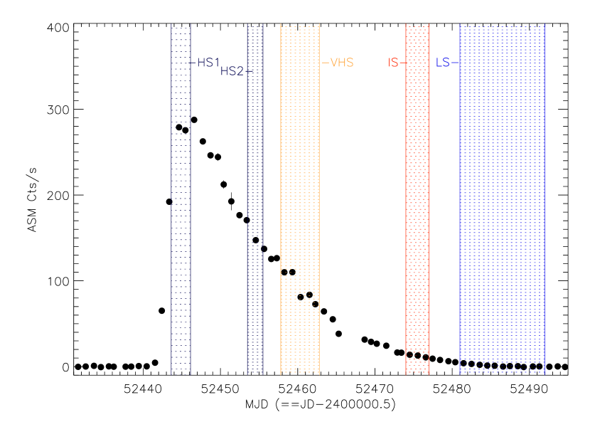
Figure 1: Plot of the $2-12$ keV ASM light curve. The shaded boxes indicate the time periods that we selected in order to extract data from the pointed RXTE observations within these periods.

Fig. 1 shows a plot of the daily average, $2-12$ keV, ASM light curve of the source during its outburst. For the purposes of the present work we have selected five observing intervals corresponding to four different spectral states of the source, according to the classification of Park et al. (2004) and Kalemci et al. (2005). These are shown with the shaded boxes in Fig. 1.

The first interval includes the two time ranges MJD 52443.7-52446.1 and MJD 52453.5-52455.1 (which we refer to as HS1 and HS2, respectively), during which the source was in its HS. The total on-source times were $\sim 18.4$ ksec and $\sim 7.6$ ks respectively. Note that the HS2 period is rather close to the chosen VHS time interval, while the HS1 period covers part of the rise. In this way we can investigate possible differences in the variability behavior of the source while in its high state. The second interval spans MJD 52457.8-52460.5 and corresponds to a period when the source was at its VHS. It contained 6 observations, amounting to 10.9 ks. We also considered four observations between MJD 52474.2 and 52477.2, which correspond to the IS between the VHS and the LS. Note, however, that the three observing intervals on July 21 2002 (MJD 52476; program ID P70132) were not included in our analysis because a different onboard spectral (and time) binning was used. Finally, ten observations between MJD 52481.1 and 52491.5 which corresponds to the LS of the source. The observing time for the IS and LS were 6.9 and 13.3 ksec, respectively.

Light curves were extracted for each onboard channel range using the current RXTE software, binned at a resolution of 0.015625 s. We then divided the data into 128-s segments and, following the prescription of Revnivtsev et al. (1999), we obtained the Fourier resolved spectra of the source in the following broad frequency bands: 0.008-0.5 Hz, 0.5-5 Hz and 5-15 Hz.

Contrary to typical temporal studies which provide the Power Spectral Densities (PSD) of the source in an entire energy band, Fourier resolved spectra provides instead the source spectra at different Fourier frequency ranges. This method consists of producing the PSD for every energy bin of the spectrum (i.e. the energy-dependent rms amplitude) and then weighing each bin in the energy spectrum with the corresponding rms amplitude.

2.1 Energy spectral analysis

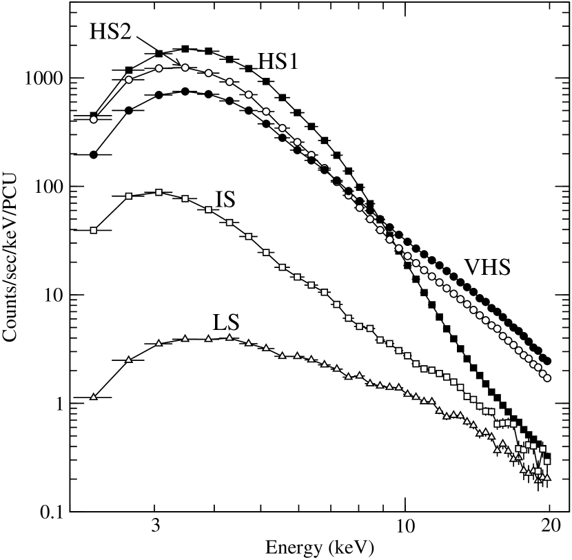
Figure 2: Plot of the $2-20$ keV energy spectra of the source during the various spectral states. The spectra have been labeled accordingly, and are divided by the number of the PCU units that were operated in each period.

Fig. 2 shows typical $2-20$ keV energy spectra of the source corresponding to the observational periods selected. The spectra were extracted from PCA Standard 2 mode data. The response matrix and background models were created using the standard HEADAS software, version 5.3. The number of detectors (PCU) that were switched on varied for each observation, and, in order to be able to compare the spectra, they were divided by the respective number of PCUs.

The filled squares and open circles in Fig. 2 show the spectrum of the source in the HS (HS1 and HS2, respectively), using data from the observations June 19 (when the source reached its maximum flux) and June 28, 2002 (Obs. No. 5 and 16 in Park et al., 2004). Open circles and open squares in the same figure show representative spectra of the source during the VHS and IS, respectively, using data from the observations performed in July 4 and 19, 2002 (Obs. No. 22 and 44 in Park et al., 2004). Finally, the open triangles show a representative LS spectrum, using data taken in August 1, 2002 (Obs. No. 19B in Kalemci et al., 2005). The spectral evolution with time is apparent in this figure. The HS spectra are characterized by a dominant thermal black body and a weak, steep power law component. The power-law flux increases during the VHS, and becomes the dominant component in the LS. As the total flux of the source decreases, the power-law slope becomes harder.

Although the spectral evolution of the source has been studied extensively in the past, we fitted the spectra using the same model components as in Park et al. (2004); Kalemci et al. (2005), i.e. a wabs model, to take account of the interstellar absorption effects (with $N_{H}=4.1\times 10^{21}$ cm^-2 that was kept fixed, Park et al. (2004)), a multicolor blackbody accretion disk model (Mitsuda et al., 1984; Makishima et al., 1986), a power-law model, a narrow Gaussian line (i.e. $\sigma$ fixed at 0.1 keV, smaller than the spectral resolution of RXTE) to account for the iron K$\alpha$ line emission, and a broad smeared absorption edge model (smedge in XSPEC, with the width fixed at 7 keV, like in Park et al. (2004)). The main reason to analyze the energy spectra is to reduce the spectral resolution of the Standard 2 spectra to match that of our Fourier-resolved spectra (i.e. 16 bins, in the 2-15 keV band, compared to $\sim$ 50 of the Standard 2 mode). This is a necessary step in order to be able to compare the results from the model fitting of the energy spectra with those from the model fitting of the Fourier-resolved spectra (presented in the following section).

The spectral analysis was performed using XSPEC version 11.3.1. We have added systematic errors of 1% to all channels and have restricted our analysis to the 2-15 keV band only (to match the energy band used in the case of the Fourier-resolve spectra). Our results are listed in Table 1. The errors quoted for the best fit values correspond to the 90% confidence limit for one interesting parameter. In the case when the error is large enough and the best-fit parameter value is consistent with being zero, we simply note the best-fit value plus upper error, and we accept it as the upper 90% limit for the respective parameter.

Our results are entirely consistent with those reported by Park et al. (2004); Kalemci et al. (2005) for the respective observations. In the case of the HS, VHS and IS spectra, our best-fit estimate of the equivalent width (EW) of the iron emission line is systematically smaller than that reported by Park et al. (2004), the main reason being the use of a narrow Gaussian line model in our case (which fits well the reduced resolution spectra that we are using).

Note that in the case of the LS spectrum, the addition of a narrow Gaussian line at $\sim 6.4$ keV to the single power-law fit reduces the $\chi^{2}$ by 9.7 (for two additional parameters), which is significant at the 91% level.

3 Fourier resolved spectral analysis

The usefulness of the frequency-resolved spectra lies on the fact that they receive significant contribution only from the spectral components that are variable on the time scales sampled by the observations. Therefore by performing Fourier-resolved spectroscopy we can investigate whether the various spectral components in the overall spectrum of the source (i.e. disk black-body, power-law, iron line) are variable at each frequency range considered. In general, the interpretation of the Fourier resolved spectra is not unique and requires additional assumption about the cause of variability. However, for the case of the iron Fe K$\alpha$ line and the Compton reflection components which are thought to result from the reprocessing of higher energy ($E\geq 7$ keV) radiation and are filtered by the well understood light travel-time effects, the Fourier-resolved analysis can provide meaningful constraints on the geometry of reprocessing matter with respect to the source of the hard radiation.

In this section we present the results of our Fourier spectral fitting analysis for each spectral state and compare the resulting best-fit parameters to those of the previous section (i.e, those obtained from the average energy spectra). As before, XSPEC version 11.3.1 was used for the model fitting. Most spectral fits yielded residuals attributable to absorption from the Xenon L edge at 4.78 keV. In order to account for this instrumental feature, we included in all model fits a Gaussian line model with central peak at 4.5–5 keV and fixed width ($\sigma=0.1$). We have also added, in all cases, an absorption component ($N_{H}=4.1\times 10^{21}$ cm^-2). A uniform systematic error of 1% was added quadratically to the statistical error of all Fourier spectra in each energy channel. Errors quoted for the best-fit values correspond to the 90% confidence limit for one interesting parameter (or to 90% upper limits in the case when the errors are too large). We describe the results of our analysis for each of the source’s spectral states below.

3.1 The High/Soft State

We first fitted the HS1 and HS2 Fourier spectra with a simple power-law model. We found that this model did not provide an acceptable fit to any of the Fourier spectra (note that, due to the low variability amplitude during the high state, we could not estimate a high frequency Fourier spectrum for the HS1 data). In both cases, the residuals reveal the presence of an emission and absorption feature at $\sim 6-7$ and $\sim 7-9$ keV, respectively. We then fitted the Fourier spectra with a model that consists of a power law, a Gaussian line and an edge (a simple edge model provided a better fit than the smedge that was used in the case of the energy spectrum). The energy and depth of the edge and the line energy were allowed to float as free parameters, but were forced to be identical in all three Fourier spectra. The line normalization was allowed to float in the three spectra.

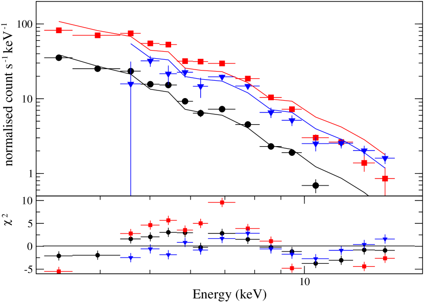
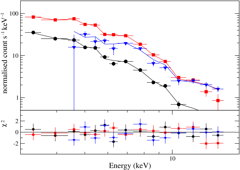
Figure 3: Energy spectra of the high state (HS) fitted to an absorbed power-law (left) and an absorbed power-law plus an iron line and edge (right). Different symbols represent different frequency ranges: 0.008-0.5 Hz (circles), 0.5-5 Hz (squares) and 5-15 Hz (triangles).

The best-fit parameter values for this model in the case of the HS1/HS2 spectra are listed in Table 2. Since they are consistent within the errors, we combined the individual HS1 and HS2 Fourier spectra and estimated the overall HS Fourier spectra. A simple power law model does not fit the data well ($\chi^{2}$ of 517 for 37 dof). The left panel in Fig. 3 shows the overall HS Fourier spectra, with the best-fit power-law model and the model residuals. The residuals clearly indicate the presence of a line emission and absorption edge features in the spectra. When these components are added to the model (see Fig. 3, right panel) the fit improves considerably ($\chi^{2}=31$ for 24 dof). The best-fit parameter values for this model are also listed in Table 2.

When the presence of the iron line is significant the equivalent width measured in the frequency-resolved spectra is larger than that found in the corresponding HS energy spectrum (listed in Table 1). Similarly, the best-fit edge energy of $\sim 9$ keV (a value representative of material with a high degree of ionization) appears to be significantly higher than the estimate of $7.5-8$ keV, reported in Table 1.

As for the best-fit power-law slopes, we observe a significant hardening with increasing frequency. Compared to the overall spectral slope of $\sim 2.5$ that characterizes the power-law component in the high state (Park et al., 2004), the low- and medium-frequency spectra are significantly steeper, while the high-frequency Fourier-spectrum slope is consistent with it.

3.2 The Very High State

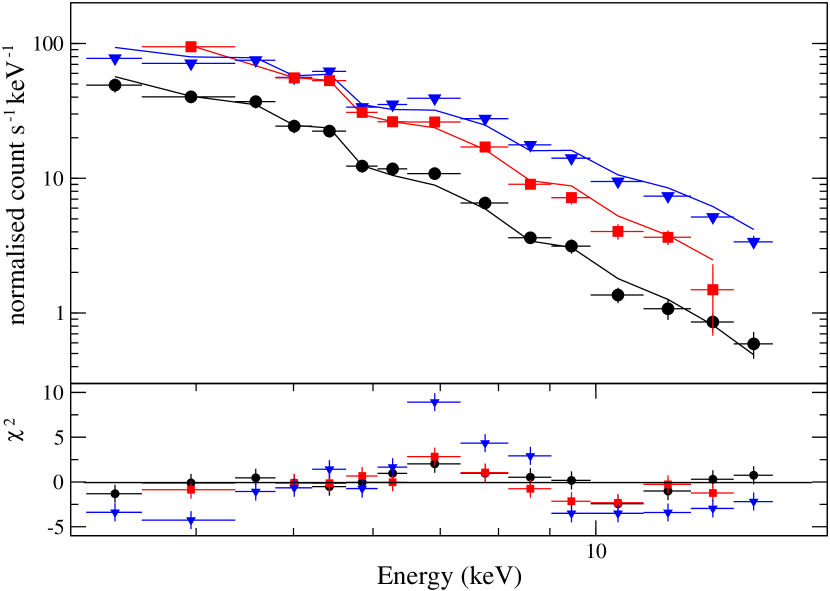
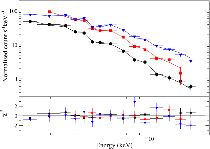
Figure 4: Energy spectra of the very high state (VHS) fitted to an absorbed power-law (left) and an absorbed power-law plus an iron line and edge (right). Symbols as in Fig. 3.

The left panel of Fig. 4 shows the best-fit power-law model to the VHS Fourier spectra. As with the HS spectra, it does not fit the data well ($\chi^{2}=210$ for 33 dof). Significant emission and absorption features appear at energies above $\sim 5-6$ keV. The right panel in Fig. 4 shows the three VHS frequency-resolved spectra with the best-fit ”power-law+Gaussian+absorption edge” model, which does provide a significantly better fit to the data ($\chi^{2}=29$ for 24 dof). The best-fit parameter values are listed in Table 2.

The iron line is clearly detected in the medium- and high-frequency spectra. Interestingly, the line energy is larger than the corresponding value in both the HS Fourier-spectra, and the VHS energy spectrum. The best-fit edge energy value is also larger than that in the VHS energy spectrum. In contrast, the edge optical depth in the VHS Fourier spectra appears to be smaller than in the VHS energy spectrum.

The power-law slope becomes harder as the frequency of the Fourier spectra increases. Compared to the overall power-law spectral slope, the low- and medium-frequency values are steeper by $\Delta\Gamma\sim 0.9-1$, while the high-frequency spectral slope is harder by $\Delta\Gamma\sim 0.2$.

3.3 The Intermediate and Low States

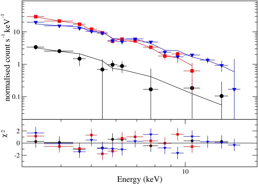
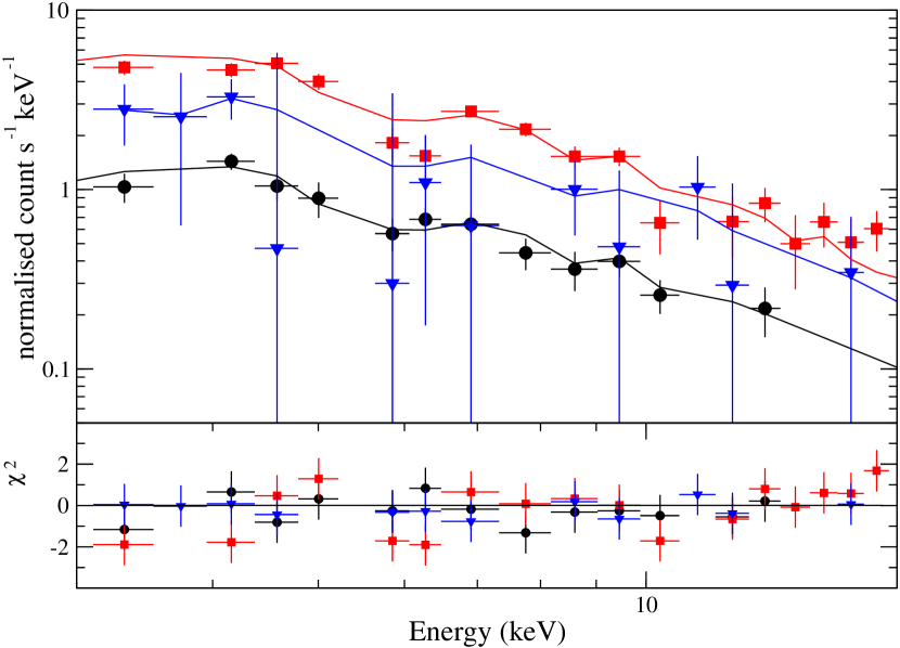
Figure 5: Energy spectra of the intermediate state (left) and hard/low state (right) fitted to an absorbed power-law model. Symbols as in Fig. 3.

The right and left panels in Fig. 5 show the best power-law model fits to the IS and LS Fourier spectra. In these cases, the model provides an acceptable fit ($\chi^{2}=30$ for 30 dof, and 32.6 for 24 dof, respectively). During the IS and LS observations the strength of the power law component increased, while its slope flattened reaching $\Gamma\sim 1.7$ during the LS period. Although the iron line and absorption edge are still present in the IS energy spectrum of the source, and the line may also be detectable in the energy spectrum during the LS (Table 1), these features are no longer evident in the Fourier resolved spectra, in marked contrast with the Fourier resolved spectra of the HS and VHS described above.

Looking at the residuals in the left panel of Fig. 5, one can see the same structure as in the HS and VHS, namely, the characteristic ”wiggle” in the 5-12 keV energy range (i.e., an excess of flux at about $6-8$ keV and a deficit at about 9 keV). For that reason we added a Gaussian line component in the IS model spectrum and we repeated the model fitting, keeping the line energy fixed to 6.4 keV. However, the quality of the fit did not improve significantly. We conclude that, if present, the strength of the iron line and the absorption edge must be significantly decreased, compared to that of the same features in the HS and VHS Fourier-spectra.

The spectral slope of the IS Fourier spectra is significantly steeper than the power-law slope in the respective Fourier spectra of the HS and VHS (by a factor of $\Delta\Gamma\sim 0.5-1$). The low- and medium-frequency IS Fourier spectra are steeper than the overall spectrum by $\Delta\Gamma\sim 1.5$. The high-frequency slope is flatter, but still steeper than the overall spectrum by $\Delta\Gamma\sim 0.6$. Finally, in the LS case, the flux of the source is too low to obtain a meaningful high-frequency (5–15 Hz) Fourier spectrum. The low- and medium-frequency spectra are slightly steeper than the overall energy spectrum ($\Delta\Gamma\sim 0.3-0.5$).

4 Discussion

In the previous sections we discussed our analysis and results of the Fourier Resolved Spectroscopy of 4U 1543-73 during the entire evolution of its 2002 outburst. The main goal of our work is to enlarge the sample of objects analyzed in this specific way, in an attempt to uncover and establish systematics associated with their spectro-temporal properties, different from the usual ones provided by simply their power spectral density (PSD). We found that a single power-law component does not provide good fits to most of the Fourier-resolved spectra and that the signatures typical of X-ray radiation reprocessing (such as iron line and edge) were required in order to obtain acceptable fits. In addition, no disk component was found in the Fourier-resolved spectra whose hardening with increasing frequency appears to be a general characteristic in all states. In this section we discuss the implications of these results and investigate the temporal properties of the model components that are generally used in black-hole spectral analysis.

4.1 The disk component

One of the most striking results of our analysis is the absence of variability in the multicolor blackbody disk component that provides the dominant flux in the observed HS and VHS spectra. The absence of variability in this component is manifest by the fact that the Fourier-resolved spectra are well fitted by a power law component only (plus an iron line and edge) when the system is in the HS and VHS. The fact that the contribution of the disk multicolor blackbody component is negligible in all Fourier-resolved spectra suggests that the disk is not variable on time scales shorter than $\sim$ 100 s. Even in the HS, when the disk is believed to extend down to the last stable orbit (and the variability time scales could indeed be short), the disk component is not required in the Fourier-resolved spectra at any of the frequency bands we examined.

This absence of variability is consistent with the magnitude of the viscous time scale of a disk with temperature $\simeq 1$ keV, estimated to be

$$\tau_{\rm vis} \simeq \frac{R_{S}}{c}x^{5/2}\frac{m_{p}c^{2}}{kT}\alpha^{-1}$$

$$\simeq 1.5\times 10^{3}\left(\frac{M}{10M_{\odot}}\right)\left(\frac{T}{1\;{\rm keV}}\right)^{-1}\alpha^{-1}\,{\rm sec}$$

where $x\simeq 3$ is the disk inner edge radius in units of the Schwarzschild radius ($R_{S}$) and $m_{p}$ is the proton mass. We conclude therefore that although the disk blackbody flux changes from day to day (see Fig. 2 in Park et al., 2004), the disk is stable on much shorter time scales (i.e. less than 100 sec). A similar result was also reported in the case of Cyg X–1 (Gilfanov et al., 2000), who found that the Fourier-resolved spectra of Cyg X–1 too are well fitted by a simple power-law component at all frequency bins, with no indication for a multi-color disk component, both when the system is in the High and Low States. The absence of rapid variability of the disk component, a result already noted by Miyamoto et al. (1994), appears to be a general trend in this class of objects.

This lack of disk variability puts constraints on models that attempt to attribute the observed PSDs as due to modulation of the accretion rate onto the compact object alone. At a minimum one would expect some variability of this component due to the reprocessing of the variable X-ray component on the disk and its re-emission as disk radiation. However, since the variable power law component represents only a small fraction of the disk luminosity, such variations, while presumably present, are hard to discern because of their small amplitude. For the same reason, we also believe that, at least in HS1, variations intrinsic to the disk, necessary for the dissipation of its kinetic energy, are too small to cause significant variations in its flux over the sampled time scales.

4.2 The iron line and edge

The results presented in §2.1 indicate the presence of a fluorescent K$\alpha$ iron line at $\sim$ 6.4 keV and an edge at $\sim 7-7.5$ keV in the HS, VHS and IS energy spectra, in agreement with the results of Park et al. (2004). These features constitute the main signatures for reflection in cold material of the primary source of X-rays. Our results presented in §3 exhibit the presence of similar features in the Fourier spectra for all frequencies (even the highest), when the source is in the HS and VHS (the fact that the line is not clearly detected in the low-frequency Fourier spectrum is almost certainly due to the fact that this spectrum has the lowest signal-to-noise among the three Fourier spectra). The Fourier-resolved spectra in the IS and LS are well fitted by a single power law model only. This implies that either the reflection features are absent or, if present, their strength must be significantly reduced when the system is in these states.

In the case of a conventional (i.e. non-Fourier resolved) energy spectrum, the equivalent width of the iron line (assuming that the reprocessing matter is neutral) is proportional to the ratio of the reflection component amplitude to that of primary radiation. However, the equivalent width of the iron line determined from a Fourier frequency resolved spectrum corresponds to the ratio of the rms variability amplitude of the reflected component to that of the primary emission variations in a given Fourier frequency range $\Delta\nu$, i.e., to the solid angle of the X-ray source subtended by reprocessing surface up to a length scale $L\mathbin{\lower 3.0pt\hbox{$\hbox to0.0pt{\raise 5.0pt\hbox{$\char 60\relax$}\hss}\mathchar 29208\relax$}}c/\Delta\nu$.

Our results show that the equivalent width of the line is $\sim 250-450$ eV at all frequency bins when the system is in the HS and VHS. This suggests that the reflected emission is fully responding to the primary radiation variations up to frequencies $\sim 15$ Hz, or to to time scales of $\simeq 70$ ms. On the other hand, our results also show that, when the system is in the IS and LS, the reflected component does not follow the primary emission variations on time scales shorter than 2 s (and perhaps even longer).

Gilfanov et al. (2000) reported similar results for Cyg X–1, when the source was in its HS and LS. They suggested that the most straightforward explanation of their results (and hence of ours as well) is in terms of a finite light-crossing time to the distance of the reflector. The equivalent width of the line in the Fourier-resolved spectra should remain roughly constant up to a frequency which corresponds to the inverse of the light travel time between the hard X-ray emitting corona and the inner radius of the disk that can reprocess the X-ray radiation into Fe K$\alpha$. Using Fig. 6 in Gilfanov et al. (2000), and the fact that the line equivalent width remains roughly constant up to frequencies $\sim 15$ Hz when the system is in the HS and VHS, we conclude that the innermost radius of the reflective material could be as low as $\sim 10R_{g}$ for a 10 M_⊙ black hole. The decrease of the line equivalent width in the IS and LS is consistent with the assumption that the accretion disk does not extend to small radii any longer.

In addition to the light travel time effect on the response of the iron line, the latter can be also influenced by the ionization sate of the reprocessing medium. As the latter increases, the energy of the iron line and associated edge increases (George & Fabian, 1991, and references therein). The larger values of the line energy in the VHS Fourier-spectra, $\sim 6.8$ keV, with respect to the VHS energy spectrum and the HS Fourier-spectra ($\sim 6.4$ keV in both cases) could then imply a higher degree of ionization in the innermost parts of the disk when the system is in the VHS. This is perhaps expected, since the power law component, which presumably illuminates the disk, has a larger luminosity during the VHS. Eventually, for sufficiently large values of the X-ray flux (more correctly of the ionization parameter) the reprocessing medium becomes highly ionized, resulting in suppression of both the Fe K$\alpha$ line and the Compton reflection features (Nayakshin et al., 2000).

4.3 The QPO

During the time interval MJD 52456–52461 Park et al. (2004) reported the detection of a QPO. The central frequency of the QPO varied in the range 7–10 Hz and the Q (coherence) parameter in 5-9 (i.e, a FWHM of $\mathbin{\lower 3.0pt\hbox{$\hbox to0.0pt{\raise 5.0pt\hbox{$\char 60\relax$}\hss}\mathchar 29208\relax$}}$ 2 Hz). However, when obtaining the average over the entire period when the QPO is present, the QPO extends over a wider frequency interval. In fact, we chose the high-frequency interval, namely 5–15 Hz, so as to cover all the frequency range of the QPO that appeared when the system was in the VHS. Therefore, the High-Frequency Fourier-resolved spectrum when the system is in the VHS should be representative of the energy spectrum of the variability components that “produce” the QPO in the system. The fact that no disk component is statistically required to fit this spectrum, implies that the QPO is not associated with the disk emission.

This result is in accordance with the behavior seen in most black hole systems (see e.g. Swank, 2001; McClintock & Remillard, 2004; van der Klis, 2005), namely that the QPO usually appears when the flux is dominated by the hard power-law component (there are no detected QPOs in the HS). The association between the QPO and the hard power-law is substantiated by the fact that the QPO amplitude increases with photon energy, when energy bands beyond the characteristic energy range of a multicolor blackbody with $kT\sim 1$ keV are considered (Belloni et al., 1997; Morgan et al., 1997). Muno et al. (1999) found that when the QPO is present, the power-law flux is much more variable than the disk flux. Only when the QPO is absent, the blackbody component is much more variable than the power law. In the case of 4U 1543–47, Kalemci et al. (2005) show that the QPO frequency does depend on the power law slope, and decreases with decreasing $\Gamma$, a correlation found to be generally present in accretion powered sources (Titarchuk & Fiorito, 2004).

4.4 The power-law component

A common effect seen in all three spectral states is the hardening of the power-law component with increasing frequency. That is, the X-ray emission associated with the variability of the shortest time scales is harder than that associated with the variability at longer time scales. Such a behavior is at first glance inconsistent with a model that attributes all variations to modulation of the accretion rate in a fashion that reproduces the observed PSDs. We do not see any obvious reason for such a behavior in the context of this type of model. This type of behavior is consistent with that observed by Revnivtsev et al. (1999) and Gilfanov et al. (2000) in Cygnus X-1 in its low-hard state. However, as pointed out in the latter work, the variable power law component of this source in its soft state is independent of the Fourier frequency, a fact not in complete agreement with the results of the present work.

A closer look at the results listed in Table 2 shows that at all states (except HS1) the high-frequency (HF) spectra are the hardest, while the power-law index of the low-frequency (LF) spectra is similar to that of the medium-frequency (MF) spectra, that is, $\Gamma_{\rm LF}\sim\Gamma_{\rm MF}$, while $\Gamma_{\rm{LF,MF}}>\Gamma_{\rm HF}$. In other words, we observe a rather large $\Delta\Gamma$ jump at frequencies higher than 5 Hz. This is the frequency at which the QPO appears. Furthermore, the 2-30 keV power spectrum during the HS and LS show a slope change at $\sim 5$ Hz - see upper left and bottom right plots in Fig.8 of Park et al. (2004). This feature is probably related to the dynamics of accretion, whose significance we are not able to assess at this point. However, it appears that the frequency range where the QPO lies presents a characteristic scale for this system that provides a demarcation of its spectral and timing properties.

Finally, we also observe that $\Gamma_{\rm LS}<\Gamma_{\rm{HS,VHS}}$ in the low and medium frequency bins. This correlation is generally observed among the different spectral states of accreting black holes, and is attributed to cooling of the corona temperature with the increased soft photon flux associated with the HS and VHS.

5 Conclusions

4U 1543–47 is the third (besides Cygnus X-1 and GX 339-4, Revnivtsev et al. (2001)) source amongst Galactic Black-Hole binaries for which Fourier resolved spectra have been calculated. The results from the energy spectral analysis of the three sources reveal several common characteristics, most importantly different spectral states characterized by soft and hard components, the former at higher luminosity than the latter.

Their Fourier resolved spectra at the corresponding spectral states exhibit also similarities: a) in the low/hard state the Fourier spectra tend to be harder with increasing Fourier frequency, while the Fe K$\alpha$ line is more prominent at lower Fourier frequencies. This result has been attributed to the size of the accretion disk inner radius, which may be set at distances $R\simeq 100R_{S}$ when the systems are in their LS. While this explanation can account for the absence of Fe line at high frequencies, it cannot account for the large value of the Fe line EW (in the case of Cyg X-1 for example) if the size of the X-ray emitting region is $\sim 10R_{S}$, as it is usually assumed. b) In the soft spectral states, the Fe line is present independent of the Fourier frequency. In the case of 4U 1543–47, we also observe a general hardening of the spectra with Fourier frequency in these states (different to Cyg X-1). c) A common characteristic of all Fourier resolved spectra (in all states) is the absence of the multicolor disk component in the Fourier resolved spectra, indicating that this component, while present, is not variable on time scales as short as a few hundred seconds. This results is in agreement with the viscous time scales of such disks.

In the case of 4U 1543–47, we also find evidence of an increased ionization state of the reflector when the system is in the VHS, while the absence of the disk component even in the QPO frequency range during the VHS, implies that the QPO emission is not associated with the disk emission.

The FRS technique provides a novel look at the structure of accretion powered sources. The general trends observed in the to-date analyses suggest common underlying systematics which are not fully yet understood. We believe that further analysis and modeling along the same lines for other sources is highly warranted.

Part of this work was supported by the General Secretariat of Research and Technology of Greece.

Table 1: Results from the model fits to the energy spectra ^a

Parameter	HS1	HS2	VHS	IS	LS
$T_{\rm col}$ (keV)	$0.99\pm 0.01$	$0.88\pm 0.02$	$0.87^{+0.02}_{-0.05}$	$0.6\pm 0.1$	$0.35^{b}$
$\Gamma$	$3.6\pm 0.2$	$2.6^{+0.2}_{-0.1}$	$2.7\pm 0.2$	$2.5\pm 0.1$	$1.73^{+0.04}_{-0.03}$
EFe (keV)	$6.2\pm 0.2$	$6.4\pm 0.2$	$6.3^{+0.2}_{-0.3}$	$6.5^{+0.1}_{-0.2}$	$6.3^{+0.2}_{-0.4}$
Eedge (keV)	$7.5\pm 0.1$	$7.8^{+0.7}_{-0.5}$	$7.5^{+0.6}_{-0.5}$	$7.1^{+0.3}_{-0.0}$	–
$\tau$	$1.4^{+0.1}_{-0.2}$	$0.8\pm 0.4$	$1.3^{+0.9}_{-0.2}$	$1.9^{+0.5}_{-1.2}$	–
EW(Fe) (eV)	$92\pm 8$	$91^{+8}_{-11}$	$90^{+22}_{-17}$	$210^{+195}_{-120}$	$<260$
$\chi^{2}_{\rm red}$/dof/prob	1.5/6/0.16	0.69/6/0.66	1.3/6/0.75	2.4/6/0.025	1.5/9/0.14

Table 2: Results from the model fits to the Fourier resolved spectra ^a

Parameter	HS1	HS2	HS	VHS	IS	LS
0.008–0.5 Hz
$\Gamma$	3.8${}^{+0.2}_{-0.2}$	3.2${}^{+0.3}_{-0.4}$	3.6${}^{+0.2}_{-0.2}$	3.6${}^{+0.1}_{-0.2}$	4.0${}^{+1.2}_{-0.9}$	2.2${}^{+0.3}_{-0.2}$
EFe (keV)	6.8${}^{+0.4}_{-0.6}$	6.4${}^{+0.4}_{-0.2}$	6.4${}^{+0.3}_{-0.2}$	6.8${}^{+0.1}_{-0.2}$	–	–
norm ($\times 10^{-4}$)	4${}^{+3}_{-3}$	$<4.7$	$<3.5$	$<7.3$	–	–
Eedge (keV)	9.2${}^{+0.3}_{-0.4}$	9.0${}^{+0.2}_{-0.2}$	9.0${}^{+0.2}_{-0.2}$	9.1${}^{+0.5}_{-0.3}$	–	–
$\tau$	0.8${}^{+0.5}_{-0.5}$	$<1.4$	1.1${}^{+0.5}_{-0.5}$	0.6${}^{+0.4}_{-0.2}$	–	–
EW(Fe) (eV)	$<1000$	$<1350$	$<575$	$<900$	–	–
0.5–5 Hz
$\Gamma$	3.1${}^{+0.3}_{-0.2}$	2.8${}^{+0.1}_{-0.1}$	3.0${}^{+0.1}_{-0.1}$	3.7${}^{+0.2}_{-0.2}$	4.2${}^{+0.1}_{-0.1}$	2.0${}^{+0.2}_{-0.1}$
EFe (keV)	6.8b	6.4b	6.4b	6.8b	–	–
norm ($\times 10^{-4}$)	9${}^{+7}_{-8}$	13${}^{+5}_{-5}$	19${}^{+6}_{-5}$	9${}^{+6}_{-6}$	–	–
Eedge (keV)	9.2b	9.0b	9.0b	9.1b	–	–
$\tau$	1.0${}^{+0.7}_{-0.6}$	1.1${}^{+0.2}_{-0.2}$	1.4${}^{+0.3}_{-0.3}$	$<0.56$	–	–
EW(Fe) (eV)	$<1000$	450${}^{+175}_{-175}$	435${}^{+205}_{-175}$	270${}^{+190}_{-165}$	–	–
5–15 Hz
$\Gamma$	–	2.4${}^{+0.2}_{-0.2}$	2.5${}^{+0.5}_{-0.7}$	2.5${}^{+0.1}_{-0.1}$	3.1${}^{+0.1}_{-0.1}$	–
EFe (keV)	–	6.4b	6.4b	6.8b	–	–
norm ($\times 10^{-4}$)	–	10${}^{+8}_{-7}$	$<25$	20${}^{+5}_{-5}$	–	–
Eedge (keV)	–	9.0b	9.0b	9.1b	–	–
$\tau$	–	1.0${}^{+0.4}_{-0.4}$	1.0${}^{+0.4}_{-0.4}$	0.3${}^{+0.1}_{-0.2}$	–	–
EW(Fe) (eV)	–	600${}^{+690}_{-390}$	–	390${}^{+160}_{-150}$	–	–
$\chi^{2}_{\rm red}$/dof/prob	0.54/17/0.93	1.30/24/0.15	1.22/25/0.21	1.21/24/0.22	1.01/30/0.45	1.36/24/0.11

References

- Belloni et al. (1997) Belloni, T., van der Klis, M., Lewin, W. H. G., et al. 1997, A&A, 322, 857
- Cherepashchuk (2000) Cherepashchuk A.M. 2000, SSRv, 93, 473
- Chevalier & Ilovaisky (1992) Chevalier, C. & Ilovaisky, S. A 1992, IAUC, 5520
- George & Fabian (1991) George, I.M. & Fabian, A.C. 1991, MNRAS, 249, 352
- Gilfanov et al. (2000) Gilfanov, M., Churazov, E. & Revnivtsev, M. 2000, MNRAS, 316, 923
- Harmon et al. (1992) Harmon, B. A., Wilson, R. B., Finger, M. H., Paciesas, W. S., Rubin, B. C., & Fishman, G. J. 1992, IAUC, 5504, 1
- Homan et al. (2001) Homan, J, Wijnands, R., van der Klis et al. 2001, ApJSS, 132, 377
- Kalemci et al. (2005) Kalemci, E., Tomsick, J. A., Buxton, M. M., Rothschild, R. E., Pottschmidt, K., Corbel, S., Brocksopp, C., & Kaaret, P. 2005, APJ, 622, 508
- Kitamoto et al. (1984) Kitamoto, S., Miyamoto, S., Tsunemi, H., Makishima, K., & Nakagawa, M. 1984, PASJ, 36, 799
- La Palombara & Mereghetti (2005) La Palombara, N. & Mereghetti, S. 2005, A&A, 430, L53
- Makishima et al. (1986) Makishima, K, Maejima, Y., Mitsuda, K., brandt, H.V., Remillard, R.A., Tuohy, I.R., Hoshi, R., & Nakagawa, M. 1986, ApJ, 308, 635
- Matilsky et al. (1972) Matilsky, T. A., Giacconi, R., Gursky, H., Kellogg, E. M., & Tananbaum, H. D. 1972, ApJ, 174, L53
- McClintock & Remillard (2004) McClintock, J.E. & Remillard, R. A, 2004, in Compact stellar X-ray sources, ed. W.H.G. Lewin, & M. van der Klis, Cambridge University Press.
- Mitsuda et al. (1984) Mitsuda, K.,Inoue, H., Koyama, K. et al. 1984, PASJ, 36, 741
- Miyamoto et al. (1994) Miyamoto, S., Kitamoto, S., Iga, S., Hayashida, K., & Terada, K. 1994, ApJ, 435, 398
- Morgan et al. (1997) Morgan, E.H., Remillard, R.A., & Greiner, J. 1997, ApJ,482, 993
- Muno et al. (1999) Muno, M.P., Morgan, E.H., & Remillard, R.A. 1999, ApJ, 527, 321
- Nayakshin et al. (2000) Nayakshin, S., Kazanas, D. & Kallman, T. R. 2000, ApJ, 537, 833
- Orosz et al. (1998) Orosz, J. A., Jain, R. K., Bailyn, C. D., McClintock, J. E., & Remillard, R. A. 1998, ApJ, 499, 375
- Park et al. (2004) Park, S.Q., Miller, J.M., McClintock, R.A., et al. 2004, ApJ, 610, 378
- Pedersen (1983) Pedersen, H. 1983, Messenger, 34, 21
- Papadakis et al. (2005) Papadakis, I. E., Kazanas, D., & Akylas, A. 2005, ApJ, 631, 727
- Revnivtsev et al. (1999) Revnivtsev, M., Gilfanov, M., & Churazov, E. 1999, A&A, 347, L23
- Revnivtsev et al. (2001) Revnivtsev, M., Gilfanov, M., & Churazov, E. 2001, A&A, 380, 502
- Swank (2001) Swank, J. 2001, ApSSS, 276, 201
- Tanaka & Shibazaki (1996) Tanaka, Y., & Shibazaki, N. 1996, ARA&A, 34, 607
- Titarchuk & Fiorito (2004) Titarchuk, L. G. & Fiorito, R. 2004, ApJ, 612, 988
- van der Klis (2005) van der Klis, M. 2005, in Compact Stellar X-ray sources, eds. W.H.G. Lewin, M. van der Klis,CUP, astro-ph/0410551
- van der Woerd et al. (1989) van der Woerd, H., White, N. E., & Kahn, S. M. 1989, ApJ, 344, 320