11email: marian.douspis@ias.u-psud.fr 22institutetext: Laboratoire d’Annecy-le-Vieux de Physique des Particules, UMR5814 CNRS, 9 Chemin de Bellevue, BP 110, F–74941 Annecy-le-Vieux cédex, France
22email: zolnierowski@lapp.in2p3.fr 33institutetext: LATT , Université de Toulouse, CNRS, 14 avenue É. Belin, F–31400 Toulouse, France
33email: alain.blanchard@ast.obs-mip.fr 44institutetext: CNRS, UMR 7095, Institut d’Astrophysique de Paris, Paris, F-75014 France ; Université Pierre et Marie Curie-Paris 6, UMR 7095, Paris, F-75014 France
44email: riazuelo@iap.fr
What can be learned about dark energy evolution?
We examine constraints obtained from SNIa surveys on a two parameter model of dark energy in which the equation of state undergoes a transition over a period significantly shorter than the Hubble time. We find that a transition between and (the first value being somewhat arbitrary) is allowed at redshifts as low as , despite the fact that data extend beyond . Surveys with the precision anticipated for space experiments should allow only slight improvement on this constraint, as a transition occurring at a redshift as low as could still remain undistinguishable from a standard cosmological constant. The addition of a prior on the matter density only modestly improves the constraints. Even deep space experiments would still fail to identify a rapid transition at a redshift above . These results illustrate that a Hubble diagram of distant SNIa alone will not reveal the actual nature of dark energy at a redshift above and that only the local dynamics of the quintessence field can be infered from a SNIa Hubble diagram. Combinations, however, seem to be very efficient: we found that the combination of present day CMB data and SNIa already excludes a transition at redshifts below .
Key Words.:
Cosmology – Cosmic microwave background – Supernovae – Cosmological parameters1 Introduction
The nature of dark energy is one of the most puzzling mysteries of modern cosmology. It is now widely accepted that our universe is experiencing a phase of accelerated expansion (Peebles & Ratra 2003). The evidence was first found using a type Ia supernovae luminosity vs. redshift diagram (Riess et al. 1998; Perlmutter et al. 1999), but a number of other observations now support this conclusion. In particular, estimations of the matter density of the universe generally lead to a low value, while the CMB anisotropies point toward a spatially flat Universe (Lineweaver et al. 1997; de Bernardis et al. 2000). WMAP data also require the presence of dark energy (Spergel et al. 2007) unless one considers an unexpectedly low value of the Hubble parameter (Blanchard et al. 2003; Hunt & Sarkar 2007). The possible correlation of the CMB fluctuation map with surveys of extragalactic objects (Fosalba et al. 2003; Corasaniti et al. 2005; Pogosian 2005) also provides direct evidence, although with a limited significance level (), for the existence of an unclustered dark energy component in the universe, the detected correlation being explainable through the integrated Sachs-Wolfe effect, i.e., a time variation of the gravitational potential, which is achieved only if the (baryonic + cold) matter density parameter significantly differs from 1. Finally, the shape of the correlation function on scales up to Mpc which has been recently measured accurately (Eisenstein et al. 2005) in combination with the CMB data advocates for the presence of dark energy (Blanchard et al. 2006) in the framework of general relativity. However, the nature of this dark energy has been the subject of numerous speculations. The simplest model, which was originally proposed (in another context) by Einstein (1917), is a pure cosmological constant , a term on the left hand side of Einstein’s equations. However, a cosmological constant can also be regarded as the contribution of the vacuum to the right hand side of the equation with a specific equation of state, i.e., a component with negative pressure related to the energy density by the relation . Indeed, quantum field theory predicts that the lowest energy state of any mode contributes to a vacuum energy density that behaves exactly as a cosmological constant (see, e.g. Binétruy 2000). A number of problems arise with this possibility, in particular the so-called hierarchy problem: the expected contribution is usually enormous, naive calculation gives , around 122 orders of magnitude larger than the present critical density of the universe. However, there exist mechanisms, such as supersymmetry, which allow one to reduce considerably the vacuum energy density, but since supersymmetry is broken at a scale larger than one is still plagued with an enormous vacuum energy density of the order of . The usual explanation is then to say that there exists a yet unknown mechanism which ensures that the contribution of the vacuum energy density is zero. One is therefore left to explain the nature of dark energy, which differs from a cosmological constant, avoiding the extreme fine tuning required to obtain the observed dark energy density (Binétruy 2000). Most models that have been proposed so far (quintessence models) therefore rely on the idea that some scalar field (Caldwell et al. 1998) behave today like a cosmological constant, exactly as an other scalar field did during inflation. The most remarkable feature of quintessence models is that both the scalar field pressure and energy density evolve according to dynamical equations. Consequently, the so-called equation of state parameter, , varies with time between and , as the field evolves along the potential. In some extreme (and possibly ill-defined) models, this parameter can even take any arbitrary value, for example if one allows the density to take negative values or a change in the sign of the kinetic term (Caldwell 2002). Other models involving scalar tensor theories also allow for such transient behaviour (Elizalde et al. 2004). The detection of such a variation would therefore be of great importance for our understanding of dark energy.
The aim of the present paper is to study models with a rapid transition of the equation of state and to illustrate that in this case, the Hubble diagram of SNIa provides surprisingly weak constraints compared to the case of a smooth transition. In Sec. 2, we recall a few basic aspects of simple quintessence models, and the motivation for a convenient parametrization of the equation of state parameter allowing rapid transition. In Sec. 3, we describe the analysis we perform, and state our main results. In Sec. 4 we discuss the crucial issue of the impact of the epoch of observation on the parameter estimation. We draw the main conclusions of our work in Sec. 5.
2 Dark energy parametrization
Historical quintessence models rely on the idea of a tracking solution (Ratra & Peebles 1988; Wetterich 1988), which involves a scalar field evolving in an inverse power law potential, , the proportionality constant being tuned so as to obtain the desired value of the dark energy density parameter today. The main feature of these models is that the pressure to energy density ratio, , remains constant both in the radiation era and in the matter era (with different values during each epoch), and that it tends toward once the quintessence energy density dominates. The value of the parameter depends on the power law index of its potential. From existing data, it seems that only values close to today, or even possibly lower, are acceptable (Caldwell 2002; Melchiorri et al. 2003). Note however that in the latter case, values of below cannot be obtained naturally through a standard scalar field. Single power law potentials suffer from the fact that, once quintessence dominates, the parameter approaches the asymptotic value very slowly so that today, if the quintessence density parameter is close to , then is still far from the value , contrary to what most analyses suggest. In order to avoid this problem, one has to add extra features in the potential, such as a rapid change in the slope of the potential or a local minimum, such as in the SUGRA model proposed by Brax & Martin (1999). Many other possibilities have been proposed since then (see for example references in Brax et al. 2000; Peebles & Ratra 2003).
On the other hand, without precise ideas about the correct quintessence model, it has become natural to adopt a more phenomenological approach in which one parametrizes the functional form of which exhibits the main features described above.
The simplest model of quintessence (in the sense that it introduces only one new parameter as compared to a CDM model) is to assume a constant . However there is little motivation for constant beyond the economical argument and it is increasingly recognized that evolving should be investigated with a minimal number of priors. In the absence of well motivated theoretical considerations one is left with the empirical option to examine constraints on the analytical form for . Most investigations have been based on expressions with one or two parameters. However, such expressions often vary with time in a relatively slow way and that rapidly varying expressions have to be examined as well. In other words, if one considers the typical time scale:
| (1) |
constant corresponds to where is the Hubble time, a smoothly varying expression such as the inverse power law potential corresponds to and a more rapidly varying correspond to , such as in the SUGRA model. Our aim is primarily to investigate constraints on models for which . This lead us to use the following model which allows arbitrary rapid transitions and in which the dark energy parameter evolves as a function of the scale factor according to
| (2) |
The parameter goes from at early times to at late times, the transition occurring at . The transition occurs at redshift (a negative value of which corresponds to a transition in the future) and lasts of the order of Hubble times; is therefore a parameter describing the speed of the transition : high values () correspond to fast transitions, in the limit the transition is instantaneous. This expression was proposed by Linder & Huterer (2005). The quintessence conservation equation can be integrated exactly to give
| (3) |
where we have set
| (4) |
and where corresponds to the values of the quintessence energy density at the present epoch. Therefore, the model can be implemented without much modification in existing cosmological codes such as CAMB (Lewis et al. 2000). Dark Energy perturbations are implemented accordingly to Riazuelo & Uzan (2002); Brax et al. (2000), i.e. the initial spectrum of the dark energy perturbation follows an attractor mechanism, exactly as the unperturbed part of the DE fluid does, and the DE initial spectrum is lost. One modification concerns the sound speed defined as which is equal to the parameter when is constant. When is not constant, as is the case for our model, its exact value is known since the analytic forms of and are known. This model has four parameters. As we said earlier, simple quintessence model have fewer: constant models correspond to , with undefined and . With an inverse power law potential, one has , , the epoch of transition is fixed approximately by the constraint and the duration of the transition is larger than the Hubble time (it depends on how steep the potential is, that is, on ). For the SUGRA potential the first two above constraints on and remain, whereas the latter are modified: the epoch of transition for no longer necessarily corresponds to the scalar field domination (but corresponds to the epoch where the field reaches a local minimum in its potential), and the transition duration is usually much shorter. Various other models have different predictions concerning these parameters, but the above parametrization is sufficiently general to encompass a large number of already proposed models.
One of these parameters, , is not expected to be as relevant as the parameter : because at early times is negligible compared to , the quintessence field does not play a crucial role, at least with respect to supernovae and CMB data. One should impose a value of slightly lower than 0, in order to ensure that at early times . The reason is that with and a low transition would be close to its present value at the recombination epoch (or even nucleosynthesis, see references in Peebles & Ratra 2003). At low redshift, this would lead to a dramatic suppression of the cosmological perturbation growth rate (Douspis et al. 2003). In addition, we found that this introduces additional changes in the curve at high (i.e., other than changes due to the modification of the angular distance). For these reasons we fix . Putting a constraint on is less desireable since it implicitly selects a limited class of models, which do not seem excluded by the data. We have chosen the value , which seems in agreement with the present data, and we focus on the two remaining parameters, and which describe the transition experienced by between its early and late behaviour.
3 Analysis
We focus here on constraints that can be set in the transition parameters and , and we set and as explained above. Note that a pure cosmological constant behaviour is obtained by considering large with a sufficiently small transition duration (so that it does not last long after ).
3.1 Supernovae Hubble diagram
The luminosity distance is one of the main sources of constraint on the nature of dark energy (Astier (2001)). We therefore first examine what kind of constraints the Supernovae Hubble diagram allows. The number of well observed SNIa has rapidly increased in recent years and a significant number of supernovae above redshift one have been detected. In the following we use the last compilation from Davis et al. (2007) of recent SNIa (Wood-Vasey et al. (2007); Riess et al. (2007); Astier et al. (2006)).
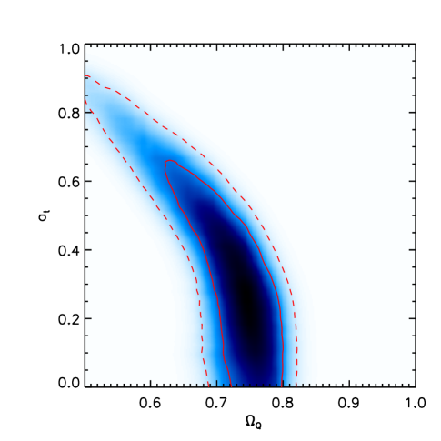
We have examined constraints on our three parameters, , and . We use the publicly available Monte Carlo Markov Chains code, cosmomc (Lewis & Bridle (2002)), using the modified version of CAMB described above. 2-D contours shown in Figures 1 and 4 encompass 68% and 95% confidence levels (CL). In each figure, the third parameter is marginalised over.
The upper graph of Figure 1 presents the allowed regions in the plane: versus the inverse duration of the transition . The lower graph gives the constraints in the – plane. Constraints on possible transitions appear very weak: only sharp transitions at very low redshift ( at the two sigma level) are firmly excluded. Surprisingly, the data suggest a transition at low redshift, a tendency that has been noticed elsewhere (Bassett et al. 2004; Corasaniti et al. 2004). However the significance level is low and a cosmological constant remains consistent with the data at the 2 sigma level.
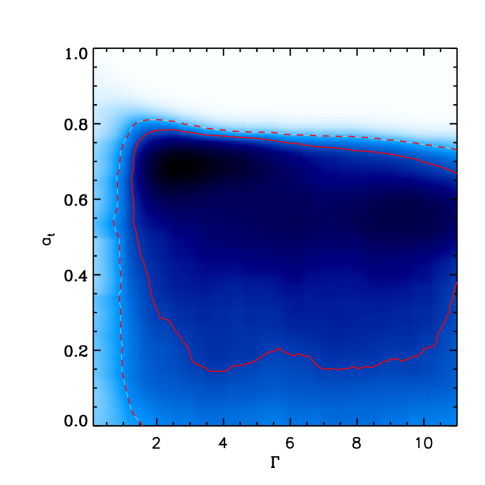
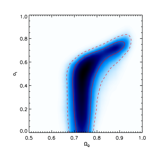
While rapid transitions (corresponding to large ) are very weakly constrained, better constraints are obtained when a strong prior is set on : with we found that transitions are acceptable at redshifts greater than . This improvement is due to the removing of degeneracy breaking (noticed in the parameter space of Figure 1) but remains modest. This means that the Hubble diagram of distant SNIa alone is insufficient to determine the nature of the dark energy at high redshift.
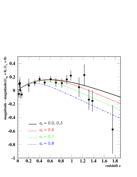
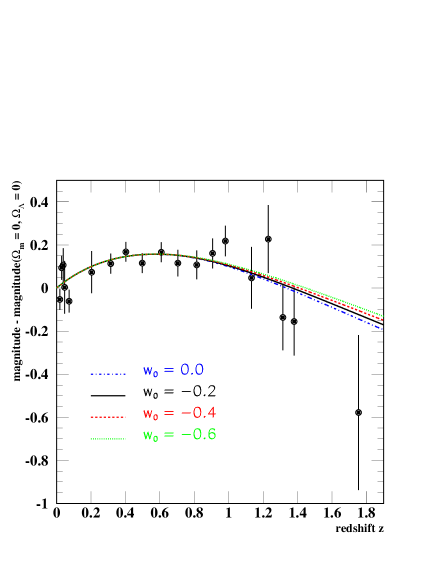
In Figures 2, we show the effect of a transition on the magnitude difference between a fiducial model and the empty universe, all other parameters being fixed with their fiducial values. The top figure clearly reveals that a transition from to occurring at even moderately low redshift makes very little differences to the observable quantity. It is therefore not surprising that the constraints that can be set from the present day SNIa Hubble diagram are not very tight. The bottom figure illustrates the effect of changing : changing from to produces changes that are small and easy to understand as the model becomes degenerate with the CDM model as tends to . For this reason, in the following, we concentrate our analysis on .
We have redone the above analysis on for a simulated survey with the precision and statistics expected from space experiments. We generated 2000 supernovae distributed in 16 bins in redshift between 0.2 and 1.7 according to Table 1 of Kim et al. (2004) completed by 300 nearby supernovae. The number of supernovae per bin fluctuates according to a Poisson law. For a given bin, the magnitude of the supernovae is taken from a Gaussian distribution of the mean value given by the standard concordance CDM model, and the sigma fixed to 0.2 magnitude. The resulting magnitude of each bin is obtained by a fit of the distribution of magnitudes and the associated error is added in quadrature with a systematic error of 0.02 magnitude and an offset error of 0.01 magnitude for the intercalibration between the two sets of data. The constraints inferred from this simulated sample again reveal that the transition epoch is moderately constrained: transitions at redshift as low as (2 CL) are still acceptable when a rapid transition () is assumed.
The situation is therefore paradoxical: although space survey precision improves the constraints by pushing the acceptable redshift from 0.25 to 0.5 (for rapid transitions), this last result is modest as a significant fraction of the high precision data provided by the experiment extends up to redshift . The reason for this apparent paradox is clarified in Sec. 4.
3.2 Constraints from the CMB
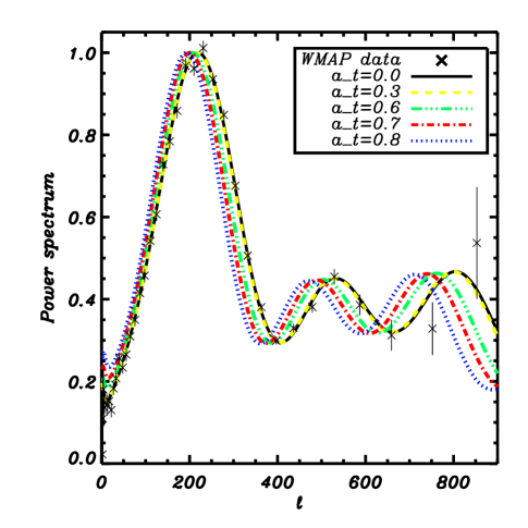
Given that SNIa Hubble diagram hardly suggests the presence of a transition in the dark energy content of the universe, it is interesting to examine whether such a possibility could be acceptable using additional constraints. CMB is known to provide such constraints on the quintessence scenario, eg (Spergel et al. 2003; Douspis et al. 2003; Ödman et al. 2004). We therefore examine CMB constraints on the type of models introduced above, although we leave to a future work a full investigation of the constraints that can be set on this type of model. We use the WMAP 3 data-set, as well as CBI, VSA and Boomerang data at small scales, and a version of the CAMB cosmological code (Lewis et al. 2000) that we have modified. Modifications of the code are straightforward since its public version includes models with constant in which we have implemented the energy density and the pressure as a function of redshift. Our ansatz for the equation of state parameter allows us to integrate the conservation equation to obtain an analytical form for 111One has also to make the distinction between the equation of state parameter and the “sound speed” squared , which are identical when is constant..
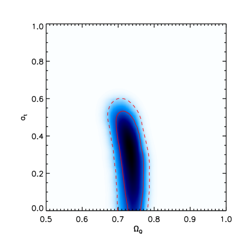
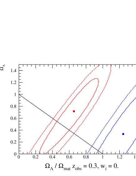
The angular power spectrum of CMB fluctuations in the presence of dark energy is modified mainly through the modification of the angular distance (Blanchard 1984) (see Fig. 3 and Elgarøy & Multamäki (2007)). Although a strong dependence appears, this is partially lost through parameter degeneracies which strongly weaken the final constraints. In addition, ISW will contribute to lower levels as the transition is assumed at lower redshift, and this effect contributes to modify the angular power spectrum of the CMB fluctuations. We have investigated the CMB constraints on models with rapid transitions described by Eq. 2. was set to 10. We have checked that varying above 5 produces no appreciable differences. The other parameters that were left free are the baryon budget , the optical depth , the Hubble constant , the dark energy density at the present day , the index of the primordial spectrum , the amplitude of fluctuations and the transition epoch . From the contours obtained in figure 4, one can see that the constraints that can be set on the transition redshift from the CMB are rather stringent, (1 on one parameter) when represents less than of the total density. These constraints being slightly dependent on we have also examined whether a combination of CMB and supernova data allows to improve the transition epoch constraints, but although the SNIa data restricted the dark energy density much more around , the final constraints do not represent a significant improvement: the final constraint shown in Figure 4 is (2 on one parameter). Some different dark energy models could in principle lead to different conclusions in the case where the sound speed varies in a way that significantly affects the integrated Sachs-Wolfe effect on large angular scales, even though no such model was found in our analysis. Clearly, better constraints could be obtained from additional data of cosmological relevance, but this is beyond the scope of the present paper.
4 Observing the Universe at and at
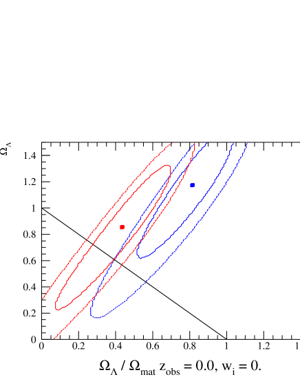
In order to distinguish quintessence models from a pure cosmological constant, it is crucial to be able to track the dark energy evolution as early as possible. The main impact of dark energy comes from its influence on the expansion rate of the universe. An important question is therefore until what epoch the dark energy density plays a role in observable quantities, and as a corollary, until what epoch one can hope to reconstruct either its energy density or its equation of state parameter. As we have seen in section 3, the SNIa Hubble diagram poorly constrains a possible transition epoch in the equation of state of the dark energy component. As we have stated, this appears somewhat paradoxical as data extending up to redshift 2 fail to reveal a transition occurring at redshifts as low as 0.25, at which the dark energy component is still dominant. Indeed, in a model with , today, with constant and equal to , the matter to dark energy transition, defined when , occurs at redshift . Let us now consider two alternatives. First, we can consider a pure cosmological constant model, with also at early times. Second, we can consider a model where for . In the first case, one has a usual CDM model, whereas in the second case, one has a model close to a flat Einstein-de Sitter model at epoch . An observer at should easily be able to distinguish between the two models, just as we are able to distinguish between a CDM with and a flat Einstein-de Sitter model today. Now, are we able to distinguish today between these two models, which differ only in ? Surprisingly, the answer is no if one considers supernovae data only, as is convincingly illustrated by Fig.2. The explanation of this apparent paradox is as follows. Present data favour dark energy because high redshift supernovae are dimmer than expected in a flat Einstein-de Sitter universe. This is usually expressed as a difference of magnitude between the two models one considers for some standard candle at some redshift, the exact value of which depend on the quality of the data. The magnitude is essentially the logarithm of the luminosity distance as a function of the redshift. Let us define and the luminosity distance as a function of the redshift in a CDM model with today, and in a flat Einstein-de Sitter model. Let us assume these two models can be distinguished. Let us now consider and the luminosity distance vs. redshift relation in a CDM model with , today, and a dark energy model with , today, with experiencing a sudden transition from to at . An observer at would therefore measure either or . The epoch corresponding to a redshift of measured by an observer at corresponds to a redshift given by
| (5) |
measured by an observer today. Let us define as the luminosity distance of the observer at as seen from today. The exact value of does not matter here, but it can be computed as
| (6) |
Luminosity distances do not add but are proportional to comoving distances. The luminosity distance at redshifts above is therefore given by
| (7) | |||||
| (8) |
in the two models. Now, in term of difference of magnitude between the two models, this is translated into
| (9) |
whereas for the observer at , this simply gives
| (10) |
Two differences arise here. First, the redshift range which today’s observer must use in order to distinguish between the two models is larger than that of the observer at . If the latter must collect data between and , say, then the former must observe supernovae between and . Second, the magnitude difference between the two models is strongly attenuated for the observer today because of the presence of the extra term both in the numerator and the denominator of Eq. (9). This behavior is somewhat surprising at first but can be understood from the expression of the comoving coordinate :
| (11) |
where follow the Fridmann-Lemaître equation:
| (12) |
(for ). Let us assume that a rapid transition occurs at between and ; it is straightforward to compute the relation between the Hubble constant in such a model to the Hubble constant in the standard model:
| (13) |
It is clear from this expression that the values of the Hubble constant in the two models do not differ by much when the transition redshift is not close to zero. As the integrand in the calculation of is higher at low redshift, the limited difference in translates to a small difference in . For instance a transition at results in a 5% decrease in at redshift 1 corresponding to as can be seen in figure 2.
The net result is that while both models are easy to distinguish at , this is no longer the case at as seen in Fig. 5.
5 Conclusion
We have investigated a class of models that undergo a rapid transition in the equation of state of their dark energy component. In order to establish the constraints that can be obtained on the characteristics of the transition we have focused our study on a class of models in which dark energy transits rapidly between and . We found that the duration of the transition cannot be constrained when it is shorter than the Hubble time. More surprisingly we found that SNIa Hubble diagram does not constrain this type of scenario very much, as even with the data expected from space experiments a transition can still be allowed at epochs when the dark energy density represents 40% of the density of the Universe. This suggests that the SNIa diagram is poorly sensitive to dynamics of dark energy at redshifts above . On the contrary, we found that existing CMB data, in combination with SNIa data, provide tight constraints on this type of scenario, allowing rapid transitions to happen only at redshifts beyond , when dark energy represents less than 10% of the total density of the Universe. This illustrates the importance of combinations of various data in order to accurately constrain the evolution of dark energy.
Acknowledgements.
The authors acknowledge Programme National de Cosmologie for financial support during the preparation on this work. The authors also acknowledge N.Aghanim for her comments. M.D. would like to acknowledge the French Space agency (CNES) for financial support and Laboratoire d’astrophysique de Toulouse Tarbes where most of the work was done. Y.Z. would like to acknowledge IN2P3 and INSU for financial support and Laboratoire d’astrophysique de Toulouse Tarbes.References
- Astier (2001) Astier, P. 2001, Physics Letters B, 500, 8
- Astier et al. (2006) Astier, P., Guy, J., Regnault, N., et al. 2006, A&A, 447, 31
- Bassett et al. (2004) Bassett, B. A., Corasaniti, P. S., & Kunz, M. 2004, ApJ, 617, L1
- Binétruy (2000) Binétruy, P. 2000, in The primordial universe, ed. P. Binétruy, R. Schaeffer, J. Silk, & F. David (EDP Sciences, Paris and Springer, Berlin)
- Blanchard (1984) Blanchard, A. 1984, A&A, 132, 359
- Blanchard et al. (2003) Blanchard, A., Douspis, M., Rowan-Robinson, M., & Sarkar, S. 2003, A&A, 412, 35
- Blanchard et al. (2006) Blanchard, A., Douspis, M., Rowan-Robinson, M., & Sarkar, S. 2006, A&A, 449, 925
- Brax & Martin (1999) Brax, P. & Martin, J. 1999, Phys. Lett. 468B, 40
- Brax et al. (2000) Brax, P., Martin, J., & Riazuelo, A. 2000, Phys. Rev. D, 62, 103505
- Brax et al. (2000) Brax, P., Martin, J., & Riazuelo, A. 2000, Phys. Rev. D, 62, 103505
- Caldwell (2002) Caldwell, R. R. 2002, Phys. Lett. 545B, 23
- Caldwell et al. (1998) Caldwell, R. R., Dave, R., & Steinhardt, P. J. 1998, Phys. Rev. Lett., 80, 1582
- Corasaniti et al. (2005) Corasaniti, P. S., Giannantonio, T., & Melchiorri, A. 2005, Phys. Rev. D, 71, 123521
- Corasaniti et al. (2004) Corasaniti, P. S., Kunz, M., Parkinson, D., Copeland, E. J., & Bassett, B. A. 2004, Phys. Rev. D, 70, 083006
- Davis et al. (2007) Davis, T. M., Mörtsell, E., Sollerman, J., et al. 2007, ApJ, 666, 716
- de Bernardis et al. (2000) de Bernardis, P., Ade, P. A. R., Bock, J. J., et al. 2000, Nature, 404, 955
- Douspis et al. (2003) Douspis, M., Riazuelo, A., Zolnierowski, Y., & Blanchard, A. 2003, A&A, 405, 409
- Einstein (1917) Einstein, A. 1917, Preuss. Akad. Wiss. Sitz. 142
- Eisenstein et al. (2005) Eisenstein, D. J., Zehavi, I., Hogg, D. W., et al. 2005, ApJ, 633, 560
- Elgarøy & Multamäki (2007) Elgarøy, O. & Multamäki, T. 2007, A&A, 471, 65
- Elizalde et al. (2004) Elizalde, E., Nojiri, S., & Odintsov, S. D. 2004, Phys. Rev. D, 70, 043539
- Fosalba et al. (2003) Fosalba, P., Gaztanaga, E., & Castander, F. 2003, ApJ, 597, L89
- Hunt & Sarkar (2007) Hunt, P. & Sarkar, S. 2007, ArXiv e-prints, 706
- Kim et al. (2004) Kim, A. G., Linder, E. V., Miquel, R., & Mostek, N. 2004, MNRAS, 347, 909
- Lewis & Bridle (2002) Lewis, A. & Bridle, S. 2002, Phys. Rev. D, 66, 103511
- Lewis et al. (2000) Lewis, A., Challinor, A., & Lasenby, A. 2000, ApJ, 538, 473, CAMB code freely available at http URL http://camb.info/
- Linder & Huterer (2005) Linder, E. V. & Huterer, D. 2005, Phys. Rev. D, 72, 043509
- Lineweaver et al. (1997) Lineweaver, C. H., Barbosa, D., Blanchard, A., & Bartlett, J. G. 1997, A&A, 322, 365
- Melchiorri et al. (2003) Melchiorri, A., Mersini, L., Ödman, C. J., & Trodden, M. 2003, Phys. Rev. D, 68, 043509
- Ödman et al. (2004) Ödman, C., Hobson, M., Lasenby, A., & Melchiorri, A. 2004, Int. J. Mod. Phys. D13, 1661
- Peebles & Ratra (2003) Peebles, P. J. E. & Ratra, B. 2003, Rev. Mod. Phys. 75, 559
- Perlmutter et al. (1999) Perlmutter, S., Aldering, G., Goldhaber, G., et al. 1999, ApJ, 517, 565
- Pogosian (2005) Pogosian, L. 2005, JCAP, 0504, 015
- Ratra & Peebles (1988) Ratra, B. V. & Peebles, P. J. E. 1988, Phys. Rev. D, 37, 3406
- Riazuelo & Uzan (2002) Riazuelo, A. & Uzan, J.-P. 2002, Phys. Rev. D, 66, 023525
- Riess et al. (1998) Riess, A. G., Filippenko, A. V., Challis, P., et al. 1998, AJ, 116, 1009
- Riess et al. (2007) Riess, A. G., Strolger, L.-G., Casertano, S., et al. 2007, ApJ, 659, 98
- Spergel et al. (2007) Spergel, D. N., Bean, R., Doré, O., et al. 2007, ApJS, 170, 377
- Spergel et al. (2003) Spergel, D. N., Verde, L., Peiris, H. V., et al. 2003, ApJS, 148, 175
- Wetterich (1988) Wetterich, C. 1988, A&A, 301, 321
- Wood-Vasey et al. (2007) Wood-Vasey, W. M., Miknaitis, G., Stubbs, C. W., et al. 2007, ApJ, 666, 694