The H$\alpha$ Galaxy Survey

Abstract

Aims. We attempt to constrain progenitors of the different types of supernovae from their spatial distributions relative to star formation regions in their host galaxies, as traced by H$\alpha$ $+$ [Nii] line emission.

Methods. We analyse 63 supernovae which have occurred within galaxies from our H$\alpha$ survey of the local Universe. Three statistical tests are used, based on pixel statistics, H$\alpha$ radial growth curves, and total galaxy emission-line fluxes.

Results. Many more type II supernovae come from regions of low or zero emission line flux than would be expected if the latter accurately traces high-mass star formation. We interpret this excess as a 40% ‘Runaway’ fraction in the progenitor stars. Supernovae of types Ib and Ic do appear to trace star formation activity, with a much higher fraction coming from the centres of bright star formation regions than is the case for the type II supernovae. Type Ia supernovae overall show a weak correlation with locations of current star formation, but there is evidence that a significant minority, up to about 40%, may be linked to the young stellar population. The radial distribution of all core-collapse supernovae (types Ib, Ic and II) closely follows that of the line emission and hence star formation in the their host galaxies, apart from a central deficiency which is less marked for supernovae of types Ib and Ic than for those of type II. Core-collapse supernova rates overall are consistent with being proportional to galaxy total luminosities and star formation rates; however, within this total the type Ib and Ic supernovae show a moderate bias towards more luminous host galaxies, and type II supernovae a slight bias towards lower-luminosity hosts.

1 Introduction

Recent years have seen an upsurge of interest in supernovae, with the high-profile application of Type Ia supernovae (SNIa henceforth) as cosmological standard candles resulting in the establishment of dark-energy dominated models as the currently preferred cosmology (Riess et al., 1998). However, there remain substantial gaps in our understanding of SNe of all types, which motivate detailed study of nearby events. One question concerns the nature of the progenitors of core-collapse (CC) SNe, and in particular how those of SNII differ from the rarer SNIb and Ic types; do the latter simply have higher mass progenitors, or are other factors such as chemical abundance important? There are also questions regarding the nature of SNIa progenitors, specifically whether they are single-degenerate (SD) accreting white dwarfs, or double-degenerate (DD) coalescing white dwarf pairs. Interest in this question has been sharpened by several recent papers. Strolger et al. (2004) compare the redshift distribution of SNIa with estimates of the star formation history of the Universe, and conclude that there must be a delay of 2–4 Gyr between the formation of a generation of stars and SNIa events associated with that population. However, Greggio (2005) uses population synthesis modelling techniques to predict a rapid peak of SNIa in the first 500 Myr after a burst of star formation, with the size of the peak depending on whether single- or double-degenerate SNIa progenitors are assumed. Mannucci et al. (2006) find evidence for two populations of SNIa progenitors, with about 50% being ‘prompt’ SNe with high-mass ($\sim$5.5 M_⊙) progenitors and a delay of only 10⁸ years after star formation, and the remainder a ‘tardy’ population with lower-mass progenitors and typical time delays of several Gyr after star formation.

The direct detection of supernova progenitors in archival images has had some success, with good candidates for the progenitor star being identified in at least 7 cases (Li et al., 2005, and references therein). However, this can only be done for core-collapse SNe in very nearby galaxies. An alternative method for tackling these questions, which we adopt here, is to look at the environment of SNe, to put statistical constraints on the nature of progenitors on the basis of their association with young or old stellar populations. For example, Johnson & MacLeod (1963) and Maza & van den Bergh (1976), following an even earlier suggestion by Reaves (1953), demonstrated that SNII tend to be clustered towards spiral arms in galaxy discs.

The utility of H$\alpha$ emission-line imaging in this context can be made clear by the comment by Kennicutt (1998), in a review of H$\alpha$ techniques, that ‘only stars with masses $>10\leavevmode\nobreak\ M_{\odot}$ and lifetimes of $<$20 Myr contribute significantly to the integrated ionizing flux’. Thus, if our understanding of this line emission is secure, H$\alpha$ should trace very directly the parent population of the core-collapse SNe. Some such studies have already been undertaken, e.g. by Kennicutt himself (Kennicutt, 1984), who found that SNII rates correlate linearly with total galaxy H$\alpha$ luminosities, whereas any correlation between SNI rates and H$\alpha$ luminosity was less clear. Only 11 SNII were included in this study, but it was still possible to put useful constraints on the lower limit of SNII progenitor masses, at 8$\pm$1 M_⊙. van Dyk (1992) and van Dyk et al. (1996) looked specifically at the identification of CC SNe with specific star formation (SF) regions, within the limitations of existing SN astrometry. They found most CC supernovae to lie close to SF regions, with a few exceptions which lay as much as 40^′′ from their nearest region. Bartunov et al. (1994) looked at the distribution of SNe of all types relative to both their nearest spiral arm using broad-band images, and their nearest HII region using H$\alpha$ imaging taken mainly from the literature, and found that SN of types II and Ib strongly correlated with both of the features.

The degree of correlation of SNIa with this young stellar population is much less certain but there may be some useful constraints from an analysis of the environments of these SNe. If Strolger et al. (2004) are correct, one would certainly expect absolutely no correlation between SNIa locations and sites of active star formation, whereas if Greggio (2005) and Mannucci (2005) are correct, some fraction of the SNIa may still be associated with their star formation region.

In this paper we use our recent survey of H$\alpha$$+$[Nii] imaging of nearby galaxies to investigate these questions, and introduce some new statistical methods to quantify the degree of correlation between locations of SNe of different types and star forming regions within these galaxies.

2 The H$\alpha$ Galaxy Survey

The H$\alpha$ Galaxy Survey (H$\alpha$GS) is a study of the star formation properties of a representative sample of galaxies in the local Universe using the narrow-band imaging technique. We have imaged 334 nearby galaxies in both the H$\alpha$$+$[Nii] lines and the $R$-band continuum. The sample consists of 327 galaxies with Hubble types from S0/a to Im with recession velocities between 0 and 3000 km s^-1, selected from the Uppsala General Catalogue of Galaxies (Nilson, 1973), hereafter UGC, with the remaining 7 galaxies being other star-forming galaxies which serendipitously lay in the survey fields. All galaxies were observed with the, now unfortunately decommissioned, 1.0 metre Jacobus Kapteyn Telescope (JKT), part of the Isaac Newton Group of Telescopes (ING) situated on La Palma in the Canary Islands. The selection and the observations of the sample are discussed in James et al. (2004), hereafter Paper I. Key elements of this project are to extend the study of H$\alpha$$+$[Nii] emission properties to fainter galaxies than has been done in previous large surveys, and to use well-defined selection criteria reflecting the full mix of star-forming galaxies present in the UGC.

For the present study, we searched the International Astronomical Union (IAU) database of supernovae (which is available at http://cfa-www.harvard.edu/iau/lists/Supernovae.html ) to find all known supernovae, throughout history, which have occurred within the 327 UGC H$\alpha$GS galaxies. As of 2005 February 10, there was a total of 63 such supernovae in 50 galaxies (several hosted more than one supernova). Of these 63, 12 are classified as type Ia, 8 as types Ib, Ic or Ib/c, 30 as type II and 13 are unclassified. All types are taken from the IAU database, along with the positions which we use in the present paper to locate the SNe relative to the galaxy H$\alpha$$+$[Nii] distributions.

SN	NGC	UGC	SN Type	SFR	log LR	NCRPVF(Err)	SFR frac	LR frac
2005ad	941	1954	II	0.5464	9.36	0.000 (0.000)	0.864	0.831
2005W	691	1305	Ia	0.8810	10.12	0.000 (0.000)	0.562	0.669
2005V	2146	3429	Ib/c	2.6773	10.02	0.861 (0.005)	0.091	0.033
2004dg	5806	9645	II	1.6406	10.06	0.554 (0.041)	0.395	0.535
2004A	6207	10521	II	1.6847	9.58	0.000 (0.000)	0.660	0.729
2003ie	4051	7030	II	1.5093	9.75	0.373 (0.055)	0.885	0.838
2003hr	2251	4362	II	0.6446	9.98	0.000 (0.074)	0.942	0.952
2003Z	2742	4779	II	1.5585	9.92	0.000 (0.035)	0.736	0.675
2002gd	7537	12442	II	1.2383	9.48	0.167 (0.046)	0.685	0.759
2002ce	2604	4469	II	2.1677	9.72	0.108 (0.112)	0.560	0.381
2002bu	4242	7323	–	0.1088	8.87	0.000 (0.000)	0.930	0.896
2002A	–	3804	II	2.2694	10.04	0.401 (0.170)	0.253	0.419
2001bg	2608	4484	Ia	1.3340	9.96	0.000 (0.020)	0.902	0.760
2001X	5921	9824	II	3.3419	10.22	0.975 (0.002)	0.369	0.579
2000ew	3810	6644	Ic	4.2056	10.02	0.907 (0.004)	0.147	0.261
2000db	3949	6869	II	2.4053	9.73	0.723 (0.006)	0.253	0.364
2000E	6951	11604	Ia	4.2698	10.11	0.204 (0.135)	0.279	0.368
1999el	6951	11604	II	4.2698	10.11	0.709 (0.021)	0.259	0.320
1999dn	7714	12699	Ib/c	7.8490	9.94	0.038 (0.004)	0.843	0.457
1999br	4900	8116	II	2.3140	9.80	0.099 (0.051)	0.932	0.786
1998dh	7541	12447	Ia	4.4121	10.13	0.044 (0.031)	0.449	0.465
1997dt	7448	12294	Ia	4.1612	10.00	0.524 (0.010)	0.281	0.355
1997dq	3810	6644	Ib	4.2056	10.02	0.296 (0.039)	0.734	0.774
1997dn	3451	6023	II	1.5203	9.54	0.073 (0.030)	0.946	0.872
1997db	–	11861	II	4.2181	9.36	0.029 (0.091)	0.396	0.633
1996ai	5005	8256	Ia	3.1988	10.49	0.615 (0.026)	0.292	0.325
1996ae	5775	9579	II	5.0033	10.35	0.747 (0.061)	0.671	0.757
1995ag	–	11861	II	4.2181	9.36	0.660 (0.195)	0.170	0.343
1995V	1087	2245	II	3.2074	9.88	0.424 (0.031)	0.497	0.368
1993X	2276	3740	II	13.482	10.33	0.077 (0.037)	0.619	0.899
1991N	3310	5786	Ib/c	11.231	10.08	0.759 (0.002)	0.277	0.268
1991G	4088	7081	II	3.0566	9.91	0.066 (0.061)	0.453	0.466
1990U	7479	12343	Ic	6.6349	10.25	0.712 (0.017)	0.488	0.603
1987K	4651	7901	II	2.4632	10.09	0.746 (0.013)	0.303	0.409
1984R	3675	6439	–	1.0789	9.86	0.486 (0.055)	0.366	0.392
1984F	–	4260	II	1.3670	9.23	0.112 (0.099)	0.705	0.736
1983I	4051	7030	Ib	1.5093	9.75	0.350 (0.095)	0.473	0.498
1982B	2268	3653	Ia	4.1224	10.23	0.000 (0.022)	0.572	0.507
1980L	7448	12294	–	4.1612	10.00	0.000 (0.001)	0.781	0.824
1979B	3919	6813	Ia	0.3105	9.18	0.000 (0.000)	0.670	0.784
1976G	488	907	–	0.7085	10.53	0.000 (0.005)	0.922	0.926
1976E	7177	11872	–	0.5739	9.69	0.535 (0.066)	0.361	0.502
1975E	4102	7096	–	1.7388	9.90	0.475 (0.010)	0.648	0.573
1974G	4414	7539	Ia	0.9977	9.70	0.000 (0.015)	0.816	0.772
1974C	3310	5786	–	11.231	10.08	0.433 (0.002)	0.651	0.515
1971T	1090	2247	–	1.2730	9.97	0.000 (0.054)	0.385	0.469
1971S	493	914	II	1.2032	9.69	0.174 (0.076)	0.570	0.605
1969L	1058	2193	II	0.3330	8.97	0.000 (0.000)	1.000	1.000
1968W	2276	3740	–	13.482	10.33	0.388 (0.033)	0.069	0.076
1968V	2276	3740	II	13.482	10.33	0.433 (0.032)	0.790	0.699
1964H	7292	12048	II	0.7043	9.03	0.059 (0.064)	0.719	0.551
1963J	3913	6813	Ia	0.3105	9.18	0.000 (0.077)	0.126	0.307
1963I	4178	7215	Ia	0.1181	8.47	0.317 (0.117)	0.068	0.111
1962Q	2276	3740	–	13.482	10.33	0.507 (0.025)	0.472	0.455
1962L	1073	2210	Ic	1.0953	9.38	0.000 (0.000)	0.518	0.754
1962K	1090	2247	–	1.2730	9.97	0.236 (0.157)	0.494	0.571
1961V	1058	2193	II	0.3330	8.97	0.363 (0.108)	0.931	0.968
1960L	7177	11872	–	0.5739	9.69	0.477 (0.125)	0.933	0.949
1954C	5879	9753	II	0.6413	9.43	0.163 (0.083)	0.511	0.615
1941C	4136	7134	II	0.1423	8.88	0.000 (0.000)	0.882	0.880
1937C	–	8188	Ia	0.0242	7.84	0.555 (0.245)	0.340	0.272
1920A	2608	4484	II	1.3340	9.96	0.000 (0.000)	0.396	0.424
1895A	4424	7561	–	0.0410	8.33	0.000 (0.000)	1.000	0.943

Table 1: Data for the 63 SNe occurring in galaxies from the H$\alpha$GS survey, and for their host galaxies.

3 Locations of specific SNe relative to star formation regions

3.1 Data reduction and astrometric methods

The H$\alpha$GS image database (http://www.astro.livjm.ac.uk/HaGS/) contains continuum-subtracted H$\alpha$$+$[Nii] and $R$-band images for all 334 galaxies in the survey. The pair of images for each galaxy is fully reduced and accurately aligned at the sub-pixel level, as the $R$-band images have generally been used for continuum subtraction of the H$\alpha$$+$[Nii] images, but none of them is astrometrically calibrated. We derived such calibrations for the 50 pairs of galaxy images used in the present study in the following way. The Canadian Astronomy Data Centre website (http://cadcwww.dao.nrc.ca/cadcbin/getdss) was used to download XDSS second generation Palomar Sky Survey red images, matched in size (10${}^{\prime}\times$10^′)and position to each of the H$\alpha$GS image pairs. It was found possible to match between 8 and 18 stars between the XDSS and H$\alpha$GS $R$ images, and use these to transfer the accurate astrometry of the former to the latter. The Starlink GAIA image display tool was used to extract centroided Right Ascension and Declination coordinates for each star in the XDSS image, and corresponding centroided $(x,y)$ coordinates from the H$\alpha$GS $R$ image (stars are generally not visible on the H$\alpha$$+$[Nii] images since these are continuum-subtracted). The Starlink ASTROM package was then used to solve for a general conversion of $(x,y)$ coordinates to (RA,Dec) values for each frame, with typical fit residuals of 0$\aas@@fstack{\prime\prime}$2 in each axis. The ASTROM package was then used to convert the (RA,Dec) coordinates of each SN into a $(x,y)$ coordinate, and the resulting position is indicated by an arrowed circle in each H$\alpha$$+$[Nii] image in Figs. 1–5. Figures 1 and 2 show the galaxies hosting SNII; Fig. 3 those hosting SNIbc; Fig. 4 those hosting SNIa; and Fig. 5 those hosting unclassified SNe.

Images are available in the literature for the following 14 supernovae of the 63 in present study: 1937C (Baade & Zwicky, 1938), 1961V (Zwicky, 1964), 1962K (Zwicky et al., 1963), 1964H (Zwicky, 1965), 1974G (Patchett & Wood, 1976), 1982B (Ciatti et al., 1988), 1987K (Filippenko, 1988), 1991G (Blanton et al., 1995), 1996ai (Riess et al., 1999), 1997dt & 1998dh (Jha et al. 2005, astro-ph/0509234), 1999el (Di Carlo et al., 2002), 2000E (Valentini et al., 2003) and 2000ew (van Dyk et al., 2003). These images range in quality, but most are good enough to locate the supernova relative to other prominent features in the galaxy at the $\sim$2^′′ level. In every case our derived position was completely consistent with the actual location of the supernova as shown in these images.

Relevant data for all SNe and host galaxies are listed in Table 1. Column 1 gives the supernova name; columns 2 and 3 the NGC and UGC numbers of the host galaxies; column 4 the supernova type, where known; columns 5 and 6 the host galaxy total star formation rate (in solar masses/year) and log total $R$-band luminosities (in solar units) respectively, both being taken from H$\alpha$GS paper I; column 7 the location of the SN-containing image pixel in the normalised cumulative ranked pixel value function (explained in section 4); column 8 the fraction of the total galaxy H$\alpha$$+$[Nii] flux lying closer to the galaxy centre than the supernova location (see section 5); and column 9 the fraction of the total galaxy $R$-band light lying closer to the galaxy centre than the supernova location.

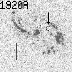
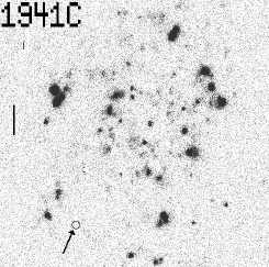
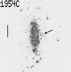
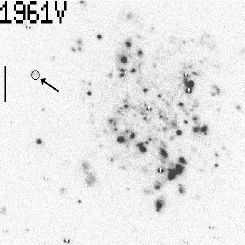
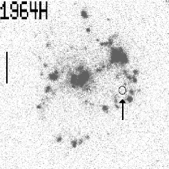
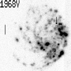
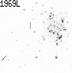
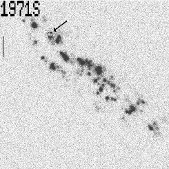
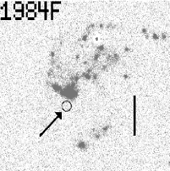
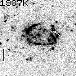
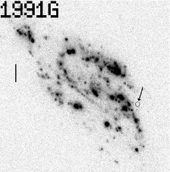
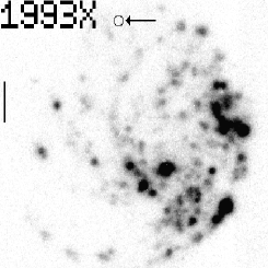
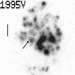
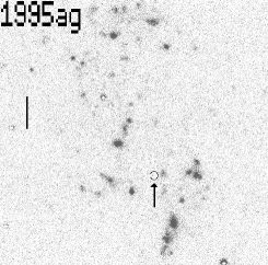
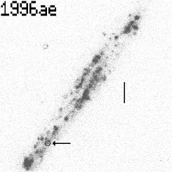
Figure 1: Positions of Type II supernovae (circles) overlaid on negative images showing the distribution of H$\alpha$$+$[Nii] emission. The scale bars are 20^′′ in length. (Continued over.)

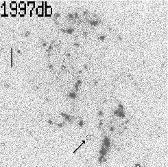
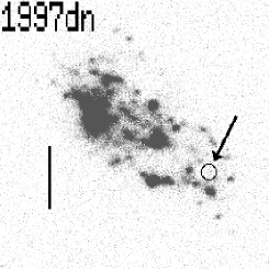
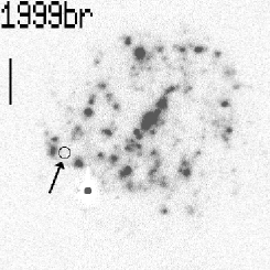
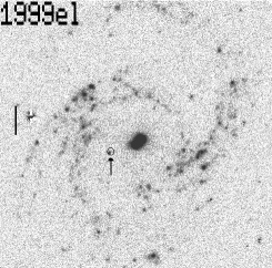
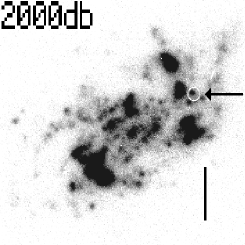
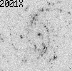
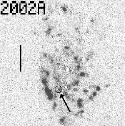
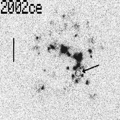
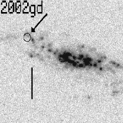
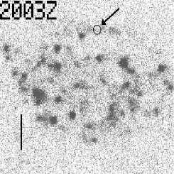
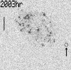
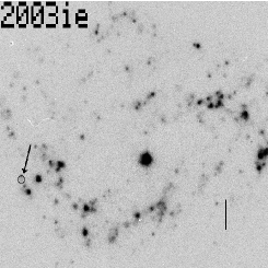
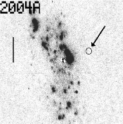
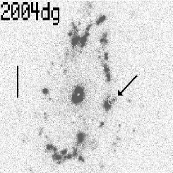
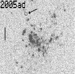
Figure 2: Positions of Type II supernovae (circles) overlaid on negative images showing the distribution of H$\alpha$$+$[Nii] emission. The scale bars are 20^′′ in length.

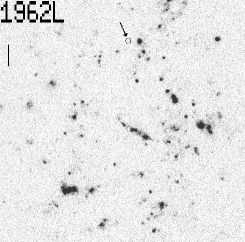
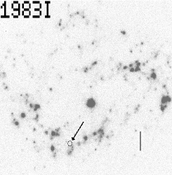
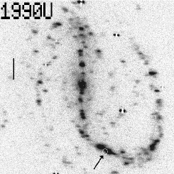
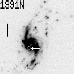
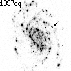
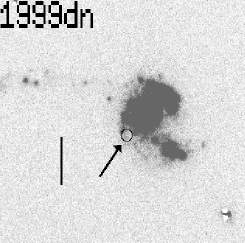
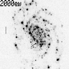
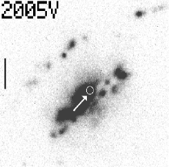
Figure 3: Positions of Type Ib and Ic supernovae (circles) overlaid on negative images showing the distribution of H$\alpha$$+$[Nii] emission. The scale bars are 20^′′ in length.

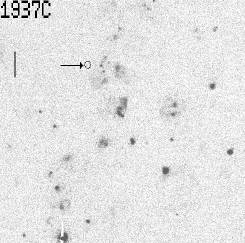
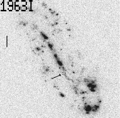
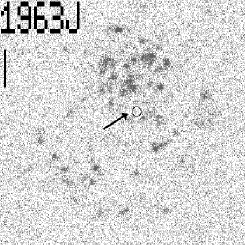
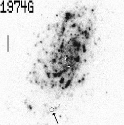
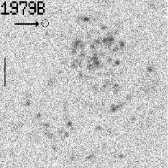
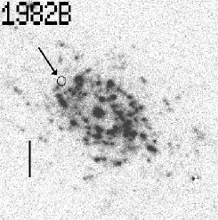
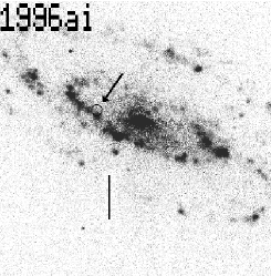
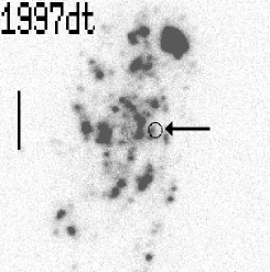
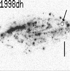
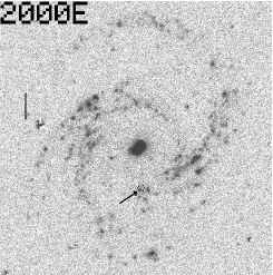
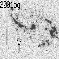
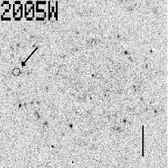
Figure 4: Positions of Type Ia supernovae (circles) overlaid on negative images showing the distribution of H$\alpha$$+$[Nii] emission. The scale bars are 20^′′ in length.

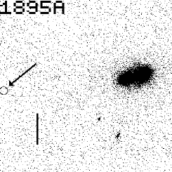
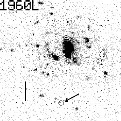
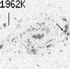
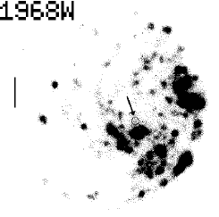
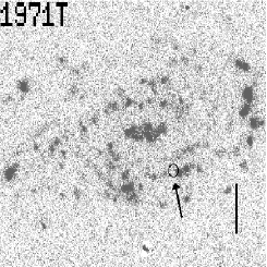
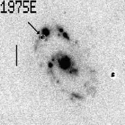
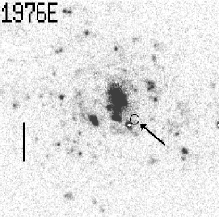
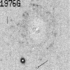
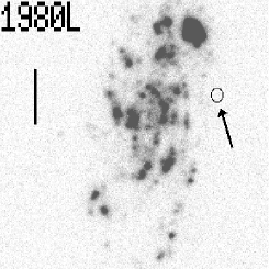
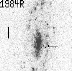
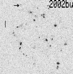
Figure 5: Positions of unclassified supernovae (circles) overlaid on negative images showing the distribution of H$\alpha$$+$[Nii] emission. The scale bars are 20^′′ in length.

4 An analysis of the SN - star formation spatial correlation based on image pixel statistics

4.1 Methods

Figures 1 and 2 show several examples where SNII are apparently strongly associated with regions of vigorous current star formation, as would be expected given the high-mass progenitors of these SNe. Examples are SN1987K, SN1999el, SN2001X, SN2002A and SN2004dg. However, there are also several apparent counter-examples, e.g. SN1941C, SN1969L, SN2003hr and SN2004A, where a SNII has occurred surprisingly far from any obvious regions of ongoing star formation, as revealed by the H$\alpha$$+$[Nii] line emission. Previous studies (e.g. Bartunov et al., 1994; van Dyk et al., 1996) have made extensive analyses of this degree of correlation or non-correlation in terms of the projected separation between each SN and the nearest prominent Hii region. It is clear from Fig. 1, however, that the morphology of star formation in galaxies does not always lend itself to the unambiguous definition of discrete regions of star formation, and many star formation regions are faint or of low surface brightness (e.g. that underlying the position of SN1961V in Fig. 1). Some fraction of the ongoing star formation must be taking place in low luminosity Hii regions and hence it is possible that the apparently ‘unassociated’ SNe could be resulting from this population. We have thus formulated the following test, based very loosely on the $V/V_{max}$ test used widely in other areas of astrophysics, which addresses this specific question: Do SNe of different types quantitatively trace the same stellar population that gives rise to H$\alpha$$+$[Nii] line emission? We test this by analysing the pixel statistics of the sky- and continuum-light-subtracted narrow-band images shown in Figs. 1–5. The images are first trimmed to the minimum size necessary to include all the line emission, plus the location of the SN, to minimise the effects of sky background uncertainty in the subsequent analysis. We then bin the pixels 3$\times$3, to reduce the pixel-to-pixel noise level and to enable us to identify with a reasonable degree of certainty the pixel containing the location of each supernova. This binning will typically result in an array of 200$\times$200 pixel values. The next stage is to sort these pixel values in order of increasing pixel count, giving a ranked sequence which starts with the most negative sky pixels and ends with the pixels from the centres of the highest surface brightness star formation regions. Alongside this ranked distribution of individual pixel values we also form the corresponding cumulative distribution, by summing the pixel counts in the ranked sequence, giving a sequence which counts up to the total emission line flux from the galaxy. We finally divide this cumulative rank sequence by the total emission line flux, and set the initial negative values of this cumulative function to zero, giving a normalised cumulative rank pixel value function (NCRPVF henceforth) running from 0 to 1, with one entry for each pixel in the input array. This is illustrated for one typical case, SN2002A in UGC 3804, in fig. 6. In this case, the 4500 ranked pixels have values from –7 to $+$52, and are plotted with larger points, which merge to give the thicker curved line running across the lower part of this plot. The cumulative pixel sum, scaled to fit on the same plot, is shown by the smaller points/thinner curved line; note how this reaches a minimum where the individual pixel values reach zero. The line to the right of the plot indicates the NCRPVF scale, which runs from where the cumulative function reaches zero (NCRPVF$=$0) up to its maximum (NCRPVF$=$1). In this case, the SN lies on a pixel with a value of 4.5 counts; reading vertically upwards to the cumulative scale and then horizontally to the NCRPVF scale indicates how the value of 0.401 is determined for this SN.

Figure 6: Illustrative example showing the calculation of the NCRPVF index for SN2002A in UGC 3804. The larger points/thicker curved line shows the ranked pixel values plotted against number in the ranked pixel sequence; the smaller points/thinner line shows the cumulative counts for each pixel, vertically scaled to fit. The pixel containing the location of SN2002A has a value of 4.5 counts, corresponding to an NCRPVF index of 0.401 as shown.

In forming the NCRPVF it is always found that a large fraction of the pixels together contribute nothing to the final flux total; these are defined as background pixels and are those for which the NCRPVF is set to zero. It is important to note that there are approximately equal numbers of positive and negative pixels contributing to this sky background region, as the cumulative function reaches a minimum when the zero value of individual pixel values is reached, and it then requires an equal number of positive pixels to bring the cumulative function back to zero. Of the remaining pixels which do contribute positive counts to the total, the majority lie close to but just above this positive sky level, but by force of numbers can contribute a significant fraction of the total flux. If the cumulative flux distribution truly represents the total star formation activity in each galaxy, and SNe of a particular type are drawn at random from this same star forming population, then SNe should be equally likely to come from any part of the NCRPVF. Thus, over a long period of time, the many pixels contributing to the 0-0.1 section of the NCRPVF contribute as much to the total star formation rate of the galaxy, and hence should host as many SNe, as the few bright pixels comprising the 0.9-1.0 section. Thus, the test we perform is to see whether the positions of the SN-containing pixels within the NCRPVF for their host galaxy are uniformly distributed between 0 and 1. Any population that is randomly scattered throughout the host galaxies and not preferentially associated with Hii regions will tend to lie at the low end of the NCRPVF, since as stated above the huge majority of pixels has low or zero values; any population purely associated with the cores of bright Hii regions will tend to lie towards the high end of the NCRPVF.

One obvious source of error in this method of calculating the NCRPVF value is uncertainty in the precise position of the SN. To quantify this error, we repeated the calculation of the NCRPVF for each SN location by replacing the exact pixel value at the SN location by the median pixel value in the 3$\times$3 pixel box centred on that location. In almost all cases this made no significant difference to the calculated NCRPVF value, and the mean value calculated using the exact location was just 0.021 larger than when using the median pixel of 9. The RMS difference in NCRPVF value was 0.128, which was dominated by two large differences of 0.555 and 0.660; with these excluded the RMS difference fell to 0.070. The two large differences are for SN1937C and SN1995ag. For both of these, the SN lies on a fairly bright pixel surrounded by 8 which are consistent with sky values. Hence these may be due to cosmic rays which have escaped detection, but since we have already binned the pixels up to 1^′′ these could be genuine small HII regions with most of their emission line flux lying in one pixel. Apart from these two cases, the NCRPVF analysis seems to give results which are robust to positional errors at the 1–2^′′ level.

A second possible source of error in the NCRPVF values is the adopted sky level in the galaxy image. This was checked by changing the sky value to extreme maximum and minimum values and recalculating the NCRPVF. However, the changes found were small, as all the pixels in the ranked distribution change together, and the only effect is on the overall flux value used to normalise the position of the SN-containing pixel in this ranked distribution.

We also performed a Monte-Carlo analysis of the effects of pixel-to-pixel noise on the NCRPVF value. This was done by adding a further noise component to each pixel of the image used to derive the NCRPVF value, including the SN-containing pixel. The added noise had a mean value of zero, and a standard deviation equal to that of a blank sky region of the same image. Thus we were effectively increasing the sky noise by a factor of 1.4 in each simulation. This was done several 10s of times for each image, with the NCRPVF value being calculated each time. The standard deviation of the simulated NCRPVF values was then taken as the error on the NCRPVF value which we quote in Table 1, i.e. the quoted error is a measure of how much the position of the SN-containing pixel shifts in the normalised distribution as a result of the extra noise being added to all pixels in the image. In general, the NCRPVF values were found to be quite robust, in particular those from the extremes of the distribution. A few cases were found (SN1937C, SN1962K, SN1995ag and SN2002A; note that two of these were also found to be sensitive to positional error effects above) where this addition of noise can significantly affect the derived value, but omission of these has no effect on the conclusions presented here. This also appears to be a random effect, with no tendency to bias the results in one particular direction.

The NCRPVF analysis can also be applied to our $R$-band images of these galaxies, but in this case the method produces very similar results to the much simpler process of comparing supernova locations with the radial growth curve of the galaxy light, which we discuss in the next section. This is because the brightest pixels in the $R$-band always occur in the galaxy nucleus, and the ranked squence thus runs monotonically from the outer regions of the galaxy into the nucleus. Thus, the $R$-band equivalents of figs. 7 and 8 are essentially identical to figs. 9(b) and 10(b), which are explained in section 5.

The value for each SN-containing pixel within its host galaxy NCRPVF is listed in col. 7 of Table 1. We will next discuss the distributions of these values for the different types of SNe.

4.2 Core-collapse supernovae

Figure 7 shows the distribution of NCRPVF values for the 30 SNII in the current sample (solid histogram), and the dashed line indicates the distribution of all core-collapse SNe, i.e. including the 8 SNIb, Ic and Ib/c (SNIbc henceforth). It is immediately clear that neither of these distributions is flat, with the majority of these supernovae having low NCRPVF values, corresponding to regions of no or low surface brightness line emission. The mean NCRPVF value for the 30 SNII is 0.274 with a standard error on the mean of 0.053, while for all 38 core-collapse SNe the mean is 0.320, standard error 0.051. These distributions are confirmed by a Kolmogorov-Smirnov (KS) test to be inconsistent with a flat distribution, at the $<1\%$ level. The excess is concentrated in the two bins below 0.2, with 18 of the 30 SNII having values below this limit, compared with an expectation value of 6 if the SNII came from a parent population traced by the line emission. Thus the excess of low NCRPVF values is 12, or 40% of the total. For the 8 SNIbc considered alone, the conclusion is very different, with these having a mean NCRPVF value of 0.490, standard error 0.121, and being formally consistent with having been drawn from a flat parent distribution, as confirmed by a KS test. Hence the latter types are consistent with being distributed evenly over the NCRPVF range of 0–1, and these SNe do seem to follow the same spatial distribution as the line emission in their host galaxies, although the uncertainties are great as a result of the small sample size. It is noteworthy that 2 of the 3 highest NCRPVF values, and 4 of the 9 highest values, are found for SNIbc, which only comprise 8 out of 63 SNe in the full sample. Thus the SNIbc seem more likely than SNe of any other type to lie close to the centres of luminous Hii regions, as would be expected for SNe with the highest-mass progenitor stars.

Figure 7: Histograms of the positions of the SN-containing pixels within the cumulative H$\alpha$$+$[Nii] flux distributions for the 30 Type II supernovae (solid line); and for all 38 core-collapse supernovae (dashed line).

4.3 SNIa

Figure 8 shows the distribution of NCRPVF values for the 12 SNIa. As expected, this distribution is strongly weighted towards low values, with a mean value of 0.188 and a standard error on the mean of 0.069. Again, a KS test shows $<$1% chance of these values having been drawn from a flat parent distribution, and indeed the SNIa appear even more weakly correlated with line emission than the SNII. It is natural to ask whether there is any correlation at all between the locations of SNIa and the sites of active star formation, or whether the distribution of values in Fig. 8 is consistent with that expected for random locations within the host galaxies. A simple test was performed to address this question, by comparing the SN-containing pixel value with the median pixel value over the subset image used for the NCRPVF calculation. Clearly, pixels chosen completely at random from these images would be equally likely to lie above or below this median value, by definition. It was found the 8 of the SNIa locations had pixel values above the median, and 4 below, showing a weak correlation between SNIa and ongoing star formation. It can also be argued, however, that this correlation could reflect the concentration of all stellar populations towards the centres of host galaxies, and may not imply any causal link.

Figure 8: Histogram of the positions of the SN-containing pixels within the cumulative H$\alpha$$+$[Nii] flux distributions for the 12 Type Ia supernovae (solid line).

4.4 The full sample, and unclassified SNe

We also looked at the distribution of NCRPVF values for all 63 SNe in the current sample, and for the 13 unclassified SNe. Again a strong tendency was found for most NCRPVF values to be low, with a mean value of 0.285, standard error 0.036 for the full sample. The unclassified SNe have a mean NCRPVF value of 0.272, standard error 0.063, and hence are completely consistent with being drawn at random from the overall population of SNe. This indicates that no strong biases should be caused by the incompleteness of type information; whatever the types of the unclassified SNe, their inclusion in Figs. 7 and 8 would have little or no effect on our conclusions.

5 Study of the radial distribution of SNe locations, relative to SF and $R$-band light in host galaxies

5.1 Methods

In this section we perform a statistical test related to that in the previous section, but in this case specifically to determine whether the radial locations of SNe within their host galaxies are consistent with their being drawn at random from the star-forming population traced by H$\alpha$$+$[Nii] emission, or the older stellar population traced by $R$-band emission. The data for this test were the H$\alpha$$+$[Nii] and $R$-band growth curves which were determined for all H$\alpha$GS galaxies using methods described in Paper I. Briefly, these curves were derived using elliptical apertures with fixed centres, ellipticities and position angles, with values for the ellipse parameters being taken from the UGC. For each SN, we then calculated the size of the elliptical aperture of the same shape and orientation as its host galaxy which just included the location of the SN, and thus were immediately able to calculate the fraction of both H$\alpha$$+$[Nii] and $R$-band light lying inside and outside the SN location, by reference to the equivalent points on the growth curves. If, for example, the core-collapse SNe are equally likely to come from any part of the star-forming population of their host galaxies, we would expect the fractions of H$\alpha$$+$[Nii] light within the SN locations to be evenly distributed between 0 and 1, with an average of 0.5 (note that throughout this analysis we quote the fractions within the SN location, i.e. closer to the galaxy nucleus). This is the test we present in this section, splitting the SNe into types II, all CC and Ia in turn, and testing all three categories against both the H$\alpha$$+$[Nii] and $R$-band light distributions of their host galaxies. We also look briefly at the properties of the unclassified SNe, and of the total sample of 63 SNe.

5.2 Core-collapse supernovae

The solid line in Fig. 9(a) shows the distributions of fractions of H$\alpha$$+$[Nii] emission coming from regions lying within the locations of the SNe, for the host galaxies of the 30 SNII in the present study. The dashed line shows the same data, but with the addition of the 8 SNIbc. Overall, both histograms are close to the flat distributions expected if these SNe perfectly trace the young line-emitting stellar population. The only deviation from a completely flat distribution is the deficit in SNe arising from the very central parts of the H$\alpha$$+$[Nii] distribution. Note that, because the H$\alpha$$+$[Nii] emission can exhibit significant central holes e.g. in galaxies with purely old stellar bulges, a SN can in some cases lie some distance from the physical centre of its host galaxy and still be at the centre of the distribution of line emission in Fig. 9(a). This departure from flat distributions was shown by a KS test to be marginally significant, at the 0.10 level. There is a slight tendency for the SNIbc to lie closer to the centres of their host galaxies than the SNII, with the mean fractions of SF lying within the SN locations being 0.612$\pm$0.045 for the SNe II, against 0.446$\pm$0.088 for the SNIbc. This difference is of marginal statistical significance (1.7$\sigma$), but was also found by van den Bergh (1997) for a rather larger sample (16 SNIbc and 58 SNe II), and it is noteworthy that, in the current study, the two lowest fractions in Fig. 9(a) correspond to SNIbc, SN2005V and SN2000ew. This provides some support for the suggestion of metallicity being linked to the difference between these SNII and SNIbc (discussed in van den Bergh, 1997).

Two explanations can be suggested for the apparent central deficit in CC SNe. The first and probably dominant effect is the systematic failure to detect SNe in the central regions of galaxies due to either the high surface brightness of the stellar background (Shaw, 1979) or extinction effects which have been deduced to result in significant deficits in SN detection rates, even in near-IR searches (Mannucci et al., 2003). The second possible explanation is that there is an additional emission-line component at the centres of these galaxies which is not related to star formation, and hence not linked to CC SNe. Such a component could be related to AGN (although most of these galaxies do not show strong unresolved central emission-line sources) or to the extended nuclear emission-line sources noted by Hameed & Devereux (1999) and James et al. (2005). If such a component were to lie predominantly inside the innermost star formation regions, it could contribute to the central drops in the histograms shown in Fig. 9.

We also note that the central deficit in SN numbers appears much larger when the SNII distribution is compared with the $R$-band light distribution (Fig. 9(b)). In this case, none of the SNe lies within the central 30% of the light distributions of their host galaxies, and the difference from a flat distribution is now quite significant, at the 0.01 level. This greater deficit is simply explained as being due to the central older bulge population with no associated SNII.

Figure 9: (a) Histograms of fractional H$\alpha$$+$[Nii] fluxes within the locations of 30 Type II supernovae (solid line); and all 38 core-collapse supernovae (dashed line). (b) Histograms of fractional $R$-band fluxes within the locations of 30 Type II supernovae (solid line); and all 38 core-collapse supernovae (dashed line).

5.3 SNIa

Figure 10 shows the comparison of the positions of the 12 SNIa relative to the H$\alpha$$+$[Nii] and $R$-band light distributions of their host galaxies. With the low-number statistics, both histograms are formally consistent with flat distributions, and it is impossible to determine from these data whether SNIa better trace the young or old stellar populations. The SNIa appear more centrally-concentrated than the type II or CC SNe, with no evidence for a central deficit in either Figs. 10 (a) or (b).

Figure 10: Histogram of (a) fractional H$\alpha$$+$[Nii] fluxes, and (b) fractional $R$-band fluxes, within the locations of the 12 Type Ia supernovae

5.4 Unclassified supernovae

We also looked briefly at the distributions of fractions of SF and of $R$-band light within the locations of all 63 SNe in the present study, and compared these with the values for the 13 unclassified SNe. The central deficits noted for the CC SNe persist when the full sample is considered, with mean fractions of 0.560$\pm$0.03 relative to the SF distribution and 0.584$\pm$0.033 relative to the $R$-band light distribution. The unclassified SNe have distributions consistent with their being drawn at random from the full distribution of 63 SNe.

6 Comparison of galactic supernova rates and host galaxy star formation rates

6.1 Methods

In this section, we perform a test of whether the frequency of occurrence of SNe within galaxies appears to scale with their total star formation rates, as revealed by H$\alpha$$+$[Nii] fluxes, or with their $R$-band luminosities. One motivation for this test is the suspicion that lower-luminosity galaxies may be less intensively studied than their more spectacular counterparts, resulting in a larger fraction of their SNe being missed entirely. The test is in some ways analogous to that performed with respect to light distributions within individual galaxies, but here the test is performed on the whole ensemble of H$\alpha$GS galaxies, since the probability of a detected supernova in any one of the galaxies is small. The only data used are the total H$\alpha$$+$[Nii] fluxes (or equivalently total star formation rates, where we use the conversion formula of Kennicutt (1998)) and total $R$-band luminosities of each of the 327 H$\alpha$GS UGC galaxies. These total fluxes were sorted into ranked sequences, running from the lowest intrinsic luminosity of the 327 up to the highest, and were then summed in that order to construct cumulative luminosity distributions in both H$\alpha$$+$[Nii] and $R$-band light. These were then normalised by the total luminosity in each band for all 327 galaxies, to give cumulative distributions running from 0 to 1. We then tested to see where in these normalised cumulative distributions lay the galaxies hosting the SNe of the different types already discussed in this paper, and performed K-S tests to see whether they were biased towards galaxies of high or low star formation rates or luminosities.

Note that there is no assumption in this test that the H$\alpha$GS sample in any sense constitutes a statistically complete sample of galaxies. Although it is representative of the star-forming galaxies in the UGC, the magnitude and diameter selection criteria necessarily lead to the very faintest and smallest galaxies being under-represented relative to a truly volume-limited sample. The question is simply whether, for a given sample of galaxies selected in a way which is hopefully unbiassed with respect to the likelihood of SNe occurring in particular galaxies, the probability of a SN being detected in a particular galaxy within that sample depends linearly on its current star formation rate or $R$-band luminosity.

6.2 Core collapse SNe

As the first example of this test, the solid line in Fig.11 (a) shows the distribution of the locations of the host galaxies of the 30 SNII in the ranked, cumulative H$\alpha$$+$[Nii] distribution for the H$\alpha$GS galaxy sample (solid line). The dashed line shows the effect of adding in the 8 SNIbc to give the distribution for all core-collapse SNe. The distribution for SNII is close to flat, but contrary to our expectations it shows a marginal deficit in SNII within the galaxies with the highest star formation rates (shown by the lack of points above 0.8 in the cumulative distribution). The mean value for all 30 SNII is 0.435$\pm$0.047, reflecting this marginally significant deficit at the high star formation rate end. A KS test gives a 20% chance that these values could have been drawn from a flat distribution. The 8 SNIbc, on the other hand, seem to come preferentially from galaxies with high star formation rates, with a mean value of 0.651$\pm$0.087, higher than that for the SNII with a significance of just over 2$\sigma$. For all core collapse SNe combined together, the distribution is statistically completely flat, with a mean value of 0.481$\pm$0.044. Thus it would appear that galaxies with low star formation rates contribute at least their expected numbers of core collapse SNe, and there is no evidence for the expected selection bias against detecting SNe in such galaxies.

Figure 11 (b) shows the test for the same SN host galaxies, against the ranked cumulative distribution of $R$-band luminosities of the 327 H$\alpha$ GS galaxies. Here again a tendency is seen for the SNII (solid histogram) to come preferentially from the fainter galaxies, with the mean location of the SNII-hosting galaxies within the overall distribution being 0.367$\pm$0.053. A KS test gives only a 5% probability that these values are consistent with a flat parent distribution. The SNIbc values (the difference between the dashed and solid histograms) are consistent with an unbiased distribution with respect to galaxy $R$-band luminosity (mean 0.531$\pm$0.077), and the mean value for the galaxies hosting all 38 core-collapse SNe is 0.409$\pm$0.046.

Figure 11: (a) Histograms of the locations of galaxies in the ranked cumulative H$\alpha$$+$[Nii] distributions for 30 type II supernovae (solid line) ; and all 38 core-collapse supernovae (dashed line). (b) Histograms of the locations of galaxies in the ranked cumulative $R$-band luminosity distributions for 30 type II supernovae (solid line); and all 38 core-collapse supernovae (dashed line).

6.3 SNIa

Figure 12 (a) shows the distribution of the SNIa-hosting galaxies in the cumulative galaxy star formation distribution, and displays a slight bias towards low values (mean 0.361$\pm$0.085, KS significance 0.20). Figure 12 (b) shows the equivalent values within the cumulative $R$-band light distribution, which is formally consistent with a flat distribution (mean 0.462$\pm$0.100). Thus, as far as can be deduced from such small numbers, the SNIa rates seem to scale with the $R$-band luminosities of their host galaxies, and there is again no evidence of any selection-induced deficit in SN numbers from low-luminosity galaxies. $R$-band luminosity appears a better predictor of SNIa rates in these galaxies than star formation rate.

Figure 12: Histogram of the locations of the galaxies hosting the 12 Type Ia supernovae in (a) the ranked cumulative H$\alpha$$+$[Nii] distribution and (b) the ranked cumulative $R$-band light distribution.

6.4 All and unclassified SNe

We repeated this analysis for the positions of all 63 SN-hosting galaxies within the total star formation distribution and within the total $R$-band light distribution. Both tests show a small bias towards low values (means 0.444$\pm$0.038 and 0.437$\pm$0.038 respectively), again showing that there is no evidence for selection biases against low-luminosity galaxies. The values for galaxies hosting unclassified SNe are again completely consistent with being drawn at random from the overall SN population analysed here.

The main conclusions from this section are that the SNIbc are the only types which may preferentially occur in larger galaxies, and particularly in those with high star formation rates, although this is only of marginal significance due to the small number of SNIbc in our sample. Other types of SNe show a slight tendency to occur preferentially in fainter galaxies, and those with lower star formation rates. This second result also suffers from low number statistics, but if true it is somewhat surprising. One possible explanation is that SN detection rates are higher in low luminosity galaxies due to smaller dust extinction, although this explanation would require dust to have a larger effect on SN rates than on emission of $R$-band and H$\alpha$ photons. This extinction dependence is consistent with the interpretation of SN detection rates in the near-IR in the study by Mannucci et al. (2003).

Figure 13: (a) Histograms of the locations of galaxies in the ranked cumulative H$\alpha$$+$[Nii] distributions for all 63 supernovae in the present study (solid line); and for the 13 unclassified supernovae (dashed line). (b) Histograms of the locations of galaxies in the ranked cumulative $R$-band luminosity distributions for all 63 supernovae in the present study (solid line); and for the 13 unclassified supernovae (dashed line).

7 Discussion

The most interesting result from this analysis is probably the finding that many of the SNII in the current sample have no associated ongoing star formation, as indicated by H$\alpha$ $+$ [Nii] line emission. This has also been found by previous authors, e.g. van Dyk (1992), van Dyk et al. (1996) and Bartunov et al. (1994), and the significance of the present result has been strengthened by the statistical analysis presented in section 4. This analysis shows that there is a real excess, of $\sim$40% of the total, of SNII in regions of zero or low line flux, compared to what is expected if line emission accurately traces high-mass star formation. We will briefly discuss two alternative (but not mutually exclusive) explanations for this result.

The first possibility is that each SNII progenitor did indeed form in an HII region in the location indicated by the currently-measured line emission, and then moved out of the HII region between birth and death. We estimate an upper limit for the time available for this process from the lifetime of a 10 M_⊙ star, which current stellar models put at 2.2$\times$10⁷ years, independent of metallicity to a good approximation. As an illustrative calculation, we have derived the component of velocity of the plane of the sky required for some of the most anomalous SNII progenitors to have moved to the location where the SN was observed, from the nearest bright HII region. We have done this for the 7 SNII with NCRPVF values of 0.000 in Table 1, i.e. those which appear to have no associated line emission. We use the galaxy distances listed in Paper I. The results are listed in Table 2, where col. 1 gives the SN name, col. 2 the host galaxy UGC number, col. 3 the galaxy distance in Mpc, col. 4 the projected angular distance from the SN to the centre of the nearest bright HII region, in seconds of arc, col. 5 the same projected distance in kpc, and col. 6 the lower limit on the estimated progenitor velocity.

SN	UGC	D(Mpc)	Rp(′′)	Rp(kpc)	V⋆(km s-1)
2005ad	1954	18.1	10.2	0.90	41
2004A	10521	15.0	10.9	0.79	36
2003hr	4362	33.1	20.2	3.24	147
2003Z	4779	21.3	9.5	0.98	45
1969L	2193	6.9	102.0	3.41	155
1941C	7634	6.8	18.5	0.61	28
1920A	4484	32.1	7.2	1.12	51

Table 2: Distance and drift velocity data for SNII with no associated line emission.

The required velocity components of the progenitor stars are between 28 and 155 km s^-1, with a median of 45 km s^-1. These values are very comparable to those attributed to the OB runaway stars, which are traditionally defined as having a minimum peculiar velocity of 40 km s^-1 (Blaauw, 1961), and may reach values as large as 200 km s^-1 (Dray et al., 2005). The fraction of OB stars that are runaways has been estimated at between 7% and 49% (Gies & Bolton, 1986, and refererences therein). Thus the estimated 40% excess of SNII lying away from regions of present star formation could be explained by the runaway phenomenon, but the fraction is uncomfortably large and certainly lies at the upper end of the frequency of stars previously thought to be affected by this phenomenon. It would also seem impossible to explain such a high fraction of runaway stars through the binary-binary encounter mechanism first proposed by Poveda et al. (1967), which ejects only one of the four massive stars involved in the ejection mechanism, whereas the binary supernova hypothesis of Blaauw (1961) could presumably result in up to 50% of massive stars being ejected from the star formation region where they formed, and hence may be consistent with our findings.

An alternative explanation is that H$\alpha$ line emission is not a good tracer of all star formation, and that $\sim$40% of all star formation takes place in locations from which little or no line emission is produced, even though high mass stars are being produced. This could occur if the star formation process is both rapid and efficient, depleting the gas reservoir so that no detectable ionized gas remains when SNe occur. Alternatively, the dust geometry might be such that the ionized gas is not visible, even though the SNe are visible.

Due to the small number of SNIa in the present sample, it is hard to draw any firm quantitative conclusions from these observations. It is, however, of interest to consider the environments of these 12 SNIa in light of recent suggestions that there may be two populations of SNIa, with ‘prompt’ SNIa occurring shortly after the formation of their parent stellar population, and ‘delayed’ SNIa occurring when the stellar population is typically some Gyr old (Mannucci et al., 2005). The pixel analysis of the locations of SNIa relative to H$\alpha$ emission showed clearly and unsurprisingly that these SNe as a whole do not trace the young stellar population in their host galaxy, and 7 of the 12 (58%) have NCRPVF values consistent with coming from background regions with no ongoing star formation. These 7 are most likely to be associated with the ‘delayed’ fraction of SNIa. The remaining 5 (42%) generally show good degrees of correlation with sites of active star formation, and it is tempting to ascribe these to the ‘prompt’ fraction of SNIa. However, it should be remembered that some of these may be coincidental alignments of intrinsically old systems with regions of the galaxy undergoing later bursts of star formation, so the number of true ‘prompt’ SNIa may be smaller than 5, and comparison of figs. 8 and 10(b) demonstrates that overall the SNIa more closely follow the older stellar population traced by $R$-band light than they do the extremely young stars traced by H$\alpha$. Thus, with the current data we cannot exclude the possibility that all SNIa come from an old stellar population, but our preferred conclusion is that while the majority seem to be linked to the old stellar population, a significant minority ($\leq$42%) are linked to regions of ongoing star formation.

8 Conclusions

• From a pixel statistics analysis, we find an excess of SNII coming from regions of no or weak star formation activity, as traced by H$\alpha$ line emission.

• SNIbc do appear to trace star formation activity, with many of them coming from the centres of bright star formation regions.

• SNIa are only marginally more likely to be found towards star formation regions than would be expected by chance, but our data are consistent with a significant minority, $\leq$42%, being associated with ongoing star formation.

• The radial distribution of CC SNe closely follows that of the H$\alpha$ line emission.

• We find a lack of SNII from central regions of their host galaxies, possibly due to a component of the line emission not associated with SF; alternative explanations include extinction effects, or SN missed in high SB regions even in nearby galaxies.

• There is some evidence that SNIbc are more centrally concentrated than SNII, possibly indicating that the former preferentially occur in high metallicity regions

• Overall, detected CC SN rates scale approximately linearly with both their host galaxy luminosities and star formation rates. However, relative to this overall trend, the SNII show a weak bias towards low-luminosity (and star formation rate) galaxies, and the SNIbc towards high-luminosity (and star formation rate) galaxies.

• SNIa rates scale more closely with galaxy $R$-band luminosity than with star formation rates.