The variable X-ray light curve of GRB 050713A: the case of refreshed shocks.

We present a detailed study of the spectral and temporal properties of the X-ray and optical emission of GRB050713a up to 0.5 day after the main GRB event. The X-ray light curve exhibits large amplitude variations with several rebrightenings superposed on the underlying three-segment broken powerlaw that is often seen in Swift GRBs. Our time-resolved spectral analysis supports the interpretation of a long-lived central engine, with rebrightenings consistent with energy injection in refreshed shocks as slower shells generated in the central engine prompt phase catch up with the afterglow shock at later times. Our sparsely-sampled light curve of the optical afterglow can be fitted with a single power law without large flares. The optical decay index appears flatter than the X-ray one, especially at later times.

1 Introduction

A commonly accepted wisdom in the pre-Swift era was that the optical and X-ray afterglows of Gamma Ray Bursts (GRBs) showed a smooth power law decay with time after the burst (e.g. Laursen & Stanek 2003). This behavior was found to be consistent with the fireball model, where the afterglow flux is produced when a relativistic blast wave propagating into an external medium. Under the assumption of a spherical fireball and a uniform medium, Sari, Piran & Narayan (1998) showed that the dependence of the flux on frequency and time can be represented by several power law segments, $F_{\nu}\propto\nu^{-\beta}t^{-\alpha}$. Before Swift only a few GRBs showing deviations from the smooth power law light curve were known, see e.g. the case of GRB 021004 (Bersier et al. 2002; Matheson et al. 2002). Its lightcurve was densely sampled in the optical, allowing detailed modeling. The bumps were interpreted as due to overdensities in the interstellar medium in which the afterglow is produced (Lazzati et al. 2002; Nakar et al. 2003; Heyl & Perna 2003). On the other hand, Bjornsson et al. (2004), Nakar et al. (2003) and de Ugarte Postigo et al. (2005) modeled these fluctuations as due to several energy injection episodes. Several re-brightenings were observed also in the optical light curve of GRB 030329 and were interpreted as due to refreshed shocks (Granot, Nakar & Piran 2003, Huang et al. 2006).

This simple picture is now changing since the advent of Swift. Bright X-ray flares have been recently observed by Swift in almost half of its detected GRBs (Gehrels et al. 2005; Burrows et al. 2005b; Falcone et al. 2006; Nousek et al. 2005; O’Brien et al. 2006). While some bursts show one distinct flare, like GRB 050406 (Romano et al. 2006), other events like GRB 050502B and GRB 050713A show several flares (Burrows et al. 2005; O’ Brien et al. 2006; Falcone et al. 2006). One of the main current goals of the GRB community is to understand the origin of this newly observed light curve behaviour. Since flares are likely to trace the activity of the internal engine, they can help us gain a more comprehensive view of the physical processes governing the early phases of GRB activity. Flares have been observed in the light curves of both long and short GRBs. For the long bursts, King et al. (2005) proposed a model in which the flares could be produced from the fragmentation of the collapsing stellar core in a modified hypernova scenario. For the case of short GRBs, MacFadyen et al. (2005) suggested that the flares could be the result of the interaction between the GRB outflow and a non-stellar companion. More recently, Perna et al. (2006) have analyzed the observational properties of flares in both long and short bursts, and suggested a common scenario in which flares are powered by the late-time accretion of fragments of material produced in the gravitationally unstable outer parts of the hyperaccreting accretion disk. Other mechanisms that could produce flares are of magnetic origin (Gao et al. 2005; Proga & Zhang 2006). In this paper we concentrate on one particular burst that presents flaring activity, GRB 050713A, and perform a detailed spectral and timing analysis of its main flare with the goal of constraining the physical mechanisms that can be responsible for its production.

The Swift BAT localized this burst on 2005, July 13.1866 UT to a 3′ radius error circle (Falcone et al. 2005). The BAT light curve is characterized by a main event lasting $\sim 13sec$ that drops by a factor of 100, followed by two rebrightenings starting $\sim 53$ s and $\sim 110$ s after a time $t_{0}$ s, that corresponds to the time at which BAT started to detect the burst. The spectrum of the main event could be fitted with a power law with energy index $0.58\pm 0.07$, yielding a fluence of $(9.1\pm 0.6)\times 10^{-6}$ erg cm^-2 (15–350 keV). The peak flux in 1 s window time is $6.0\pm 0.4$ ph cm^-2 s^-1 (Golenetskii et al. 2005). Swift slewed promptly toward the position of the GRB and XRT started to observe this event just 70 s after the trigger. The XRT light curve was dominated by a major rebrigthening event 117 s after $t_{0}$, nearly coincident with the second rebrightening detected by BAT. Both the 15–350 keV and the 0.5–10 keV fluxes varied up and down by a factor of $\sim 10$ in about 40 s. A second XRT rebrightening event occurred about 186 s after the $t_{0}$, and other smaller amplitude flares were seen at later times (around $\sim 10^{4}$ s). In this paper we focus on the first major XRT rebrightening event through both a temporal and a time-resolved spectral analysis. The statistics of the spectra of the second flare are not good enough to allow a similar detailed analysis. Furthermore, we use XMM-Newton data to better constrain the late time afterlow decay.

We show that the rebrightening in the early-time afterglow light curve is consistent with energy “injections”, probably due to later shells that catch up with the main shock at later times.

The redshift of GRB 050713A is not known. The host galaxy is not detected, and the limit on its magnitude is quite shallow ($R{{}_{<}\atop{}^{\sim}}23$), due to the high background caused by a nearby ($\sim 1$ arcmin), bright star.

2 Observations and data reduction

2.1 Swift XRT observations

XRT started observing GRB050713A at 2005-07-13, 04:30:14.9, just 70 s after the BAT trigger. The observation lasted until 2005-07-13, 08:50:27 (UT), for a total of $\sim 1700$ s net integration time. Within this observation, XRT observed the GRB in three consecutive orbits.

The data were reduced using the Swift Software (v. 2.0) and in particular the XRT software developed at the ASDC and HEASARC (Capalbi et al. 2005). Standard screening criteria were adopted to reject “bad” events following Capalbi et al. (2005). In particular, the constraint on the angular distance between the source position and the satellite position (which must be less than $0.08$ deg, Capalbi et al. 2005), led us to exclude the first part of the first orbit and 80% of the last orbit. The GRB was observed by the XRT in two observing modes. During the first satellite orbit the GRB was mostly observed in windowed timing mode (WT mode, providing 1D imaging). We report here the WT data only for this orbit. During the second and third orbits the GRB was mostly observed in photon counting mode (PC mode, providing the usual 2D imaging). We report here the PC data only for these orbits. We used a $0-12$ grade selection for the PC mode and $0-2$ for the WT mode. We excluded all the events with energy below $0.3$ keV, to minimize the background due to the bright Earth limb and and because the calibration of the data below 0.3 keV are still uncertain. The intensity of the source was high enough to cause significant pileup in the PC mode. In order to avoid this pileup we extracted counts from an annulus with inner radius of $6$ pixels and outer radius of $20$ pixels (14 and 47 arcsec, respectively). We then corrected the observed count rate for the fraction of the XRT Point Spread Function (PSF) lying outside the extraction region. The correction was equal to a factor of 3.33 (i.e. 30% of the PSF lying inside the annulus). Data in WT mode were not affected by pileup and therefore we extracted counts from a circular region of $20$ pixels radius (47 arcsec). Physical ancillary response files were generated with the task xrtmkarf to account for the different extraction regions. For the spectral fits we used the latest redistribution matrices (version 7).

2.2 XMM-Newton observations

XMM-Newton (Jansen et al. 2001) observed this GRB for about 30 ks starting from 2005-07-13 10:18 UT, about six hours after the trigger, observation ID 0164571001 (Loiseau et al. 2005). The data were processed using the XMM-Newton Science Analysis Survey (SAS) v.6.1.0. We used the raw event files (i.e. the observation data files, ODF), which were linearized with the XMM-SAS pipelines, epchain and emchain for the PN (Strűder et al. 2001) and MOS (Turner et al. 2001) cameras respectively. Events spread at most in two contiguous pixels for the PN (i.e. grade=0–4) and in four contiguous pixels for the MOS (i.e, grade=0–12) have been selected. Event files were cleaned from bad pixels (hot pixels, events out of the field of view, etc.). In order to remove periods of high background, we analyzed the light curves of the counts from the entire EPIC PN and MOS CCDs at energies higher than 10 keV, where the X-ray sources contribution is negligible. We rejected time intervals, in which this count rate was higher than 10 counts s^-1 and 1.5 counts s^-1 for the PN and MOS cameras respectively. This corresponds to rejecting 27% (15%) of the PN (MOS) on source time. The source counts were extracted from a circular region of 47 arcsec radius (12 pixels). The background counts were extracted from the nearest source free region. The response and ancillary files were generated by the XMM-SAS tasks, rmfgen and arfgen respectively.

3 Optical observations

Figure 1: The BAT XRT and XMM-Newton PN light curve of GRB 050713A and its afterglow (solid line and points with errors). The BAT 15–300 keV count rate, the XRT and PN 0.5–10 keV count rates are converted to a flux at 1 keV assuming a power law spectrum with average spectral indices $\beta=0.5$ (BAT) and $\beta=1$ (XRT, XMM). Filled circles are the optical observations performed with the RAPTOR-S, Liverpool 2-m, TNG and NOT telescopes. The dashed line is the best fit power law decay of the optical data.

UVOT started observing the field at the same time of XRT (75 seconds after the BAT trigger) but did not detect any new source in the XRT error circle, with a 3$\sigma$ upper limit of V$\sim 18$. Shortly after the receipt of the alert, we started observing the GRB location in order to look for an optical counterpart. Observations were conducted using the Liverpool Telescope (LT), the Telescopio Nazionale Galileo (TNG), and the Nordic Optical Telescope (NOT), all located in the Canary Islands. A bright object was discovered inside the XRT error circle by inspecting the TNG $I$-band images, taken 50 min after the GRB, and was proposed as the GRB afterglow (Malesani et al. 2005). Its coordinates were $\alpha_{\rm J2000}=21:22:09.57$, $\delta_{\rm J2000}=+77:04:29.4$ (0.15″ uncertainty). Hearty et al. (2005) subsequently reported variability for this source, confirming that it was the GRB counterpart. The robotic 2-m Liverpool telescope imaged the GRB field starting from 150 seconds after the burst, detecting the afterglow in the $r\arcmin$ band (Monfardini et al. 2005). Further imaging was secured at the NOT in the $R$ band (Jul 13; Guzly et al. 2005) and at the TNG in the $I$ band (Jul 14). Only an upper limit could be obtained at the Observatorio de la Sierra Nevada (OSN) during the night of Jul 13. Unfortunately, the GRB position was close ($\approx 1\arcmin$) to a bright foreground star ($R\sim 6.5$), which caused a bright sky level, so that no further detection was possible in the following nights.

The TNG and NOT data analysis and reduction were carried out following the standard procedures. The LT data analysis was performed using the dedicated LT pipeline (Guidorzi et al. 2006). Magnitudes were computed using the SExtractor (Bertin & Arnouts 1996) and Gaia software packages. Photometric calibration was obtained by observing standard fields at the TNG ($I$ band) and OSN ($R$ band). The zeropoint, however, was computed at only one epoch, so it may suffer from systematic uncertainty. LT data were calibrated via Landolt standards with SDSS calibration (Smith et al. 2002). We combined all our data, and included the early RAPTOR $R$-band detection (Wren et al. 2005). A log of all optical observations is given in Table 1.

Figure 1 shows the light curve of the optical flux at 7000Å obtained by converting the observed R, r’ and I magnitudes into flux at 7000Åassuming a power law with spectral index of -1. Considering a power law flux decay $F(t)\propto t^{-\alpha}$, we found $\alpha=0.67\pm 0.05$. We note that, to within the limitations of the sampling, the optical light curve appears fairly smooth, with no signs of the large fluctuations seen in the X-ray region. However, the coverage is quite scarse, so that no strong conclusion can be drawn.

Table 1: Log of Optical observations

Mean time	Time since GRB	Exposure time	Instrument	Filter	Magnitude	Flux
(UT)	(s)	(s)				($\mu$Jy)
13.18709	99.3	8$\times$10	RAPTOR	$R$	18.4$\pm$0.18	125$\pm$25
13.22112	2963	1$\times$180	NOT+ALFOSC	$R$	21.41$\pm$0.08	8.4$\pm$0.7
13.22484	3284	1$\times$180	NOT+ALFOSC	$R$	21.37$\pm$0.12	8.7$\pm$1.0
13.22930	3670	3$\times$60	NOT+ALFOSC	$R$	21.44$\pm$0.20	8.2$\pm$1.6
14.08340	77468	1$\times$3900	OSN+CCD	$R$	$>$22.50	$<$3.1
13.18872	150	10	LT+RATCAM	$r\arcmin$	19.25$\pm$0.14	72.4$\pm$9.3
13.18896	171	10	LT+RATCAM	$r\arcmin$	19.45$\pm$0.17	60.3$\pm$9.4
13.18920	192	10	LT+RATCAM	$r\arcmin$	19.36$\pm$0.13	65.5$\pm$7.8
13.22238	3059	2$\times$180	TNG+DOLORES	$I$	20.50$\pm$0.15	16.1$\pm$1.3
13.98950	69340	15$\times$180	TNG+DOLORES	$I$	22.70$\pm$0.41	2.1$\pm$0.8

4 Results and discussion

4.1 Light curves

Figure 1 shows the BAT, XRT and XMM-Newton light curve of GRB 050713A and its afterglow. The power law slope of the XRT decay starting about 200 s after the trigger was $0.67$, very similar to the optical decay starting 150 s after the trigger (filled circles in figure 1). The power law decay during the XMM observation is $1.5$. Thus, the light curve is broadly consistent with that of many Swift afterglows (Chincarini et al. 2005, Tagliaferri et al. 2005, Nousek et al. 2005), with a steep decay followed by a shallower decay and finally a transition to a standard $\alpha=1.5$ decay. The break between the shallow and steep decay should occur beween $\sim 5000$ s and $\sim 20.000$ s otherwise the extrapolation of the flux, based on the XMM decay index, would largely exceed the flux actually detected by XRT in PC mode.

The BAT data are characterized by two rebrightenings $\sim 53$ s and $\sim 110$ s after $t_{0}$. The early XRT-WT data are characterized by prominent flares $\sim 128$ and 188 seconds after $t_{0}$. We note that the first XRT flare overlaps with the second BAT flare, and that the peak in the hard X-ray band is shifted of $\sim 10$ s respect to the soft one. An additional flare is clearly visible in the XRT PC data. In the following, we discuss in more detail these features. Figure 2 shows a zoom of the light curve of the first flare in three energy bands: 0.8–1.4, 2.2–4 and 4–10 keV. Three features are apparent from this figure: (a) the rise time looks similar in all energy bands; (b) the decay of the first flare is sharper at higher energies; (c) the peak of the softer X-ray light curve is shifted by about 10 s with respect to that of the harder X-ray light curve. To make these statements more quantitative, we computed the power law rise indices $\alpha_{r}$ from 110 to 118 s after $t_{0}$ and the power law decay indices $\alpha_{d}$ from 124 to 156 s after $t_{0}$, for the light curves in the 0.3–0.8, 0.8–1.4, 1.4–2.2, 2.2–4 and 4–10 keV bands. We used bins of 4 s for the first band and bins of 2 s for the other 4 bands. The rise time indices were all consistent with the value 0.6. Conversely, figure 3 shows the best fit decay indices as a function of the energy. We note that the power law rise and decay indices depend strongly on the initial counting time, $T_{0}$. Our choice was to set $T_{0}$ at the beginning of the flare rise for $\alpha_{r}$ and at the beginning of the decay for $\alpha_{d}$, respectively. Setting $T_{0}$ at the GRB trigger time would produce much steeper indices (e.g. $\alpha_{d}>3$), possibly requiring a different physical interpretation of the event, such as late internal shocks (Zhang et al. 2005). The underlying decay of the X-ray light curve between 70 and 200 seconds after the main GRB events is not well defined in this case, but it appears roughly consistent with the $\alpha\sim 3$ decay of Zhang et al. (2005).

We also computed cross-correlation functions between the light curves in the four hardest bands and in the 10–30 keV band with respect to the 0.3–0.8 keV band. We used the first 128 s of WT data for this analysis, which includes the two prominent peaks, in 4 s bins. We fitted the peak of the resulting cross-correlation functions with a Gaussian to estimate time lags. Figure 4 shows the time lag as a function of the energy. We have also tried to compute the cross-correlation functions after subtracting a power-law trend, computed using the first 20 s of WT data and extrapolating the best fit to the rest of the WT data. The time lags obtained subtracting or not subtracting the power law trend are fully consistent one with the other.

Figure 2: Light curves of the first flare in three energy bands.

Figure 3: Power law decay indices of the light curves in the 0.3–0.8, 0.8–1.4, 1.4–2.2, 2.2–4, and 4–10 keV bands, starting from 108 s after $t_{0}$, as a function of the energy. The prediction of the synchrotron model is represented by the dashed lines considering a broken power law for two different values of $p$.

Figure 4: The time-lag computed from the light curves of the first 128 s of XRT-WT observations, as a function of the energy. The two solid curves show the expected time lags for $\epsilon_{B}^{-3}E_{52}^{-1}n_{1}^{-2}=10^{-5}$ (upper curve) and $2\times 10^{-5}$ (lower curve) of the standard Sari & Piran (1999) afterglow model.

4.2 Time-resolved spectroscopy

The analysis of the WT light curves of GRB 050713A revealed complex spectral variations. To investigate the nature of these variations we performed a time resolved spectral analysis. We used for this analysis 5 XRT-WT spectra, selected as illustrated in figure 5, 2 XRT PC spectra, corresponding to the two Swift orbits where XRT operated in PC mode (see Fig. 1), and PN and MOS spectra covering the full XMM-Newton observations. Results from XMM-Newton observations were also given by De Luca et al. (2005).

Figure 5: Light Curve of the first 200 seconds of XRT observations. Labels mark the time segments in which the five spectra were extracted.

We first fitted the spectra with a simple power law combined with photoelectric absorption. We indicate with $\Gamma=\beta+1$ the photon index. The Galactic column density along the line of sight to GRB 050713A is $N_{H}=1.1\times 10^{21}$ cm^-2 (Dickey & Lockman 1990). The results of our fits are shown in Table 2. Large spectral variations are evident, in particular between the spectra corresponding to the rise and fall of the first peak. Figure 6 shows the $\chi^{2}$ contours in the $\Gamma-N_{\rm H}$ plane for the five spectra in WT mode. The power law slope of the spectra WT2a and WT2b differ by $\Delta\Gamma\approx 1$. It is also interesting to note that, during the decay WT2b, the spectrum recovers the same spectral slope as during the first decay WT1. This seems to indicate that the first decay WT1 is not the soft X-ray counterpart of the prompt GRB emission but it is actually the tail of a flare coincident with the flare detected by BAT in the 15–100 keV band $\sim 53$ s after the $t_{0}$. In fact, as we see from Table 2, the spectrum of WT1 is softer than the typical GRB spectrum. A gradual variation of the spectral power law index is also evident from WT1 to WT4, where the spectral index is similar to that observed at later times by XRT in PC mode and by XMM-Newton.

Motivated by the synchrotron emission model (Sari, Narayan & Piran 1998), we then fitted the spectra using a broken power law model. We kept the low energy spectral power law index fixed at $\beta_{1}=\Gamma_{1}-1=0.5$, as expected from standard synchrotron models and left the high energy power law index $\beta_{2}=\Gamma_{2}-1$ as a free parameter. The results are shown in Table 3. The $\chi^{2}$ of spectra WT1, WT3, and WT4 are indistinguishable from those of Table 2. For spectra WT2a and WT2b the improvement in $\chi^{2}$ is significant at the 2% and 0.15% confidence level, respectively, using the F test.

In both sets of fits there is a marginal evidence (between 2 and 3 $\sigma$) that the absorbing column at $10^{4}-4\times 10^{4}$ seconds after the trigger was smaller than during the first 100-150 seconds.

Table 2: Single power law fits

Spectrum	NH	$\Gamma$	$\chi^{2}$(dof)
	$10^{22}$cm-2
WT1	0.61$\pm$0.10	2.68$\pm$0.23	51.9(45)
WT2a	0.53$\pm$0.09	1.60$\pm$0.15	76.4(69)
WT2b	0.62$\pm$0.05	2.60$\pm$0.15	156 (123)
WT3	0.44$\pm$0.08	2.52$\pm$0.22	53.1(42)
WT4	0.34$\pm$0.08	2.09$\pm$0.24	20.1(34)
PC1	0.30$\pm$0.16	1.66$\pm$0.50	5.9(4)
PC2	0.29$\pm$0.18	2.09$\pm$0.40	7.2(7)
PC1+PC2	0.28$\pm$0.08	1.75$\pm$0.22	31.9(14)
XMM	0.31$\pm$0.02	2.06$\pm$0.04	749(715)

Table 3: Broken power law fits

Spectrum	NH	$\Gamma_{2}$	E${\rm{}_{b}reak}$	$\chi^{2}$(dof)
	$10^{22}$cm-2		keV
WT1	0.48$\pm$0.10	2.54$\pm$0.20	$<1.6$	51.3(44)
WT2a	0.50$\pm$0.09	1.95${}^{+0.75}_{-0.35}$	3.75${}^{+1.5}_{-1.75}$	70.7(68)
WT2b	0.62$\pm$0.05	2.67$\pm$0.17	1.8$\pm$0.2	144(122)
WT3	0.44$\pm$0.08	2.47$\pm$0.22	$<1.8$	52.9(41)
WT4	0.34$\pm$0.08	2.10$\pm$0.25	$<2.3$	20.1(33)
PC1	-	-	-	-
PC2	-	-	-	-
PC1+PC2	-	-	-	-
XMM	0.25$\pm$0.03	2.00$\pm$0.10	$<1.2$	745(714)

The statistics of the PC spectra is not good enough to provide robust results adopting models more complex than a single power law.

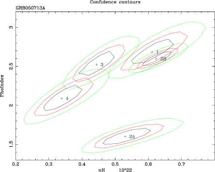
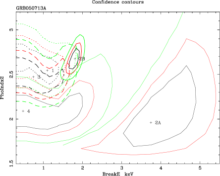
Figure 6: a) Left panel: single power law $\Gamma-N_{\rm H}$ $\chi^{2}$ confidence contours for the five WT spectra; b) right panel: broken power law $\Gamma_{2}-E_{\rm break}$ $\chi^{2}$ confidence contours for the five WT spectra.

5 Late-time “energy injection”?

Rebrightenings and bumps in the afterglow light curve are generally due to either density inhomogeneities in the interstellar medium or to “energy injections” at later times. The latter could be produced by slower shells that catch up with the afterglow shock at later times. We will consider both possibilities and show that the energy injection model is favored by the data. Another possibility is that such flares are produced by late internal shocks, i.e. slower shells colliding with each other before deceleration (e.g. Fan & Wei 2005; Zhang et al. 2005).

First, let us consider the single powerlaw fit to the spectral data. During the time decay phases (time intervals WT1 and WT2b in Figure 5), the single power law spectrum (Table 2) is consistent with $F_{\nu}\propto\nu^{-1.6}$. On the other hand, during the rise phase WT2a, $F_{\nu}\propto\nu^{-0.5}$ as in the standard synchrotron model (e.g. Sari, Narayan & Piran 1998). In this model, the changes of spectral slopes suggest that during the rise time the synchrotron frequency $\nu_{m}$ sweeps across the observation band (0.5–10 keV). This is impossible to achieve with a density bump, since $\nu_{m}$ is independent of the density for a completely adiabatic evolution, and almost independent of the density $n$ ($\nu_{m}\propto n^{-1/14}$) in a fully radiative evolution. Therefore, we consider the possibility that the rebrightenings are the result of energy injections.

A simple argument then shows that the synchrotron frequency is likely to vary within the 0.5–10 keV band covered by the XRT observation, and not be outside of the band as implied by the single powerlaw fit to the data. Indeed, for a completely adiabatic evolution, one has $\nu_{m}\propto E^{0.5}$ (where E is the burst energy), while for a fully radiative evolution $\nu_{m}\propto E^{4/7}$, both implying that the flux rebrightening $F_{2}/F_{1}$ scales with the frequency change factor as $\left(\nu_{m,2}/\nu_{m,1}\right)^{2}$. If the synchrotron frequency were outside the observation band (i.e. at an energy ${{}_{<}\atop{}^{\sim}}0.5$ keV before the beginning of the rebrightening, and ${{}_{>}\atop{}^{\sim}}10$ keV after the end of the rebrigthening), then it would need to vary by a factor ${{}_{>}\atop{}^{\sim}}20$, implying an energy injection $\left(\nu_{m,2}/\nu_{m,1}\right)^{2}\geq 400$. The rebrightening implied by this model is much larger than that seen in the data, $F_{2}/F_{1}\sim 10$, implying that the synchrotron frequency lies within the 0.5–10 keV band. For this reason we consider more physical the broken power law fits in Table 3. The most striking feature from these fits is that the break frequency is smaller than 1.6 keV in the WT1 spectrum and increases up to several keV in the WT2a spectrum (flux rebrightening) and then decreases again at energies $<$ of 1-2 keV at later times. This is consistent with the flat optical to X-ray spectral index from Figure 1 at 150-190 seconds after the trigger, indicating that, if the fast cooling regime applies, at this time the synchrotron frequency is between the X-ray and the optical band.

For the same reasons discussed above, the shift of the synchrotron frequency could not have been caused by a density bump. On the other hand, in the energy injection scenario, a flux rebrightening by a factor of 10 would have been produced by an increase in break frequency by a factor of about 3, fully consistent with the data.

Let us consider now the temporal behavior of the rebrightening as a function of the energy (sections WT2a and WT2b of the light curve in figure 5). Our analysis shows that the temporal power law index $\alpha_{r}$ during the rise time (section WT2a) is consistent with the constant value $\alpha_{r}=0.6$ in all the spectral bands. During this phase, the temporal evolution is indeed dominated by the time-dependent energy supply, which is independent of the frequency band. The temporal flux decay index $\alpha_{d}$ during the decay phase WT2b is shown in Figure 3. The lowest and highest energy bands are consistent with straddling the synchrotron frequency $\nu_{m}$ for an index $p=2$ of the power-law distribution of electrons, further confirming the broken power-law interpretation. Let us clarify this point. In the low energy band ($<2$ kev), the flux can be written as $F_{\nu}\propto(\nu/\nu_{c})^{-1/2}F_{\nu,\rm max}\propto t^{\alpha_{1}}$, while in the high energy band $F_{\nu}\propto(\nu_{m}/\nu_{c})^{-1/2}(\nu/\nu_{m})^{-p/2}F_{\nu,max}\propto t^{\alpha_{2}}$ where $\alpha_{1}$ and $\alpha_{2}$ are the power law indices of the decay in the low and high energy band respectively (Sari, Piran & Narayan 1998). We get a good fit to the data with $\alpha_{1}=-0.25$ and $\alpha_{2}=-3p/4+1/2$. The dashed line in figure 3 shows the results of this model for two values of $p$, $p=2$ and $p=2.5$.

Taken at face value, the value of p which fits best the decay indices in figure 3 is somewhat different from the value implied by the $\Gamma$ which fits best the spectrum during the decay phase WT2b, $p\sim 3$. However it should be considered that our description of the data is clearly over-simplified, and that statistical and systematic uncertainties in our determination of $\alpha_{d}$ and $\Gamma$ can certainly alleviate this discrepancy. In conclusion, we find remarkable that, at least qualitatively, the energy injection model in the framework of the afterglow theory is able to reproduce both the spectral and the temporal behavior observed in GRB 050713A.

The time lags between the light curves in the six energy bands considered here can be further used to constrain the product of the magnetic field energy fraction $\epsilon_{B}$, the burst energy, $E$, and the density of the external medium, $n$, $\epsilon_{B}^{-3}E_{52}^{-1}n_{1}^{-2}$, using the expression of the synchrotron cooling time given by Sari, Piran & Narayan (1998). The two curves in Figure 4 show the expected time lags for $\epsilon_{B}^{-3}E_{52}^{-1}n_{1}^{-2}=10^{-5}$ and $2\times 10^{-5}$. It is interesting to note that the synchrotron model does predict a time lag of the order of 6–9 s between the low energy photons ($<1$ keV) and higher energy photons (2–10 keV), and a flattening of the time lag for energies $>2$ keV as observed.

6 Summary

We have presented time and spectral analysis of GRB 050713A, whose light curve displays several rebrigthenings both in the $\gamma$-ray and in the X-ray bands. Our time-resolved spectral analysis has allowed us to conclude that the rebrigthenings are most likely due to late energy “injections”. Since the main energy output of the GRB engine rapidly decays with time (Janiuk et al. 2004), the energy injections are likely due to either slower shells generated during the prompt phase of the GRB engine and catching up at later times, or to later energy production by, for example, disk fragments that accrete at later times (Perna et al. 2006).

We would like to emphasize two conclusions that came out from the analysis of the light curve of GRB050713A. First the behavior of the time lags between the light curves in the six energy bands is consistent with what expected from synchrotron cooling. Second, the spectral index of the first decay spectrum WT1 is consistent with that of the decay from the main flare WT2b, thus suggesting that the WT1 is actually the tail of a flare coincident with the flare detected by BAT.

The X-ray light curve may present features detected in many Swift bursts (Chincarini et al. 2005, Nousek et al. 2005, Burrows et al. 2005b). In particular we notice that the XRT decay index starting 200 s after the trigger is flatter than the decay index during the XMM observation at about 8 hours from the trigger. This implies that a break should occur between 5000 s and 20.000 s after the trigger. The decay index after the break appears consistent with the predictions of the uniform ISM afterglow model, while the decay index before the break is much shallower. This shallow-to-normal decay may be due to the cessation of the refreshed shock phase. However we cannot exclude that this is a jet break due to the deceleration of the outflow. The break occurs at a time when the bulk Lorentz factor of the shock has slowed to $\Gamma\sim 1/\theta_{jet}$ (Rhoads 1997).

All optical points seem to be typical of the afterglow emission produced by an external forward shock. The optical flux varies with time as $F_{\nu}\sim t^{-0.67}$, which is consistent with the afterglow decay during the radiative evolution, $F_{\nu}\sim t^{-4/7}$. We should notice that this temporal behavior is similar to the X-ray one between WT4 and XRT-PC.

This research has been partially supported by ASI grant I/R/039/04 and MIUR. RP acknowledges support from NASA under grant NNG05GH55G, and from the NSF under grant AST 0507571. We warmly thank the Telescopio Nazionale Galileo and Liverpool Telescope teams for precious help in data acquisition. CG and AG acknowledge their Marie Curie Fellowships from the European Commission. CGM acknowledges financial support from the Royal Society. AM acknowledges financial support from PPARC. The Liverpool Telescope is operated on the island of La Palma by Liverpool John Moores University at the Observatorio del Roque de los Muchachos of the Instituto de Astrofisica de Canarias

References

- (1) Bersier, D. et al. 2002, ApJ, 584, L43
- (2) Bertin, E., & Arnouts, S. 1996, A&AS, 117, 393
- (3) Bjornsson, G., et al., 2004, ApJ 615, L77
- (4) Burrows, D. N., et al., 2005, Science 309, 1833B
- (5) Burrows, D. N., et al., 2005b, astro-ph/0511039, ”X-Ray Universe 2005 conference proceedings”.
- (6) Capalbi, M., Perri, M., Saija, B., Tamburelli, F., Angelini, L, 2005, “The SWIFT XRT Data Reduction Guide” http://heasarc.gsfc.nasa.gov/docs/swift/analysis/xrt_swguide_v1_2.pdf
- (7) Chincarini, G., Mangano, V., Moretti, A., et al. 2005, astro-ph/0511107, ”X-Ray Universe 2005 conference proceedings”.
- (8) De Ugarte Postigo, A. et al., 2005, A&A 443, 841.
- (9) De Luca, A. et al. 2005, GCN3695
- (10) Dickey, J. M. & Lockman F. J., 1990 ARA& 28,215.
- (11) Falcone, A., et al, 2005, GCN3581
- (12) Falcone, A.D., Burrows, D.N., Romano, P., et al. 2006, ApJ in press, astrp-ph/0511107
- (13) Fan, Y.Z., & Wei, D.M. 2005, MNRAS, 364, L42
- (14) Gao, W. H., 2005, astro-ph/0512646
- (15) Gehrels et al, 2005, ApJ 621, 558.
- (16) Golenetskii, S., et al., 2005, GCN 3619.
- (17) Granot, J., Nakar, E. & Piran, T., 2003, Nature 426, 138
- (18) Guidorzi, C. et al., 2006, PASP, in press, astro-ph/0511032
- (19) Guziy, S., Castro-Tirado, A.J., de Ugarte Postigo, A., Gorosabel, J., de León Cruz, J., Bogdanov, O., & Jelínek, M. 2005, GCN Circ. 3584
- (20) Hearty, F., Stringfellow, G., Lamb, D.Q., et al. 2005, GCN Circ. 3583
- (21) Heyl, J.S. & Perna, R. 2003, ApJ, 586, L13
- (22) Huang, Y. F., Cheng, K.S. & Gao, T.T. 2006, ApJ 637, 873.
- (23) King, A., O’Brien, P. T., Goad, M. R., Osborne, J., Olsson, E., & Page, K. 2005, ApJ, 630, L113
- (24) Janiuk, A., Perna, R., Di Matteo, T. & Czerny, B. 2004, MNRAS, 355, 950
- Jansen et al. (2001) Jansen, F., Lumb, D., Altieri, B., et al. 2001, A&A, 365, L1
- (26) Laursen, L.T., & Stanek, K.Z. 2003, ApJ, 597, L107
- (27) Lazzati, D., et al. 2002, A&A, 396, L5
- (28) Loiseau N. et al. 2005, GCN#3594
- (29) Malesani D., D’Avanzo, P., Palazzi, E., Israel, G.L., Chincarini, G., Stella, L., & Pedani, M. 2005, GCN Circ. 358
- (30) MacFadyen, A. I., Ramirez-Ruiz, E., & Zhang, W. 2005, astro-ph/0510192
- (31) Matheson, T. et al. 2002, ApJ, 582, L5
- (32) Monfardini, A., Gomboc, A., Guidorzi, C., et al. 2005, GCN Circ. 2588
- (33) Nakar, E., Piran, T., & Granot, J. 2003, New Astronomy, 8, 495
- (34) Nousek, J. A. et al. 2005, ApJ submitted, astro-ph/0508332
- (35) O’Brien, P. T. et al. 2006, ApJ, submitted, astro-ph/0601125
- (36) Perna, R., Armitage, P. J. & Zhang, 2006, ApJ, 636L, 29
- (37) Proga, D. & Zhang, B. 2006, astro-ph/0601272
- (38) Romano, P., Moretti, A., Banat, P.L., et al. 200, A&A, in press, astro-ph/0601173
- (39) Rhoads, J. E. 1997, ApJ, 487, L1
- (40) Sari, R., Piran, T, & Narayan, R., 1998, ApJ 497, L17
- (41) Sari, R. & Piran, T, 1999, ApJ 520, 641
- (42) Smith et al., 2002, Astron.J. 123, 2121
- Strűder et al. (2001) Strüder, L., Briel, U., Dennerl, K., et al. 2001, A&A, 365, L18
- (44) Tagliaferri, G. et al. 2005, Nature 436, 985
- Turner et al. (2001) Turner, M.J.L., Abbey, A., Arnaud, M., et al. 2001, A&A, 365, L27
- (46) Wren, J., Vestrand, W.T., Wozniak, P., White, R., & Evans, S. 2005, GCN Circ. 3604
- (47) Zhang, B., et al. 2005, ApJ, in press, astro-ph/0508321