Bolocam Survey for 1.1 mm Dust Continuum Emission in the c2d Legacy Clouds. II. Ophiuchus

Abstract

We present a large-scale millimeter continuum map of the Ophiuchus molecular cloud. Nearly 11 square degrees, including all of the area in the cloud with $A_{V}\geq 3$ magnitudes, was mapped at 1.1 mm with Bolocam on the Caltech Submillimeter Observatory (CSO). By design, the map also covers the region mapped in the infrared with the Spitzer Space Telescope. We detect 44 definite sources, and a few likely sources are also seen along a filament in the eastern streamer. The map indicates that dense cores in Ophiuchus are very clustered and often found in filaments within the cloud. Most sources are round, as measured at the half power point, but elongated when measured at lower contour levels, suggesting spherical sources lying within filaments. The masses, for an assumed dust temperature of 10 K, range from 0.24 to 3.9 M_⊙, with a mean value of 0.96 M_⊙. The total mass in distinct cores is 42 M_⊙, 0.5 to 2% of the total cloud mass, and the total mass above 4 $\sigma$ is about 80 M_⊙. The mean densities in the cores are quite high, with an average of $1.6\mbox{${}\times 10^{6}$}$ cm^-3, suggesting short free-fall times. The core mass distribution can be fitted with a power law with slope $\alpha=2.1\pm 0.3$ for $M>0.5$ M_⊙, similar to that found in other regions, but slightly shallower than that of some determinations of the local IMF. In agreement with previous studies, our survey shows that dense cores account for a very small fraction of the cloud volume and total mass. They are nearly all confined to regions with $\mbox{$A_{V}$}\geq 9$ mag, a lower threshold than found previously.

1 Introduction

For over 30 years, astronomers have known that stars are born in molecular clouds. However, the fraction of cloud mass that forms stars is usually small (Leisawitz et al., 1989), and the crucial step seems to be the formation of dense cores, which are well traced by dust continuum emission. Understanding the processes that control the formation of dense cores within the molecular cloud is necessary for understanding the efficiency and distribution of star formation (Evans, 1999). Progress in this area requires complete maps of large molecular clouds in the millimeter continuum emission, which traces the location, mass, and other properties of the dense cores. Such maps are becoming feasible only with the arrival of millimeter-wave cameras such as Bolocam.

One well-known birthplace of stars is the Ophiuchus molecular cloud. Located at a distance of $125\pm 25$ pc (de Geus, de Zeeuw, & Lub 1989), Ophiuchus contains the L1688 dark cloud region, which contains the Ophiuchus cluster (16^h 27^m, $-$24^∘ 30′ (J2000)) of young stars and embedded objects. The cluster region has been studied in great detail at a variety of wavelengths from millimeter molecular lines (Loren 1989; Ridge et al. 2006) to near-infrared (e.g., Wilking et al. 1989; Allen et al. 2002) to X-ray (Imanishi et al., 2001). It has also been mapped in dust continuum emission (Johnstone et al. 2000; Motte, André, & Neri 1998). The embedded cluster is itself surrounded by a somewhat older population of stars extending over 1.3 deg² (Wilking et al., 2005). The cloud is home to two other known regions of star formation, the Lynds dark clouds L1689 (16^h 32^m, $-$24^∘ 29′) and L1709 (16^h 31^m, $-$24^∘ 03′). However, little is known about star formation outside of these three regions.

In this paper, we present the first large-scale millimeter continuum map of the entire Ophiuchus molecular cloud. Maps at millimeter wavelengths of the dust continuum emission find regions of dense gas and dust, both those with embedded protostars and those that are starless. Previously published maps of the Ophiuchus cloud covered only small regions: Motte, André, & Neri (1998) mapped about 0.13 deg² at 1.3 mm and Johnstone et al. (2000) mapped about 0.19 deg² at 850 µm. A larger (4 deg²) map at 850 µm is referred to but not published by Johnstone, Di Francesco, & Kirk (2004); it will be shown in Ridge et al. (2006). Most recently, Stanke et al. (2005) have mapped a 1.3 deg² area of L1688 at 1.2 mm. Our map covers 10.8 deg², providing a total picture of the dense gas in Ophiuchus.

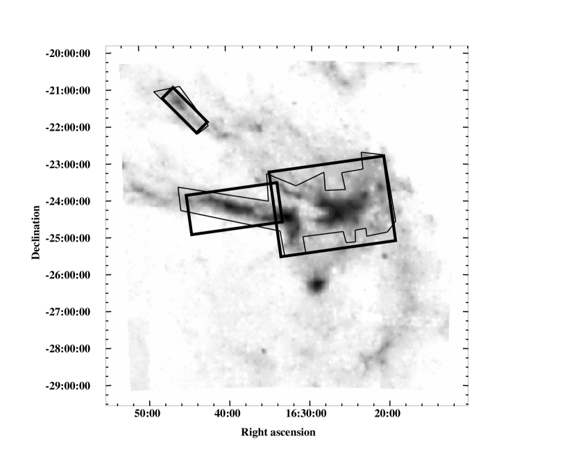
Figure 1: Extinction map of Ophiuchus from Cambrésy (1999) with the outline of the Bolocam observation area (thick lines) and the Spitzer IRAC observation area (thin lines). The area observed with IRAC was chosen to cover the cloud down to $A_{V}\geq 3$. The Bolocam observations were designed to cover approximately the same region observed with IRAC.

Our survey complements the Spitzer c2d Legacy project “From Molecular Cores to Planet-forming Disks” (Evans et al., 2003). All of the area in the cloud with $A_{V}\geq 3$ magnitudes (according to the map of Cambrésy (1999)) was observed with Bolocam and the InfraRed Array Camera (IRAC) on Spitzer (Figure 1). A somewhat larger area was also mapped at 24, 70, and 160 µm with the Multiband Imaging Photometer for Spitzer (MIPS). Maps of millimeter molecular line emission for this same area have been made by the COMPLETE team (Goodman 2004; Ridge et al. 2006). Previously, the largest maps of molecular lines were those of Loren (1989) and Tachihara, Mizuno, & Fukui (2000).

In addition to Ophiuchus, two other clouds were mapped with both Bolocam and Spitzer by the c2d team, Perseus (Enoch et al. 2006, hereafter Paper I) and Serpens (Enoch et al. 2006, in prep.). This paper is the second in a series describing these observations and applies the analysis methods described in Paper I. The results for Ophiuchus will be compared to those for Perseus in §4.3.

2 Observations

We mapped the Ophiuchus molecular cloud at 1.12 mm (hereafter 1.1 mm for brevity) with Bolocam on the CSO during two observing runs: 21 May – 09 June 2003 and 06 – 11 May 2004. Bolocam is a 144-element bolometer array camera that operates at millimeter wavelengths (Glenn et al., 2003). In May 2003, there were 95 channels; in May 2004, the observations were taken with 114 channels. The Bolocam field of view is $7\farcm 5$, the beams are well described by a Gaussian with a FWHM of 31″ at 1.1 mm, and the instrument has a bandwidth of 45 GHz. The cloud was observed in three main sections: the main part, including the L1688 cluster region, the large eastern streamer that extends to the east of L1689, and a smaller northeastern streamer. The map of the northeastern streamer is not contiguous with the other regions, as shown in Figure 1.

Each section was observed by scanning Bolocam at a rate of 60″ per second without chopping. Each subsequent subscan was offset from the previous one by 162″ perpendicular to the scan direction. With this scan pattern, 1 square degree was observed with 23 subscans in approximately half an hour of telescope time, including 20-second turn-around times at the edges of the maps.

Each section of the map was scanned in two orthogonal directions, rotated slightly from right ascension (RA) and declination (Dec) by small angles. This technique allows for good cross-linking of the final map with sub-Nyquist sampling and minimal striping from $1/f$ noise. The northeastern streamer is a little more than 0.5 deg², the eastern streamer section is about 2.7 deg², and the large L1688/main cloud section covers a total of 7.4 deg², which was observed in four sections of approximately 4 deg² each.

The best-weather observations from both runs for each of the three sections were averaged and combined into a single large map: six observations of the northeastern streamer were averaged, three in RA and three in Dec, for a total observation time of about 4.4 hours. The eastern streamer sections consists of five observations (three RA and two Dec scans) for a total observation time of 6 hours. The main cloud region was observed in four pieces, each observed four times (two RA and two Dec scans), which required thirteen hours of integration time. The resulting coverage varies by $\sim 25$%.

In addition to the maps of Ophiuchus, small maps of secondary calibrators and pointing sources were made every 2 hours throughout the run. All calibration sources observed throughout each run were used to derive the flux calibration factor for that run. Planets provided beam maps and primary flux calibration sources. Uranus and Mars were observed during both runs. Neptune was also observed on the May 2004 run.

3 Data Reduction

3.1 Pointing and Flux Calibration

Beam maps were made from observations of Uranus, Mars, and Neptune, and a pointing model was generated with observations of these planets, Galactic HII regions, and the protostellar source IRAS 16293$-$2422, which lies in the Ophiuchus cloud complex. For May 2004, the root-mean-square (rms) pointing uncertainty derived from the deviations of IRAS 16293$-$2422 centroids from the Bolocam/CSO pointing model is 2 to 3″; however, the number of IRAS 16293$-$2422 observations is small (seven), so the rms is not well-characterized. For May 2003, the rms pointing uncertainty was 6″, based on the dispersion of the centroid of IRAS 16293$-$2422 after the pointing model was applied.

A flux density calibration curve was generated for each run from observations of Uranus, Neptune, and secondary calibrators (Sandell 1994) throughout each night and over a range of elevations, thereby sampling a large range in atmospheric optical depths. With Bolocam, an AC biasing and demodulation technique is used to read out the bolometers. Fluctuations in the carrier amplitude correspond to changes in the bolometer resistance in response to changes in optical power. On long timescales ($>1$ scan), variations in atmospheric opacity, or loading, cause changes in flux density calibration from both the signal attenuation and the change in the bolometers’ responsivities induced by the loading changes. Thus, the bolometer resistances can be used to track calibration on a scan-by-scan basis. The flux densities were calibrated from the loading for each observation using the composite calibration curve built up from the entire run. This method is superior to photometric calibration procedures that require interpolation in time or extrapolation across large ranges in elevation.

3.2 Iterative Mapping and Sensitivity to Extended Sources

The data were reduced using an IDL-based reduction package written for Bolocam (http://www.cso.caltech.edu/bolocam/). The basic pipeline was described in Laurent et al. (2005) and procedures unique to observations of molecular clouds (large area maps with high dynamic ranges and extended structures) were described in Paper I. Here we summarize the techniques and refer the reader to those papers for details and results of simulations that characterized the algorithms.

With Bolocam’s AC bolometer bias and lock-in scheme, observations are made by scanning the telescope without chopping the CSO subreflector. The AC bias and rapid scanning modulate the signals above the atmospheric $1/f$ knee; residual atmospheric emission (“background”) is removed by sky subtraction, or “cleaning”. Bolocam was designed so that the bolometer beams overlap in the telescope near field, resulting in predominantly common-mode atmospheric background. This background was subtracted using a principle component analysis (PCA) that removed signals that were common mode across the focal plane array from the raw bolometer voltage time streams. While sky background is effectively removed in this manner, source flux densities are attenuated too, especially in the case of extended sources which have significant common-mode components. The first common-mode component is essentially the mean of all the bolometer signals. Removal of successive orthogonal components subtracts more sky background, but each component also subtracts more from the source flux densities. Experimentation showed that removal of three PCA components removed the majority of the striping and sky background, 20% to 30% more than a simple mean subtraction.

Cleaning with bright sources in the field results in negative sidelobes along the scan direction because the mean timestreams, obtained by averaging over all bolometers, are set to zero by subtraction of the first common-mode component. Thus, the sources sit in negative bowls and the total flux densities for large (120″) bright sources can be attenuated by as much as 50%. This problem is remedied with an iterative mapping procedure in which sky subtraction is successively improved by removing a source model from the raw data and re-cleaning to recover structure missing from the original map (see Paper I).

Simulations with fake sources of various sizes and signal-to-noise ratios showed that five or fewer iterations yield a nearly complete recovery of flux densities for bright point sources ($\sim 98$% recovery). Flux densities of large, faint sources with widths several times the beam size and amplitudes at approximately the level of the map rms noise are not recovered as well, with as much as 10% of the flux density missing after 20 iterations. However, we restrict our photometry to small apertures and enforce a 4-$\sigma$ detection threshold, so the impact on our catalog is small. We adopt a conservative 5% photometric uncertainty from sky subtraction after iterative mapping. All source flux densities will be biased low, but by less than this amount.

The iterative mapping procedure was run for each section of Ophiuchus and for each observing run. The May/June 2003 data and May 2004 were iteratively mapped separately because they required different calibration and pointing corrections. The final map is a weighted average of the maps from each run.

3.3 Source Identification

After the final calibrated maps were created, sources were identified as in Paper I. First, the maps were optimally filtered for point source detection, using a filter accounting for the beam size, telescope scan rate, and system noise Power Spectral Densities (PSDs), hereafter a Wiener filter, as described in Paper I. The Wiener filtering attenuates the 1/$f$ noise and reduces the rms per pixel by about $\sqrt{3}$. Then, the map was trimmed to cut off the edges where the coverage was low. The coverage is dependent upon the number of observations, the number of bolometers that were read out, and the scan strategy. The average coverage in the map varies from 40 hits per pixel (a hit means that a detector passed over this area on the sky), corresponding to 20 s of integration time, in most of the L1688 region to 60 (30 s of integration time) in the northeastern streamer. If the coverage was less than 0.22 times the maximum coverage (corresponding to a range in the local rms over the map of a factor of $\sim 2$) then that part of map was not included in the analysis. Finally, a source-finding routine found all the peaks in the Wiener-filtered map above 4 $\sigma$ in the rms map.

A detection limit as low as 4 $\sigma$ was necessary to detect some previously known sources, but this limit was not low enough to eliminate all false detections identified by the source extraction procedure. Some artifacts were incorrectly identified as sources. Therefore, each source was inspected by eye. Most of the artifacts were unambiguous because they were found close to the edges of the map or were caused by striping: one pixel wide and extended in one of the scan directions. Single-pixel peaks were also discarded, which might have resulted in excluding some faint sources. Although in principle it should be possible to recover structure up to the array size of $7\farcm 5$, it was found in Paper I that structures $\gtrsim 4\arcmin$ are severely affected by cleaning, and not well recovered by iterative mapping.

4 Results

4.1 General cloud morphology

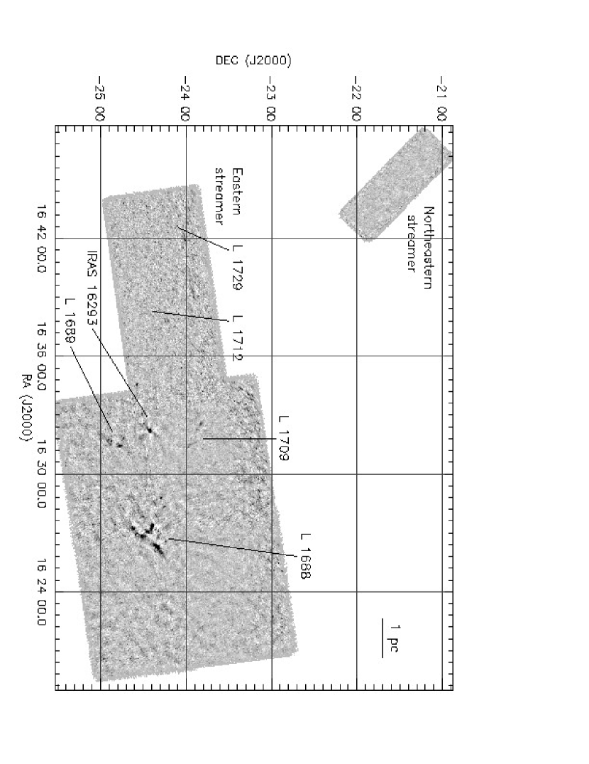
Figure 2: 1.1 mm Bolocam map of 10.8 deg² (51.4 pc² at $d=125$ pc) in the Ophiuchus molecular cloud, with $10\arcsec$ pixels and a beam size of $31\arcsec$. The gray scale is proportional to intensity weighted by the coverage to avoid confusion by noise in regions with low coverage. Well known regions and those discussed by name in the text are indicated.

The map of the cloud is shown in Figure 2, with known regions identified. Our map covers 10.8 deg² (51.4 pc² at a distance of 125 pc), which is equivalent to $1.4\times 10^{5}$ resolution elements given the beam size of $31\arcsec$. Most of the compact emission is confined to the L1688 cluster region. Several sources are also detected in L1709, L1689, and around the extensively studied Class 0 protostar IRAS 16293$-$2422. No emission that is extended $\gtrsim 2\arcmin$ is seen in the map.

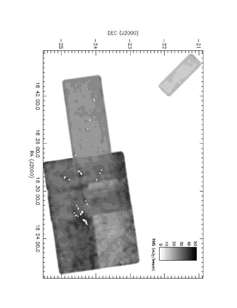
Figure 3: A map of the noise in gray scale with sources indicated by white plus signs. The gray scale runs from 11 mJy beam^-1 to 30 mJy beam^-1. High noise regions are apparent in a strip above L1709, and in the area containing L1688. Note the increased noise near bright sources caused by residual systematics from sky subtraction.

The noise in the final map varied from section to section because of differences in the number of good observations and changes in sky noise. A map of the noise (Fig. 3) shows the variations in noise in the different map areas, ranging from 11 to 30 mJy beam^-1. The average rms in the regions of the map where most sources were detected was about 27 mJy beam^-1. High noise regions are apparent in Figure 3 as a strip above L1709 and in the regions around strong sources, especially in the L1688 cluster.

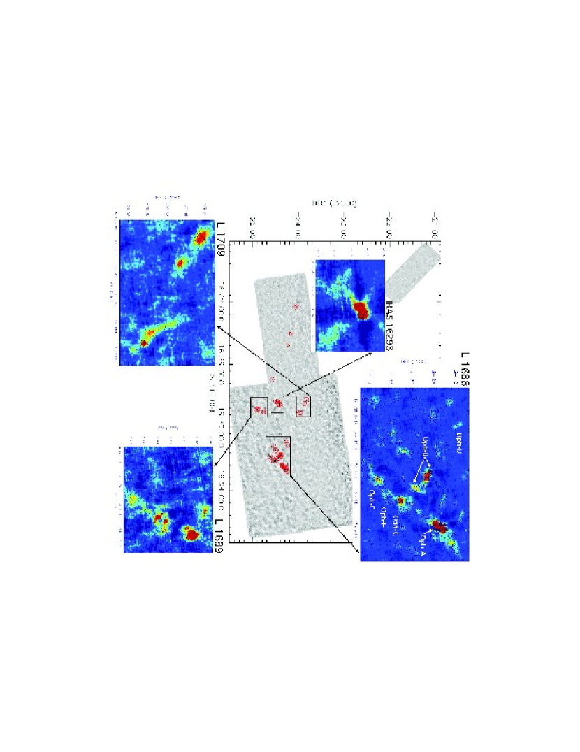
Figure 4: 1.1 mm Bolocam map of the Ophiuchus molecular cloud, with the positions of the 44 sources detected above 4 $\sigma$ marked as circles. The gray scale shows the intensity not weighted by the coverage. The inset maps show particular regions on an expanded scale. The conversion from intensity to color differs among the insets to cover the large range of intensity. Sources marked by triangles in the eastern streamer are below the 4-$\sigma$ detection limit so are tentative detections (but see Fig. 5).

We detected 44 sources with signal-to-noise greater than 4 $\sigma$ that were confirmed as real by inspection. These are listed in Table 1 and identified for convenience as Bolo 1, etc. All of these sources were identified in the main cloud and eastern streamer sections. Figure 4 plots the positions of the sources as red circles on the grayscale 1.1 mm map, with insets showing magnifications of the densest source regions. We did not detect any sources in the northeastern streamer, where the noise is lowest. Most of the sources are concentrated in the previously well-studied regions in Ophiuchus, suggesting that dense cores are highly clustered in the Ophiuchus cloud. Figure 4 contains blow-ups of the main regions of emission, including the well known Ophiuchus cluster in L1688, L1689, IRAS 16293$-$2422, and L1709.

Visual comparison to previous maps of dust continuum emission in the L1688 cluster indicates reasonable agreement on the overall shape of the emission, considering differences in resolution (Motte, André, & Neri, 1998) and wavelength (Johnstone et al., 2000). However, detailed comparison of source positions in Table 1 and those in Johnstone et al. (2000) shows that a substantial number of our sources are separated into multiple sources by Johnstone et al. (2000), who used the the clumpfind algorithm on data with better resolution by a factor of two; in the same area, they list 48 sources compared to our 23. The list of 48 includes some small, weak, but unconfused sources that we do not see. Assuming that $S_{\nu}\propto\nu^{3}$, as expected for emission in the Rayleigh-Jeans limit with an opacity proportional to $\nu$, some of these sources should still lie above our detection limit, but not far above.

The Stanke et al. (2005) map covers 1.3 deg² of L1688 (slightly less than one of the boxes defined by the grid lines in Fig. 2), with lower noise ($\sim 10$ mJy) and a slightly smaller beam (24″) at nearly the same wavelength (1.2 mm). Their images are qualitatively very similar to the L1688 inset image in Fig. 4. However, they find 143 sources in this region, using wavelet analysis and clumpfind, and by essentially cleaning down to the noise. They include sources that are less than 3 $\sigma$ but extended. These differences make it difficult to compare sources in detail, but it appears that many of our sources would be split into multiple sources by Stanke et al. (2005).

Another useful comparison is with the work of Visser et al. (2002) in a less crowded area of Ophiuchus. They found 5 sources along a filament in L1709; we find three sources in reasonable agreement in position, while L1709-SMM3 and L1709-SMM5 from their paper are blended into Bolo 30 in Table 1. We see additional structure below the 4-$\sigma$ limit extending to the northeast of that group of sources that is not seen in the Visser et al. (2002) map. The most diffuse source in their map, L1709-SMM4, shows up strongly in our map, but shifted about 25″ east, an example of position shifts caused by different sensitivity to large scale structure and source finding algorithms. Visser et al. (2002) also found a weak source in L1704 that we do not see, consistent with our detection limit. These points should be borne in mind when we compare source statistics to those of previous work in later sections.

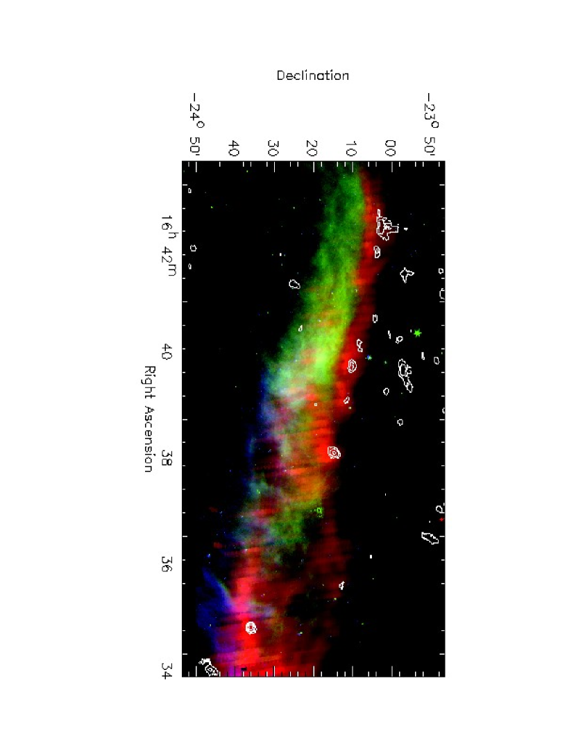
Figure 5: Emission at 1.1 mm seen with Bolocam in the eastern streamer (2, 3, 4, 6, 8 $\sigma$ contours) is overlaid on a three color image from Spitzer, with IRAC band 4 (8 µm) in blue, MIPS band 1 (24 µm) in green, and MIPS band 3 (160 µm) in red. The 160 µm map is incompletely sampled and saturated emission produces stripes. The 160 µm map has been smoothed, but artifacts remain. The 1.1 mm emission does line up with the relatively opaque part of the streamer, as indicated by weak emission at 8 µm and strong emission at 160 µm.

Several diffuse emission peaks were observed in the eastern streamer, an area that includes L1712 (16^h 38^m, $-$24^∘ 26′) and L1729 (16^h 43^m, $-$24^∘ 06′). However, these cores, though visible by eye in the map, are only 3-$\sigma$ detections and are listed separately as tentative detections in Table 1 and are not included in our source statistics. These sources are in a long filament of extinction that extends east from the main cloud (Cambrésy 1999; Ridge et al. 2006). We believe at least some of these sources are real, based on inspection by eye and comparison to Spitzer maps of the region. In Figure 5, the tentative 1.1 mm sources align with an elongated structure that is dark at 8 µm, but bright at 160 µm, suggestive of a cold, dense filament. This filament was previously observed in ¹³CO (Loren, 1989) and C¹⁸O (Tachihara, Mizuno, & Fukui, 2000), but it has not been mapped in the millimeter continuum until now. While the overall morphology is similar to that seen in C¹⁸O (Tachihara, Mizuno, & Fukui, 2000), only Bolo 45 has an obvious counterpart, $\rho$-Oph 10, in the table of Tachihara, Mizuno, & Fukui (2000).

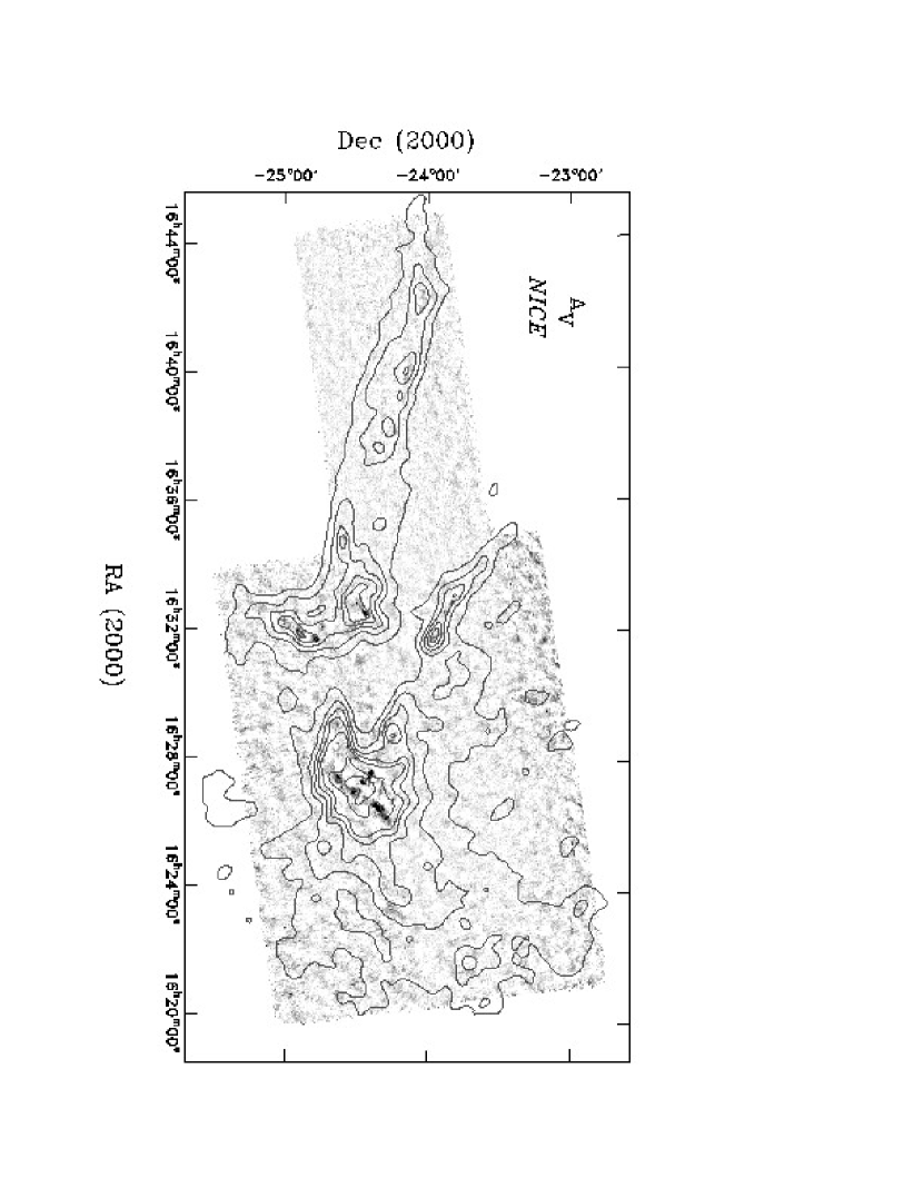
Figure 6: Visual extinction ($A_{V}$) contours calculated from 2MASS data using the ${\it{NICE}}$ method, overlaid on the grayscale 1.1 mm map. Contours are $A_{V}=2$, 4, 6, 8, 10, 15, and 20 mag with an effective resolution of $5\arcmin$.

The most striking feature of the Bolocam map of Ophiuchus is the lack of 1.1 mm emission in regions outside of known regions of star formation, even in areas with significant extinction ($A_{V}>$ 3 mag). Figure 6 shows the Bolocam map of Ophiuchus overlaid with extinction contours constructed using the NICE method (e.g., Lada et al. 1999; Huard et al. 2006), making use of 2MASS sources, and convolving the line-of-sight extinctions with a Gaussian beam with FWHM of 5′. This method depends on background stars to probe the column densities through the cloud. Similar to Enoch et al. (2006), we eliminate from the 2MASS catalog most foreground and embedded sources that would yield unreliable extinction estimates when constructing the extinction map. In order to calibrate the extinction map, we identified two “off-cloud” regions, which were free of structure and assumed to be non-extincted regions near the Ophiuchus cloud. These off-cloud regions contained a total of more than 13000 stars and were 0^∘6 $\times$ 0^∘6 and 1^∘5 $\times$ 0^∘2 fields centered on $\alpha$= 16^h44^m00^s, $\delta$= $-$22^∘54^′00^′′ and $\alpha$= 16^h39^m12^s, $\delta$=$-$25^∘24^′00^′′ (J2000.0), respectively. The mean intrinsic H$-$K color of the stars in these off-cloud fields was found to be 0.190 $\pm$ 0.003 magnitudes. We assume $\mbox{$A_{V}$}=15.9$ E(H–K) to convert to $A_{V}$ (Rieke & Lebofsky, 1985).

The 1.1 mm sources are all in regions of high extinction, but not all regions of substantial extinction have Bolocam sources. For example, we found no 1.1 mm sources in the small northeastern streamer of Ophiuchus that could be confirmed as real by eye despite having much lower noise in this region than for the rest of the map. The beam-averaged extinctions in the northeastern streamer are $A_{V}\approx 3$ to 8 magnitudes. The 4-$\sigma$ detection limit in this region corresponds to objects with masses as small as 0.06 M_⊙ (see §4.2). Thus even in relatively high extinction regions, much of the Ophiuchus cloud appears devoid of dense cores down to a very low mass limit.

4.2 Source Properties

4.2.1 Positions and Photometry

Table 1 lists the position, peak flux density, and signal-to-noise ratio (S/N) of the 44 4-$\sigma$ sources, and the four 3-$\sigma$ detections in the eastern streamer are listed separately. All statistical analysis is based on the 44 secure detections only. For known sources the most common names from the literature are also given. Some are known to host protostars while others may be starless. The peak flux density is the peak pixel value in the $10\arcsec$ pixel^-1 unfiltered map (without the Wiener filter applied). The uncertainty in the peak flux density is the local (calculated within a 400″ box) rms beam^-1 and does not include an additional 15% systematic uncertainty from calibration uncertainties and residual errors after iterative mapping. The S/N is calculated from the peak in the Wiener-convolved map compared to the local rms because this is the S/N that determines detection.

Source photometry is presented in Table 2. Aperture photometry was calculated using the IDL routine APER. Flux densities for each source are given in Table 2 within set apertures of 40″, 80″, and 120″. If an aperture is larger than the distance to the nearest neighboring source, the flux is not given, to avoid contamination of fluxes by nearby sources. Table 2 also lists the total flux density, which is integrated over a 160″ aperture or the largest aperture up to 160″ that does not include flux by nearby sources (defined such that the aperture radius is less than half the distance to the nearest neighbor). The uncertainties for the flux densities are $\sigma_{ap}=\sigma_{beam}\sqrt{\frac{A_{ap}}{A_{beam}}}$, where $\sigma_{beam}$ is the local rms beam^-1, and $A_{ap}$ and $A_{beam}=\pi\mbox{$\theta_{mb}$}^{2}/(4\ln 2)$ are the aperture and beam areas. The uncertainties in Table 2 do not include an additional 15% systematic uncertainty in the flux densities that results from the absolute calibration uncertainty (10%) and systematic biases remaining after iterative mapping (5% for bright sources).

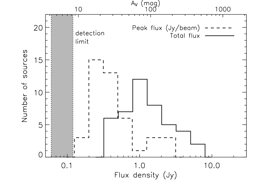
Figure 7: The distribution of the peak flux densities (dashed line) and total flux densities (solid line) of the 4-$\sigma$ sources. The peak flux density is the peak pixel value in the map, in Jy beam^-1. The top axis shows the value of $A_{V}$ inferred from the emission, using equation 2. The mean peak flux density of the sample is $0.6$ Jy/beam and the mean total flux is $1.6$ Jy. The 4-$\sigma$ detection limit varies from $0.06$ to $0.12$ Jy/beam across the map due to variations in the local noise, although most sources are detected in the higher noise regions. The range in noise in indicated by the shaded region.

The distribution of flux densities for the 44 detected sources is shown in Figure 7. This figure compares the distribution of peak flux densities to the total flux densities. The peak flux density distribution has a mean of $\sim 0.6$ Jy beam^-1. The total flux density distribution has a mean of about 1.6 Jy. The shaded region in Figure 7 indicates the 4-$\sigma$ detection limit, which varies throughout the map from $\sim 0.06-0.12$ Jy beam^-1. The flux density distributions shown in Figure 7 are similar to the distributions of peak and total flux densities of Bolocam sources in Perseus (Paper I) in that the total flux density distribution is shifted from the peak distribution because most sources are larger than the beam.

4.2.2 Sizes and Shapes

Sizes listed in Table 2 were found by fitting a 2D elliptical Gaussian to determine the FWHM of the major and minor axes and the position angle of the ellipse (PA), measured east of north. The errors are the formal fitting errors. There are additional uncertainties due to noise and residual cleaning effects on the order of 10 – 15% in the FWHM and $\sim 5$^∘ in the PA. The size of the source is limited by the distance to its nearest neighbor, because all emission at radii greater than half the distance to the nearest source is masked out for the Gaussian fit to avoid including flux from neighboring sources in the fit. This procedure also ensures that the size and the total flux density of a source are measured in approximately the same aperture. The sources in the L1688 cluster are quite crowded and source sizes and fluxes may be affected by nearby sources.

Figure 8 shows the distributions of the major and minor axis FWHMs from the fits. Both distributions peak between 50″ and 60″, and the average axis ratio is 1.2. Only a few sources have large FWHM sizes ($>100\arcsec$). Many of the sources in the map are part of filamentary structures. Individual sources are found by identifying peak pixels above a 4-$\sigma$ cutoff. Therefore, large clumps of emission are often broken down into several smaller sources, because the clumps contain several peaks. This method of finding cores and the filamentary nature of the dense gas in Ophiuchus could result in a slight elongation of the sources. However, the majority (61%) of sources in the entire sample are not elongated at the half maximum level (axis ratio $<$ 1.2), suggesting roughly spherical condensations along the filaments.

Morphology keywords for each source are also listed in Table 2, which indicate if the source is multiple (within 3′ of another source), extended (FW at 2 $\sigma>$ 1′), elongated (axis ratio at 4 $\sigma>$ 1.2), or weak (peak flux density is less than 8.7 times the rms beam^-1. Of the 44 sources, 18 are classified as round, with axis ratio at the 4-$\sigma$ level less than 1.2. The difference between this result and the fact that 61% had axis ratios from the Gaussian fits $<1.2$ indicates relatively round sources within more extended, elongated structures; this result suggests spherical sources embedded along filaments. Visual inspection indicates that the elongated lower contours are usually elongated along the local filametary structure, as seen both in the still lower contours and in the extinction map (Fig. 6). Future polarimetric observations could determine the role of magnetic fields in the filamentary structures. Of the 44 sources, 36 are multiple, reflecting the strongly clustered nature of the sources (see later section). Also 36 sources are extended. Only two sources are neither multiple nor extended. We see no evidence for a population of isolated, small, dense cores.

4.2.3 Masses, Densities, and Extinctions

Isothermal masses for the sources were calculated according to the equation

$$M=\frac{D^{2}S_{\nu}}{B_{\nu}(T_{D})\kappa_{\nu}}$$ (1)

where $D$ is the distance (125 pc), $S_{\nu}$ is the total flux density, $B_{\nu}$ is the Planck function, $T_{D}$ is the dust temperature, and $\kappa_{\nu}$ is the dust opacity. We interpolate from the dust model of Ossenkopf & Henning (1994) for grains with coagulated ice mantles (their Table 1, column 5), hereafter referred to as OH5 dust, to obtain $\kappa_{\nu}$ = 0.0114 cm² g^-1 at 1.12 mm. This dust opacity assumes a gas to dust mass ratio of 100, so the above equation yields the total mass of the molecular core. Table 2 lists the isothermal masses for a dust temperature of 10 K. The uncertainties in the masses listed in Table 2 are from the uncertainty in the total flux density. The total uncertainties include uncertainties in distance, opacity, and $T_{D}$, and are at least a factor of 4 (Shirley et al., 2002; Young et al., 2003, and see Paper I for a more complete discussion).

The total mass of the 4-$\sigma$ sources is 42 M_⊙, with $\mbox{$\langle M\rangle$}=0.96$ M_⊙, and a range from $0.24$ to $3.9$ M_⊙. The Johnstone, Di Francesco, & Kirk (2004) survey of Ophiuchus found a larger total mass (50 M_⊙) in a smaller area than we covered. Part of the difference results from their assumption of a larger distance (160 pc), which would make all their masses larger than ours by a factor of 1.6. However, they assume a value for $\kappa_{\nu}$ at 850 µm that is 1.1 times higher than OH5 dust, and they assume $\mbox{$T_{D}$}=15$ K, which would decrease our masses by a factor of 1.94. If we used the assumptions of Johnstone, Di Francesco, & Kirk (2004) for our data, we would derive a total mass of 32 M_⊙ from our data. The source of the difference between our result for total mass in cores and that of Johnstone, Di Francesco, & Kirk (2004) does not seem to be explained by the assumptions used to obtain mass. More likely, it arises from differences in methods of defining sources. If we integrate all the areas of the map above 4 $\sigma$, we get 131 Jy, which translates to 79 M_⊙, using our usual assumptions, or 60 M_⊙, using the assumptions of Johnstone, Di Francesco, & Kirk (2004). Thus about half the mass traced by emission cannot be assigned to a particular core, mostly because it is in confused regions. de Geus, de Zeeuw, & Lub (1989) estimate a total mass in Ophiuchus of $10^{4}$ M_⊙  while we find a total of 2300 M_⊙ above $\mbox{$A_{V}$}=2$ (Table 3). The percentage of cloud mass in dense cores is between 0.4% and 1.8%. This fraction is even lower than that found in in Paper I for Perseus (between 1% and 3%).

The mean particle density for each source is estimated as $\mbox{$\langle n\rangle$}=M/((4/3)\pi R^{3}\mu_{p}m_{H})$, where $M$ is the total mass, $R$ is the mean deconvolved HWHM size, and $\mu_{p}=2.37$ is the mean molecular weight per particle, including helium and heavier elements. The mean densities are quite high compared to the surrounding cloud, ranging from $\mbox{$\langle n\rangle$}=9\mbox{${}\times 10^{4}$}$ cm^-3 to 3${}\times 10^{7}$ cm^-3, with an average value of $1.6\mbox{${}\times 10^{6}$}$ cm^-3. The free-fall timescale for the mean density would be only $2.7\mbox{${}\times 10^{4}$}$ yr.

The beam-averaged column density of H₂ at the peak of the emission is calculated from the peak 1.1 mm flux density $S_{\nu}^{beam}$:

$$N(\mathrm{H}_{2})=\frac{S_{\nu}^{beam}}{\Omega_{beam}\mu_{H_{2}}m_{H}\kappa_{\nu}B_{\nu}(T_{D})}.$$ (2)

Here $\Omega_{beam}$ is the beam solid angle, and $\mu_{H_{2}}=2.8$ is the mean molecular weight per H₂ molecule, which is the relevant quantity for conversion to extinction. We assume a conversion from column density to $A_{V}$ of $N($H${}_{2})/A_{V}=0.94\times 10^{21}$ cm² mag^-1 (Bohlin et al., 1978), using $R_{V}=3.1$. This relation was determined in the diffuse interstellar medium and it may not be correct for such highly extinguished lines of sight as we are probing. Peak extinctions range from 11 to 214 mag for the 4-$\sigma$ sources with a mean value of 43, while the tentative detections in the eastern streamer range from 7 to 11.

The extinctions within the cores should be distinguished from the surrounding extinction, as traced by the NICE method with 2MASS sources. While 2MASS sources probe the low-to-moderate extinctions within the Ophiuchus cloud, the sensitivity of the 2MASS observations is not sufficient to probe reliably the high extinction regions traced by the millimeter emission. By considering both tracers of extinction, the morphology of the cloud can be inferred over a large range of column densities, from the diffuse and vast regions of the cloud (containing most of the mass) to the densest cores. Almost all the 1.1 mm emission lies within the contour of $A_{V}=10-15$ mag, as determined from the near-infrared (Fig. 6); the faint emission in the eastern streamer is the main exception. A quantitative comparison will be made in §5.4.

4.3 Comparison to Perseus (Paper I)

One considerable advantage to conducting a survey of several regions with the same instrument is the elimination of a number of biases that can result from observations with different instruments or at different wavelengths. Ophiuchus is the second cloud in a series of three large 1.1 mm surveys using Bolocam, including Perseus (Paper I) and Serpens (Enoch et al., in prep). Here we compare the results for Perseus and Ophiuchus.

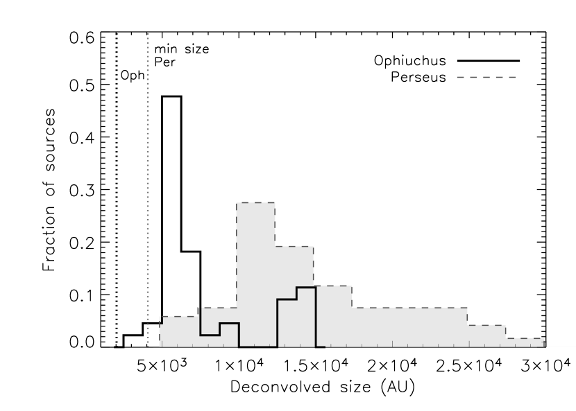
Figure 9: Comparison of the distribution of sizes of sources in Ophiuchus (heavy line) and Perseus (light line and gray-shaded). The fraction of total sources is plotted as a function of deconvolved source size in AU. The vertical dotted lines represent the size of the smallest resolvable source (heavy dotted for Ophiuchus and light dotted for Perseus).

The distribution of source sizes is considerably different for Ophiuchus and Perseus, especially if one considers the deconvolved source sizes, as illustrated in Figure 9, which plots the fractional number of total sources as a function of size. Perseus sources have a larger mean linear size than those in Ophiuchus ($1.5\times 10^{4}$ AU vs $7.6\times 10^{3}$ AU), and the Perseus distribution extends to $3\times 10^{4}$ AU, twice the maximum size of sources in Ophiuchus ($1.5\times 10^{4}$ AU). The fact that Ophiuchus is closer (125 versus 250 pc) could play a role, but the distributions in both clouds lie well above the resolution limits (vertical lines in Fig. 9). The largest recoverable size is about 240″, which corresponds to 3${}\times 10^{4}$ AU in Ophiuchus and 6${}\times 10^{4}$ AU in Perseus, larger than the relevant distributions in Fig. 9. However, in clustered regions, the size is limited by the nearest neighbors. The fraction of sources classified as multiple is somewhat higher (0.82) in Ophiuchus than in Perseus (0.73) and the ratio of mean separation to mean size is smaller in Ophiuchus than in Perseus (2.5 versus 3.0).

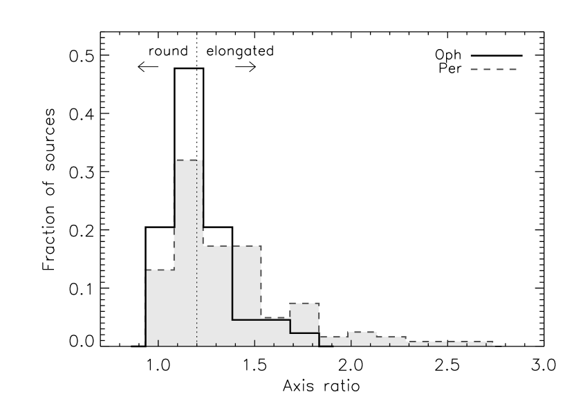
Figure 10: Comparison of the distribution of axis ratios (measured at the FWHM) of sources in Ophiuchus and Perseus (light line and gray-shaded). Sources with axis ratios $<1.2$ are considered round. There are a larger fraction of sources with axis ratios greater than 1.2 in Perseus than in Ophiuchus.

A comparison of the distribution of axis ratios for the two clouds (Figure 10) shows that sources in Perseus tend to be more elongated than those in Ophiuchus. In particular, the Perseus distribution has a tail that extends to much greater axis ratios. The mean axis ratio in Perseus is 1.4 compared to 1.2 in Oph. It was found in Paper I that axis ratios smaller than 1.2 are not significantly different from unity; thus sources in Ophiuchus are round on average, while sources in Perseus are elongated on average. The larger, more elongated sources in Perseus may be a real effect, or may be due, at least in part, to the different distances to the clouds. As noted above, many sources in Ophiuchus are round as measured by the axis ratio, but elongated as measured by the lower contours, possibly reflecting the effects of being in a filament. At greater distance, these small round cores may not stand out above the elongated lower level emission.

The mean mass of 0.96 M_⊙ is about half that in Perseus (2.3 M_⊙), but the smaller size of the sources in Ophiuchus makes the mean density higher ($\mbox{$\langle n\rangle$}=1.6\mbox{${}\times 10^{6}$}$ cm^-3 compared to $4.3\mbox{${}\times 10^{5}$}$ cm^-3 in Perseus) and the mean of the peak extinctions in the cores higher as well ($\mbox{$\langle A_{V}\rangle$}=43$ mag versus 25 mag for Perseus).

Further comparison to Perseus will be incorporated into various parts of §5.

5 Discussion

In the following sections, we discuss issues of completeness in the context of the mass-size relations, and then discuss the mass function of cores. We then discuss clustering tendencies and the extinction threshold.

5.1 Completeness

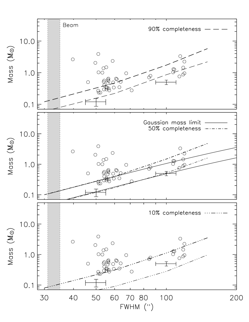
Figure 11: Distribution of source mass ($T_{D}$ = 10 K) versus FWHM size. The size is the geometric average of the FWHM of the major and minor axes as given in Table 1. The maximum size of the pointing-smeared beam is represented by the shaded regions. Solid lines are the 50% analytic mass detection limit as a function of size for Gaussian sources (Eq. 3). Empirical 90% (top panel), 50% (middle panel), and 10% (bottom panel) completeness limits are indicated, derived using Monte Carlo methods with simulated sources and taking into account the effects of cleaning, iterative mapping, and optimal filtering. Each completeness limit is calculated both in a low rms region (lower line) and a high rms region (upper line). Most real sources are found in the higher rms regions. Representative error bars for $50\arcsec$ and $100\arcsec$ FWHM sources near the detection limit are shown, as estimated from the results of Monte Carlo simulations.

Figure 11 shows the distribution of source mass versus size, where the size is the geometric average of the major and minor FWHM for each source. The minimum detectable mass and source size are related because we detect sources from their peak flux density, but calculate the mass from the total flux density. Therefore, we are biased against large, faint, low-mass sources. For Gaussian sources, the mass calculated from the total flux density is related simply to the mass from the peak flux density:

$$M_{limg}=M_{limp}(\theta_{s}/\theta_{b})^{2}\left[1-\exp(-4\ln 2(120/\theta_{s})^{2}\right],$$ (3)

where $M_{limg}$ is the mass limit for a Gaussian source, $M_{limp}$ is the mass limit for a point source, and $\theta_{s}$ and $\theta_{b}$ are the FWHM of source and beam, respectively. The last factor corrects for flux from sources larger than our largest aperture, but has very little effect except for the few largest sources. Using this relation, we compute a 50% completeness level for mass that varies with size (this is essentially a line with $M\propto R^{2}$, where $R$ is the radius). This limit is indicated by the solid lines (showing the range of rms) in Figure 11 (middle panel).

The real mass completeness limit is more complicated, even for Gaussian sources, as a result of the reduction and detection processes applied to the data. Empirical 10%, 50% and 90% completeness limits are also plotted in Figure 11 (bottom, middle, and top panels, respectively). These limits were determined by introducing simulated sources of various peak flux densities with FWHMs of 30″, 60″, 100″, and 150″ into a portion of the Ophiuchus data with no real sources. The data with the simulated sources were then cleaned and iteratively mapped, and the same method was used to extract the sources from the maps as for the real data. The completeness limits indicate what percentage of simulated sources with a particular size and mass were detected above 4 $\sigma$ in the Wiener-convolved map. Because the local rms varies substantially across the map, completeness limits have been calculated both in low rms (20 mJy beam^-1, lower line in each panel) and high rms ( 25 to 30 mJy beam^-1, upper line) regions.

Most of the 44 sources are found in the higher rms regions of the map, corresponding to the upper curves in Figure 11. Some of this noise is caused by sidelobes, etc. of the very strong sources (Fig. 3). Very large sources (FWHM $>100\arcsec$) are not fully recovered by the iterative mapping routine (see Paper I), and therefore tend to have a higher mass limit than expected for a simple scaling with source size. This is illustrated in the middle panel of Figure 11, where the empirical completeness limit (dash-dot line) rises above the Gaussian limit (solid line) for large sources. Typical 1-$\sigma$ error bars in $M$ and FWHM are shown for $50\arcsec$ and $100\arcsec$ FWHM sources near the detection limit. The uncertainty in mass is from the uncertainty in the integrated flux (including the 5% uncertainty from the cleaning process, but not the absolute calibration uncertainty), and $\sigma_{\mathrm{FWHM}}$ is estimated from simulations.

The mass-size relation does not look like a distribution of constant density cores of varying sizes ($M\propto R^{3}$) nor such a collection of cores with constant column density ($M\propto R^{2}$). Rather, it looks as if there are two populations, with different sizes but, given the completeness limitations, similar masses. The compact sources have a wide range of masses and mean densities.

5.2 The Core Mass Distribution

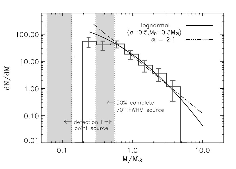
Figure 12: Differential mass distribution of all detected sources for masses calculated with $T_{D}=10$ K. The range in completeness, due to the range in local rms, is indicated by the shaded regions. The first is the range in detection limit for a point source, and the second is the range in 50% completeness limit for $70\arcsec$ FWHM sources, which is similar to the average source size of the sample. The best fitting power law ($\alpha=2.1$) is shown, as well as the best-fitting lognormal function.

Figure 12 shows the differential ($dN/dM$) core mass distribution (CMD) for the 44 secure detections. These include both starless cores and cores with protostars. The masses are taken from Table 2. Error bars in Figure 12 are $\sqrt{N}$ statistical errors only. The shaded regions on the figure represent the range in detection limit for a point source (left), and the 50% completeness limit for sources with a FWHM of $\sim 70\arcsec$ (right), which is approximately the average FWHM of the sample. We do not attempt to correct for incompleteness in the mass function. Most sources are found in the higher noise regions of the map; therefore the mass function is likely to be incomplete below 0.5 M_⊙.

The CMD above 0.5 M_⊙ can be fitted with either a power law (Salpeter, 1955), which gives a reduced chi-squared of $\mbox{$\chi_{r}^{2}$}=0.4$, or a lognormal function (Miller & Scalo, 1979), which gives $\mbox{$\chi_{r}^{2}$}=0.3$. The slightly better $\chi_{r}^{2}$ value for the lognormal function reflects the tendency of the distribution to flatten at lower masses, but incompleteness prevents us from distinguishing between these two functions. For the power law ($N(M)\propto M^{-\alpha}$), the best fit is for $\alpha=2.1\pm 0.3$. The lognormal distribution is given by

$$\frac{dN}{dlogM}=Aexp\left[\frac{-(logM-logM_{0})^{2}}{2\sigma_{M}^{2}}\right],$$ (4)

where $A$ is the normalization, $\sigma_{M}$ is the width of the distribution, and $M_{0}$ is the characteristic mass. The best-fitting lognormal function for $M>0.5$ M_⊙ has $\sigma_{M}=0.5\pm 0.4$ and $M_{0}=0.3\pm 0.7$ M_⊙.

The CMD depends on assumptions about distance, opacity, and dust temperature. Increasing the distance shifts it to higher masses, while increasing the opacity or dust temperature shifts it to lower masses. The CMDs in Perseus for four different dust temperatures ($T_{D}=5$, 10, 20, and 30 K) are shown in Figure 17 of Paper I. The distribution moves to lower masses for increasing temperature, but the overall shape of the distribution is not affected by changing $T_{D}$. However, if $T_{D}$ varies systematically with mass, the shape of the distribution could be changed. Experiments in which cores in the main cluster were given higher temperatures, or small cores were given higher temperatures produced little change in the mass distribution. If cores in the L1688 cluster were assigned $\mbox{$T_{D}$}=20$ K and other cores assigned $\mbox{$T_{D}$}=10$ K, the best-fit value became $\alpha=2.2$ for $M>0.5$ M_⊙, insignificantly different. However, the evidence for a turnover at low masses became even less significant. Such effects should be considered before inferring turnovers in CMDs.

Johnstone et al. (2000) (see their figure 7) fit the cumulative mass distribution for 850 µm cores within the L1688 region, assuming $\mbox{$T_{D}$}=20$ K, with a broken power law. They found $\alpha_{1}$ = 1.5 for masses less than about 0.6 M_⊙ and $\alpha_{2}$ = 2.5 for M $>0.6$ M_⊙. The Johnstone et al. (2000) sample is complete down to about $M\sim$ 0.4 M_⊙. If we assume $\mbox{$T_{D}$}=20$ K, the best-fit power law slope remains $\alpha=2.1$, but our completeness limit becomes 0.2 M_⊙. Thus, our mass function declines less rapidly than that of Johnstone et al. (2000), but the difference is not very significant. Since Johnstone et al. (2000) split some of our sources into multiple, smaller sources, it is natural that they would find a larger value of $\alpha$. Stanke et al. (2005) do not give a table of masses, but their CMD extends up to roughly 3 M_⊙, similar to our result, despite differences in source identification and mass calculation. They argue for breaks in their CMD around 0.2 and 0.7 M_⊙, with $\alpha\sim 2.6$ for large masses.

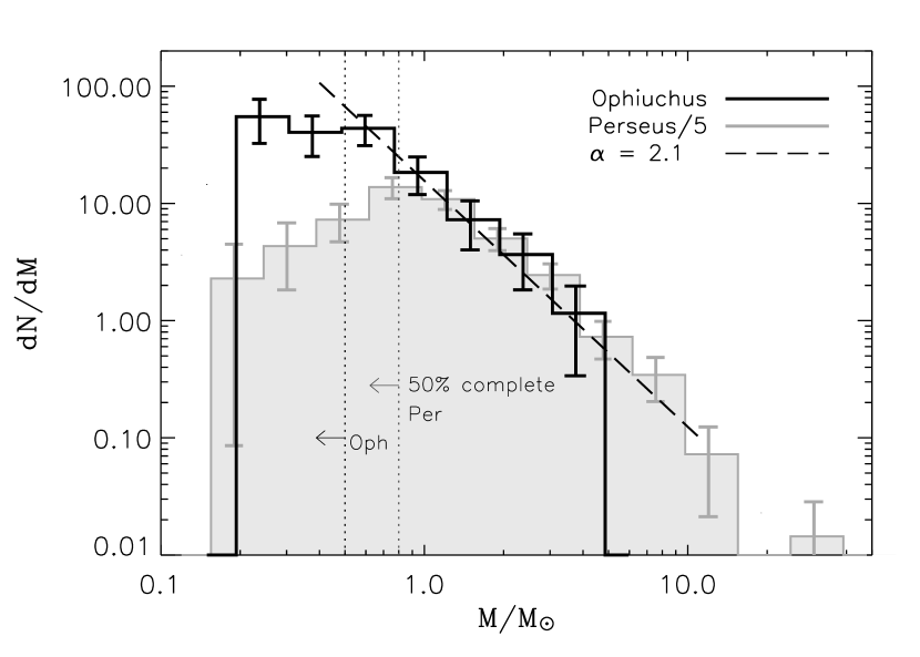
Figure 13: Comparison of the differential mass distributions of sources in Ophiuchus and Perseus (light line and gray-shaded). The Perseus mass function has been scaled by 1/5 to match the amplitude of the Ophiuchus distribution. Uncertainties reflect only the counting statistics ($\sqrt{N}$). Vertical dotted lines show the 50% completeness thresholds for 70″ FWHM sources for both clouds. The distributions appear quite similar in the region where both mass functions are complete.

The CMDs for Ophiuchus and Perseus are shown together for comparison in Figure 13, where the Perseus distribution has been scaled down by a factor of five to match the amplitude of the Ophiuchus mass function. In the region where both mass functions are reasonably complete ($M>0.8$ M_⊙), the two distributions appear quite similar except for the fact that the Ophiuchus mass function drops off at $\sim 4$ M_⊙ whereas the Perseus mass function extends to $M>10$ M_⊙. With a factor of 3 more sources in Perseus, statistical sampling of the same mass function naturally results in a higher maximum mass. The best single power-law fit ($\mbox{$\chi_{r}^{2}$}=0.8$) to the Perseus distribution for $M>0.8$ M_⊙ gave $\alpha=2.1\pm 0.15$, the same as the slope for Ophiuchus for $M>0.5$ M_⊙. Testi & Sargent (1998) also found $\alpha=2.1$ for a cluster in Serpens. Motte, André, & Neri (1998) found $\alpha=2.5$ above 0.5 M_⊙ for a broken power-law fit to cores in the Ophiuchus cluster, and Johnstone et al. (2000) found a similar result. Broken power-law fits tend to produce steeper slopes at higher masses, and the slopes are steeper if a higher break mass is assumed, suggesting that lognormal fits may be appropriate. The best lognormal fits to the Ophiuchus ($\sigma_{M}=0.5\pm 0.4$, $M_{0}=0.3\pm 0.7$ M_⊙) and Perseus ($\sigma_{M}=0.5\pm 0.1$, $M_{0}=0.9\pm 0.3$ M_⊙) mass functions have similar shapes within the uncertainties.

The CMD is most naturally compared to predictions from models of turbulent fragmentation in molecular clouds. Padoan & Nordlund (2002) argue that turbulent fragmentation naturally produces a power law with $\alpha=2.3$ (for the differential CMD that we plot). However, Ballesteros-Paredes et al. (2006) question this result, showing that the shape of the CMD depends strongly on Mach number in the turbulence. As the numerical simulations develop further, the observed CMD will provide a powerful observational constraint, with appropriate care in turning the simulations into observables.

The shape of the CMD may also be related to the process that determines final stellar masses. Assuming the simplest case in which a single process dominates the shape of the stellar initial mass function (IMF), the IMF should closely resemble the original CMD if stellar masses are determined by the initial fragmentation into cores (Adams & Fatuzzo, 1996). Alternatively, if stellar masses are determined by other processes, such as further fragmentation within cores, merging of cores, competitive accretion, or feedback, the IMF need not be related simply to the CMD (e.g., Ballesteros-Paredes et al. 2006).

In addition, the IMF itself is still uncertain (Scalo, 2006). For example, the Salpeter IMF would have $\alpha=2.35$ (Salpeter, 1955) in our plots. More recent work on the local IMF finds evidence for a break in the slope around 1 M_⊙. The slope above the break depends on the choice of break mass. For example, Reid et al. (2002) find $\alpha=2.5$ above 0.6 M_⊙, and $\alpha=2.8$ above 1 M_⊙. Chabrier (2003) suggests $\alpha=2.7$ ($M>1$ M_⊙), while Schröder & Pagel (2003) finds $\alpha=2.7$ for $1.1<M_{\star}<1.6$ M_⊙and $\alpha=3.1$ for $1.6<M_{\star}<4$ M_⊙. Given the uncertainties and the differences between fitting single and broken power laws, all these values for $\alpha$ are probably consistent with each other and with determinations of the CMD.

Currently, we cannot separate prestellar cores from more evolved objects in either Perseus or Ophiuchus, so a direct connection to the IMF is difficult to make. After combining these data with Spitzer data it will be possible to determine the evolutionary state of each source and compare the mass function of prestellar cores only. Further comparisons of clustering properties and the probability of detecting cores as a function of $A_{V}$ in Ophiuchus and Perseus are discussed in the following sections.

5.3 Clustering

The majority of the sources detected with Bolocam in Ophiuchus are very clustered. Of the 44 sources, 36 are multiple (Table 2), with a neighboring source within 3′, corresponding to 22,500 AU at a distance of 125 pc. The average separation for the whole sample is 153″, or 19000 AU. If we consider only sources in the L1688 region for comparison to previous studies, the mean separation is $116\arcsec$, or 14500 AU. The median separation in L1688 is substantially smaller ($69\arcsec=8600$ AU). The median separation in L1688 is very similar to the mean size of the sources in the sample, 68″, as determined by averaging the major and minor FWHM. This indicates that many source pairs are barely resolved. It also means that the measured size of many sources is limited to something like the mean separation, since the Gaussian fitting routine takes into account the distance to the nearest neighbor when determining source size.

The median separation of 8600 AU for the L1688 cluster is only slightly larger than the fragmentation scale of 6000 AU suggested by Motte, André, & Neri (1998) in their study of the main Ophiuchus cluster by examining the mean separation between cores in their data. Resolution effects likely play a role here, as our resolution (3900 AU) is approximately twice that of Motte, André, & Neri (1998). Stanke et al. (2005) find two peaks in the distribution of source separations of neighboring cores ($\sim 5000$ AU and $\sim 13000$ AU), suggesting that they also distinguish the cores in the Ophiuchus cluster from those in the more extended cloud. The median core separation is still smaller than the median separation of T Tauri stars in Taurus of 50000 AU (Gomez et al., 1993) as pointed out by Motte, André, & Neri (1998).

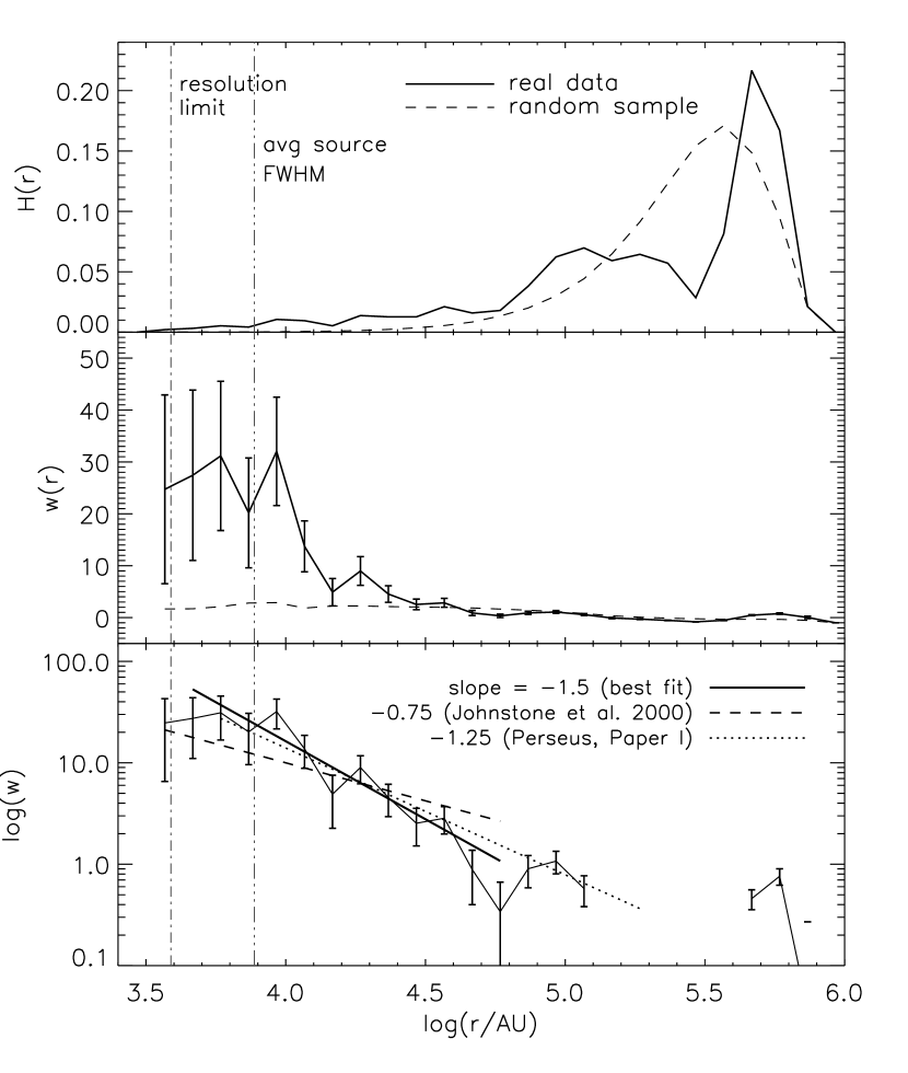
Figure 14: Top: $H(r)$, the fractional number of source pairs between log($r$) and dlog($r$), versus log($r$). The solid line indicates the real data, and the dashed line is for a uniform random distribution of sources with the same RA/Dec limits as the real sample. In all plots, the resolution limit and the average source FWHM are shown. Middle: Two-point correlation function, with $\sqrt{N}$ errors. Bottom: Log of the correlation function with power-law fits. The best fit slope is $-1.5\pm 0.3$. The slope found by Johnstone et al. (2000) in Ophiuchus is shallower ($-0.75$), while the slope found in Perseus in Paper I was similar ($-1.25\pm 0.06$).

Another description of source clustering is provided by the two-point correlation function, as was used in Paper I and Johnstone et al. (2000). Figure 14 plots $H(r)$, $w(r)$, and log($w(r)$) versus the log of the distance between sources, $r$. $H(r)$ is the fractional number of source pairs with a separation between log($r$) and log($r$) + dlog($r$) and is plotted both for the Ophiuchus sources ($H_{s}(r)$; solid lines in Figure 14) and for a uniform random distribution of sources ($H_{r}(r)$; dashed lines) with the same observational RA and Dec limits as the real sample (i.e. there are no sources in the random sample outside the actual area observed). Because it is discontinuous from the rest of the map, the northeastern streamer is not included in this analysis. $w(r)$ is the two-point correlation function, given by the equation:

$$w(r)=\frac{H_{s}(r)}{H_{r}(r)}-1.$$ (5)

The top panel of Figure 14 shows an excess in $H_{s}(r)$ over the random sample $H_{r}(r)$ for small separations. The excess indicates that the sources in Ophiuchus are not randomly distributed within the cloud, but clustered on small scales. The middle panel shows that the two-point correlation function for the Ophiuchus data exceeds zero by 2.5 $\sigma$ for $r<4\times 10^{4}$ AU, but the random distribution shows no correlation ($w(r)=0$). The bottom panel of the figure shows that the correlation function can be fit with a power law, $w\propto r^{-\gamma}$; the best fit gives $\gamma=1.5\pm 0.3$ ($\mbox{$\chi_{r}^{2}$}=1.2$) for $1\times 10^{4}$ AU $<r<4\times 10^{4}$ AU. The correlation function for Perseus was characterized by $\gamma=1.25\pm 0.06$ ($\mbox{$\chi_{r}^{2}$}=0.7$) for $2\times 10^{4}$ AU $<r<2\times 10^{5}$ AU.

Stanke et al. (2005) found $\gamma=0.63$ out to $r\sim 1\mbox{${}\times 10^{5}$}$ AU. Johnstone et al. (2000) also fitted the correlation for the Ophiuchus cluster with a shallower power law, $\gamma=0.75$ for $r<3\times 10^{4}$ in the L1688 cluster region of Ophiuchus. This power law is also shown in Figure 14, but it clearly does not fit our data. Johnstone et al. (2000) were able to measure the correlation function to smaller scales, $r=4.5\times 10^{3}$ AU, than this study, which may result in some discrepancy in the best-fit power law between the two data sets. The correlation function does appear flatter for smaller separations, but the slope may be complicated by blending for small separations. If the correlation function is restricted to sources in the L1688 cluster, the slope becomes more consistent with those found by Johnstone et al. (2000) and Stanke et al. (2005).

We conclude from this analysis that the sources in Ophiuchus are clearly clustered. Determining the parameters of the correlation function is complicated by effects of map size and resolution.

5.4 Extinction threshold

Johnstone, Di Francesco, & Kirk (2004) suggested that there is a threshold at $A_{V}=15$ mag in Ophiuchus for the formation of cores, with 94% of the mass in cores found at or above that extinction level. They did see cores below that level, but they were faint (low peak flux) and low in mass (low total flux). They mapped 4 square degrees of Ophiuchus at 850 µm and compared their data to an extinction map of Ophiuchus created from 2MASS and R-band data as part of the COMPLETE project. Comparison of our own extinction map (Fig. 6) with the COMPLETE extinction map shows reasonable agreement, so we use our extinction map.

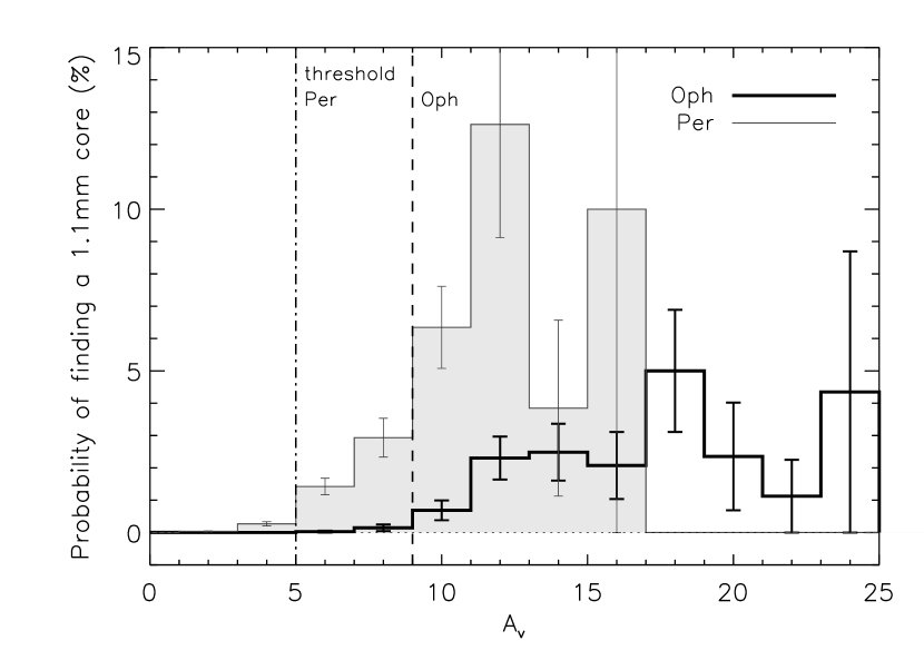
Figure 15: Probability of finding a 1.1 mm core as a function of $A_{V}$. The probability is the number of 50″ pixels at a given $A_{V}$ containing one or more 1.1 mm cores, divided by the total number of pixels at that $A_{V}$. Error bars are Poisson statistical errors. The dashed vertical line shows our proposed threshold at $A_{V}=9$ mag. The probability distribution for Perseus (light line and gray-shaded) from Paper I is also shown for comparison, with the dash-dotted line showing the threshold in Perseus.

We have used a simple analysis, comparable to that of Hatchell et al. (2005), to study the extinction threshold. Figure 15 plots the probability of finding a 1.1 mm core in Ophiuchus as a function of $A_{V}$. The probability for a given $A_{V}$ is calculated from the extinction map as the number of 50″ pixels containing a 1.1 mm core divided by the total number of pixels at that $A_{V}$, and error bars are Poisson statistical errors.

Very few sources are found below $A_{V}=9$ mag; 93% of the mass in cores is found above $\mbox{$A_{V}$}=8$ mag (see Table 3). Thus we suggest that $\mbox{$A_{V}$}=9$ mag is the extinction limit for finding 1.1 mm cores in Ophiuchus. The probability of finding a core increases with $A_{V}$ beyond this point, although the uncertainties are large at high $A_{V}$ because there are few pixels in the extinction map at very high extinctions. The probability distribution for Perseus from Paper I is also shown for comparison. The difference is quite striking; Perseus seems to have a much lower extinction threshold than does Ophiuchus, even as measured by us, and still lower than the threshold for Ophiuchus found by Johnstone, Di Francesco, & Kirk (2004).

To explore the issues further, we plot in Figure 16 total flux density, peak flux density, radius, and mass for $T_{D}=10$ K versus $A_{V}$. In contrast to the Johnstone, Di Francesco, & Kirk (2004) study, we find many (12 out of the total core sample of 44) bright (total flux density $>$ 3 Jy) and massive ($M$(10 K) $>$ 2 M_⊙) sources at $A_{V}<$ 15 mag. Conclusions about thresholds depend on sensitivity to large structures, slight differences in extinction contours, and differing resolution. For example, the tentative detections listed in Table 1 are in regions with $\mbox{$A_{V}$}<9$.

The areas and cloud masses, measured from the extinction, above contours of $A_{V}$ are given in Table 3, along with the masses of cores above the same contours. The percentages of the total cloud and core masses are also given. Finally, the fraction of the cloud mass that is found in dense cores, measured for the same contour level, is given in the last column. This is similar to Table 2 of Johnstone, Di Francesco, & Kirk (2004), except that our cloud and core masses are cumulative and we use bins of $\mbox{$A_{V}$}=2$ mag. Even with our lower threshold, nearly half the total core mass lies above the $\mbox{$A_{V}$}=14$ mag contour, which occupies only 2.3% of the cloud area and 10% of the cloud mass. The dense cores are clearly concentrated in the regions of high extinction. The ratio of core to cloud mass increases from about 2% at the lowest contour ($\mbox{$A_{V}$}=2$) to an average of 7.4% for contours between 8 and 18 mag. (The contour above 20 mag has such little area that the core mass fraction is not very reliable.)

6 Summary

We presented a 1.1 mm dust continuum emission map of 10.8 deg² of the Ophiuchus molecular cloud. We detected 44 sources at 4 $\sigma$ or greater, almost all concentrated around well known clusters (near the dark clouds L1688, L1689, and L1709). Some weaker emission (3 $\sigma$) was seen along the eastern streamer of the cloud, coincident with a filament seen in both extinction (Fig. 6) and emission at 160 µm (Fig. 5). These cores have been previously seen in maps of CO, but these are the first millimeter dust continuum observations of the streamer. We did not detect any emission in the northeastern streamer.

Visually, the 4-$\sigma$ sources appear highly clustered, and this impression is confirmed by the two-point correlation function, the fraction of multiple sources, and the median separation. Fully 82% of the sources are classified as multiple (i.e., another source lies within 3′). Most of the cloud area has no detectable sources.

Most sources are round as measured at the FWHM, but many are elongated when measured at lower contour levels. This difference probably reflects the fact that many are relatively spherical condensations within filaments. Filamentary structure with condensations along the filaments is the dominant morphological theme.

The total mass of the sources is only 42 M_⊙, about 0.4 to 1.8% of the total cloud mass, lower than in Perseus (Paper I), while the total mass corresponding to emission above 4 $\sigma$ is 79 M_⊙. The differential mass distribution can be fitted with a power law with slope $-2.1\pm 0.3$ or a lognormal function. It is similar to that in Perseus, but does not extend to as high a mass, with the most massive core containing only 3.9 M_⊙. The mean densities are quite high, averaging $1.6\mbox{${}\times 10^{6}$}$ cm^-3, implying a short free-fall time.

Millimeter continuum sources are seen for $A_{V}$ above a threshold value of 9 mag, higher than in Perseus, but lower than found in previous studies of Ophiuchus by Johnstone, Di Francesco, & Kirk (2004). About half the total mass of dense cores are in contours of extinction below $A_{V}=14$ mag, near the threshold seen by Johnstone, Di Francesco, & Kirk (2004). Still, the cores are clearly concentrated in a small fraction of the cloud area and mass, and in regions of relatively high extinction.

Future analysis of these data in combination with the c2d Spitzer maps of Ophiuchus will give a more complete picture of star formation in the cloud. Additionally, the environments of other clouds in the c2d survey will be compared using the combined infrared and millimeter data sets in future work.

Table 1: Sources Found in Ophiuchus

ID	RA (2000)	Dec (2000)	Peak	S/N	other names
	($h~{}~{}m~{}~{}s$)	($\arcdeg~{}~{}\arcmin~{}~{}\arcsec$)	(Jy/beam)
Bolo 1	16 25 59.1	-24 18 16.2	0.26 (0.03)	4.5
Bolo 2	16 26 08.1	-24 20 00.6	0.39 (0.03)	4.7	CRBR 2305.4-1241 ?
Bolo 3	16 26 09.6	-24 19 15.6	0.31 (0.03)	4.1	SMM J16261-2419 (1)
Bolo 4	16 26 09.9	-24 20 28.6	0.40 (0.03)	6.2	GSS26?
Bolo 5	16 26 20.7	-24 22 17.0	0.37 (0.04)	4.3	GSS30-IRS3 (2); SMM J16263-2422 (1); LFAM1 (3)
Bolo 6	16 26 22.9	-24 20 00.9	0.27 (0.03)	4.5	SMM J16263-2419 (1)
Bolo 7	16 26 24.7	-24 21 07.5	0.41 (0.04)	4.9	A-MM4? (5)
Bolo 8	16 26 27.2	-24 22 26.7	1.38 (0.04)	16.0	SM1 FIR1 (4); A-MM5/6?? (5); SMM J16264-2422 (1)
Bolo 9	16 26 27.6	-24 23 36.6	2.70 (0.04)	45.2	SM1 FIR2 (4); SM1N
Bolo 10	16 26 29.7	-24 24 28.8	2.66 (0.04)	47.5	SM2
Bolo 11	16 26 32.6	-24 24 45.3	1.25 (0.04)	14.8	A-MM8 (5)
Bolo 12	16 27 00.7	-24 34 17.0	0.54 (0.03)	8.4	SMM J16269-2434 (1); C-MM3 (5)
Bolo 13	16 27 04.3	-24 38 47.4	0.23 (0.03)	4.8	E-MM2d (5); SMM J16270-2439 (1)
Bolo 14	16 27 07.9	-24 36 54.3	0.26 (0.03)	4.4	SMM J16271-2437a/b (1); Elias29?
Bolo 15	16 27 12.2	-24 29 18.9	0.44 (0.04)	6.1	B1-MM2/3 (5); IRAS 16242-2422; SMM J16272-2429 (1)
Bolo 16	16 27 15.1	-24 30 12.6	0.45 (0.04)	7.1	SMM J16272-2430 (1); B1-MM4 (5)
Bolo 17	16 27 22.3	-24 27 36.3	0.40 (0.04)	4.4	B2-MM4 (5)
Bolo 18	16 27 25.2	-24 40 28.9	0.47 (0.03)	9.7	F-MM2 (5); IRS43? (5)
Bolo 19	16 27 27.0	-24 26 57.1	0.62 (0.04)	7.4	SMM J16274-2427s (1)
Bolo 20	16 27 29.1	-24 27 11.1	0.69 (0.04)	9.4	B2-MM8 (5); SMM J16274-2427b (1)
Bolo 21	16 27 33.1	-24 26 48.8	0.53 (0.04)	6.8	B2-MM15 (5); SMM J16275-2426 (1)
Bolo 22	16 27 33.4	-24 25 57.3	0.50 (0.03)	9.4	B2-MM13 (5); SMM J16275-2426 (1)
Bolo 23	16 27 36.7	-24 26 36.2	0.40 (0.03)	5.1	B2-MM17 (5)
Bolo 24	16 27 58.3	-24 33 09.7	0.29 (0.03)	6.0
Bolo 25	16 28 00.1	-24 33 42.8	0.33 (0.03)	6.0	H-MM1 (8)
Bolo 26	16 28 21.0	-24 36 00.0	0.23 (0.03)	5.5
Bolo 27	16 28 32.1	-24 17 43.4	0.17 (0.03)	4.1	D-MM3/4 (5)
Bolo 28	16 28 57.7	-24 20 33.7	0.28 (0.03)	5.8	I-MM1 (8)
Bolo 29	16 31 36.4	-24 00 41.7	0.28 (0.03)	7.0	L1709-SMM1 (6); IRS63
Bolo 30	16 31 37.2	-24 01 51.9	0.29 (0.03)	6.3	L1709-SMM3,5 (6)
Bolo 31	16 31 40.0	-24 49 58.0	0.45 (0.03)	6.8
Bolo 32	16 31 40.4	-24 49 26.4	0.45 (0.03)	7.4
Bolo 33	16 31 52.6	-24 58 00.8	0.20 (0.03)	4.5
Bolo 34	16 31 58.0	-24 57 38.8	0.26 (0.03)	5.2
Bolo 35	16 32 00.6	-24 56 13.9	0.19 (0.03)	4.5	IRAS 16289-2450; L1689S; IRS67
Bolo 36	16 32 22.5	-24 27 47.5	1.65 (0.03)	17.9
Bolo 37	16 32 24.7	-24 28 51.2	3.03 (0.03)	80.7	IRAS 16293-2422
Bolo 38	16 32 28.6	-24 28 37.5	1.07 (0.03)	17.0
Bolo 39	16 32 30.1	-23 55 18.4	0.25 (0.03)	4.8	L1709-SMM2 (6)
Bolo 40	16 32 30.8	-24 29 28.3	0.74 (0.03)	14.7
Bolo 41	16 32 42.3	-24 31 13.0	0.15 (0.02)	4.5
Bolo 42	16 32 44.1	-24 33 21.6	0.20 (0.03)	4.3
Bolo 43	16 32 49.2	-23 52 33.9	0.28 (0.03)	4.1	L1709-SMM4? (6); LM182
Bolo 44	16 34 48.3	-24 37 24.6	0.21 (0.02)	5.6	L1689B-3
Tentative detections in the eastern streamer
Bolo 45	16 38 07.8	-24 16 36.4	0.15 (0.02)	3.6	$\rho$-Oph 10 (7)
Bolo 46	16 39 15.8	-24 12 20.8	0.10 (0.02)	3.2
Bolo 47	16 41 44.5	-24 05 20.4	0.14 (0.02)	3.0
Bolo 48	16 41 55.6	-24 05 41.6	0.12 (0.02)	3.0

Note. — Numbers in parentheses are $1\sigma$ errors. The peak flux density is the peak pixel value in the $10\arcsec$ pixel^-1 unfiltered map (without the Wiener filter applied). The uncertainty in the peak flux density is the local (calculated within a 400″ box) rms beam^-1, calculated from the noise map, and does not include an additional 15% systematic uncertainty from calibration uncertainties and residual errors after iterative mapping. Other names listed are the most common identifications from the literature, and are not meant to be a complete list. References – (1) Johnstone et al. 2000; (2) Castelaz et al. 1985, Weintraub et al. 1993; (3) Leous et al. 1991; (4) Mezger et al. 1992; (5) Motte, Andre & Neri 1998; (6) Visser et al. (2002); (7) Tachihara, Mizuno, & Fukui (2000); (8) Johnstone, Di Francesco, & Kirk (2004)

Table 2: Photometry and Core Properties

ID	Flux($40\arcsec$)	Flux($80\arcsec$)	Flux($120\arcsec$)	Total Flux	Mass (10K)	Peak $A_{V}$	FWHM	FWHM	PA	$\langle n\rangle$	Morphology
	(Jy)	(Jy)	(Jy)	(Jy)	($M_{\sun}$)	(mag)	(minor,$\arcsec$)	(major,$\arcsec$)	($\arcdeg$)	cm-3
Bolo1	0.34 (0.03)	0.82 (0.07)	1.55 (0.1)	2.13 (0.13)	1.29 (0.08)	18	88 (0.9)	133 (1.4)	-24 (2)	2$\times 10^{5}$	multiple,extended,round
Bolo2	$\cdots$	$\cdots$	$\cdots$	0.46 (0.03)	0.28 (0.02)	27	55 (0.6)	58 (0.6)	29 (17)	4$\times 10^{5}$	multiple,round
Bolo3	0.46 (0.04)	$\cdots$	$\cdots$	0.58 (0.05)	0.35 (0.03)	22	53 (0.7)	58 (0.8)	88 (10)	5$\times 10^{5}$	multiple,extended,round
Bolo4	$\cdots$	$\cdots$	$\cdots$	0.49 (0.03)	0.3 (0.02)	28	52 (0.6)	56 (0.7)	-10 (11)	5$\times 10^{5}$	multiple,elongated
Bolo5	0.55 (0.05)	1.32 (0.1)	$\cdots$	1.61 (0.11)	0.97 (0.07)	26	64 (0.8)	70 (0.8)	26 (11)	7$\times 10^{5}$	multiple,extended,elongated
Bolo6	0.32 (0.05)	$\cdots$	$\cdots$	0.58 (0.08)	0.35 (0.05)	19	59 (1.3)	67 (1.5)	-61 (14)	3$\times 10^{5}$	multiple,extended,weak
Bolo7	0.56 (0.05)	$\cdots$	$\cdots$	1.08 (0.08)	0.65 (0.05)	29	56 (0.6)	66 (0.8)	-50 (6)	7$\times 10^{5}$	multiple,extended,elongated
Bolo8	1.86 (0.05)	$\cdots$	$\cdots$	3.93 (0.09)	2.37 (0.05)	98	55 (0.2)	63 (0.2)	81 (2)	3$\times 10^{6}$	multiple,extended,round
Bolo9	4.2 (0.05)	$\cdots$	$\cdots$	6.49 (0.08)	3.92 (0.05)	191	46 (0.1)	56 (0.1)	-68 (1)	9$\times 10^{6}$	multiple,extended,round
Bolo10	3.42 (0.05)	$\cdots$	$\cdots$	3.42 (0.05)	2.07 (0.03)	189	44 (0.1)	56 (0.1)	22 (1)	5$\times 10^{6}$	multiple,extended,round
Bolo11	1.72 (0.05)	$\cdots$	$\cdots$	1.72 (0.05)	1.04 (0.03)	88	49 (0.2)	54 (0.2)	50 (3)	2$\times 10^{6}$	multiple,extended,round
Bolo12	0.86 (0.04)	2.11 (0.09)	3.91 (0.13)	5.56 (0.17)	3.36 (0.1)	38	105 (0.5)	125 (0.6)	-45 (2)	4$\times 10^{5}$	extended,elongated
Bolo13	0.35 (0.04)	0.75 (0.08)	1.35 (0.12)	1.35 (0.12)	0.82 (0.07)	16	76 (1.2)	96 (1.5)	44 (5)	2$\times 10^{5}$	multiple,extended,elongated,weak
Bolo14	0.32 (0.05)	0.68 (0.09)	1.19 (0.14)	1.19 (0.14)	0.72 (0.08)	18	66 (1.2)	108 (2.)	41 (3)	2$\times 10^{5}$	multiple,extended,weak
Bolo15	0.61 (0.05)	$\cdots$	$\cdots$	0.92 (0.07)	0.56 (0.04)	31	50 (0.7)	64 (0.8)	19 (4)	8$\times 10^{5}$	multiple,extended,elongated
Bolo16	0.7 (0.05)	$\cdots$	$\cdots$	1.08 (0.07)	0.65 (0.04)	32	51 (0.6)	62 (0.7)	-58 (5)	9$\times 10^{5}$	multiple,extended,elongated
Bolo17	0.54 (0.05)	$\cdots$	$\cdots$	1.03 (0.09)	0.62 (0.06)	29	56 (0.8)	68 (1.)	-62 (6)	6$\times 10^{5}$	multiple,extended,elongated
Bolo18	0.65 (0.04)	1.49 (0.08)	2.64 (0.11)	3.76 (0.15)	2.27 (0.09)	33	96 (0.6)	149 (1.)	41 (1)	2$\times 10^{5}$	extended,elongated
Bolo19	$\cdots$	$\cdots$	$\cdots$	0.8 (0.04)	0.48 (0.02)	44	54 (0.4)	58 (0.4)	-8 (9)	7$\times 10^{5}$	multiple,round
Bolo20	$\cdots$	$\cdots$	$\cdots$	0.87 (0.04)	0.53 (0.02)	49	51 (0.4)	57 (0.4)	80 (6)	9$\times 10^{5}$	multiple,extended,round
Bolo21	0.82 (0.04)	$\cdots$	$\cdots$	1.01 (0.06)	0.61 (0.03)	37	53 (0.5)	60 (0.5)	40 (5)	9$\times 10^{5}$	multiple,extended,round
Bolo22	0.77 (0.04)	$\cdots$	$\cdots$	0.96 (0.06)	0.58 (0.03)	35	54 (0.5)	55 (0.5)	-75 (61)	10$\times 10^{5}$	multiple,extended,elongated
Bolo23	0.55 (0.04)	$\cdots$	$\cdots$	0.68 (0.05)	0.41 (0.03)	28	53 (0.6)	56 (0.7)	-88 (20)	7$\times 10^{5}$	multiple,extended,round
Bolo24	0.39 (0.04)	$\cdots$	$\cdots$	0.39 (0.04)	0.24 (0.02)	21	48 (0.8)	57 (0.9)	14 (7)	5$\times 10^{5}$	multiple,extended,elongated
Bolo25	0.39 (0.04)	$\cdots$	$\cdots$	0.39 (0.04)	0.24 (0.02)	23	47 (0.8)	56 (0.9)	-66 (7)	5$\times 10^{5}$	multiple,elongated
Bolo26	0.3 (0.03)	0.63 (0.07)	1.14 (0.1)	1.62 (0.14)	0.98 (0.08)	16	108 (1.4)	132 (1.8)	84 (5)	9$\times 10^{4}$	extended,elongated
Bolo27	0.23 (0.03)	0.52 (0.07)	0.97 (0.1)	1.48 (0.13)	0.9 (0.08)	12	89 (1.1)	157 (2.)	58 (2)	9$\times 10^{4}$	extended,elongated,weak
Bolo28	0.37 (0.03)	0.86 (0.07)	1.55 (0.1)	2.17 (0.13)	1.31 (0.08)	20	102 (1.)	113 (1.1)	74 (8)	2$\times 10^{5}$	extended,elongated
Bolo29	0.28 (0.04)	$\cdots$	$\cdots$	0.5 (0.07)	0.3 (0.04)	20	54 (1.)	57 (1.1)	11 (29)	5$\times 10^{5}$	multiple,extended,elongated
Bolo30	0.28 (0.04)	$\cdots$	$\cdots$	0.46 (0.06)	0.28 (0.04)	20	46 (1.1)	57 (1.3)	66 (9)	6$\times 10^{5}$	multiple,extended,elongated
Bolo31	$\cdots$	$\cdots$	$\cdots$	0.55 (0.03)	0.33 (0.02)	32	54 (0.5)	57 (0.5)	-61 (15)	5$\times 10^{5}$	multiple,round
Bolo32	$\cdots$	$\cdots$	$\cdots$	0.53 (0.03)	0.32 (0.02)	31	56 (0.5)	58 (0.5)	74 (20)	4$\times 10^{5}$	multiple,round
Bolo33	0.26 (0.04)	0.57 (0.07)	$\cdots$	0.57 (0.07)	0.35 (0.04)	14	54 (1.2)	65 (1.5)	-33 (10)	4$\times 10^{5}$	multiple,extended,elongated,weak
Bolo34	0.38 (0.04)	0.87 (0.08)	$\cdots$	0.87 (0.08)	0.52 (0.05)	19	59 (0.9)	68 (1.1)	-73 (9)	4$\times 10^{5}$	multiple,extended,elongated
Bolo35	0.22 (0.04)	0.39 (0.08)	$\cdots$	0.46 (0.09)	0.28 (0.06)	13	66 (1.7)	77 (2.1)	40 (14)	2$\times 10^{5}$	multiple,extended,elongated,weak
Bolo36	1.35 (0.04)	$\cdots$	$\cdots$	2.49 (0.07)	1.51 (0.04)	117	53 (0.2)	57 (0.2)	-17 (5)	2$\times 10^{6}$	multiple,extended,round
Bolo37	3.63 (0.04)	$\cdots$	$\cdots$	4.47 (0.06)	2.7 (0.04)	214	35 (0.1)	45 (0.1)	49 (1)	3$\times 10^{7}$	multiple,round
Bolo38	1.52 (0.04)	$\cdots$	$\cdots$	2.33 (0.06)	1.41 (0.04)	76	54 (0.2)	54 (0.2)	-15 (38)	2$\times 10^{6}$	multiple,extended,round
Bolo39	0.26 (0.04)	0.55 (0.07)	0.94 (0.11)	1.29 (0.14)	0.78 (0.08)	17	101 (1.7)	128 (2.2)	-51 (6)	9$\times 10^{4}$	extended
Bolo40	1.11 (0.04)	$\cdots$	$\cdots$	1.67 (0.06)	1.01 (0.04)	52	49 (0.3)	58 (0.3)	55 (3)	2$\times 10^{6}$	multiple,extended,round
Bolo41	0.2 (0.03)	0.39 (0.06)	0.73 (0.09)	0.85 (0.1)	0.51 (0.06)	11	40 (1.2)	53 (1.6)	-27 (9)	2$\times 10^{6}$	multiple,extended,elongated,weak
Bolo42	0.19 (0.03)	0.39 (0.07)	0.72 (0.1)	0.83 (0.11)	0.5 (0.07)	14	53 (1.6)	66 (1.9)	80 (11)	6$\times 10^{5}$	multiple,extended,elongated,weak
Bolo43	0.33 (0.04)	0.84 (0.07)	1.63 (0.11)	2.45 (0.15)	1.48 (0.09)	20	98 (0.9)	143 (1.3)	47 (2)	1$\times 10^{5}$	extended,elongated
Bolo44	0.3 (0.03)	0.72 (0.06)	1.21 (0.09)	1.71 (0.12)	1.03 (0.08)	15	96 (1.1)	119 (1.4)	55 (4)	1$\times 10^{5}$	extended,round
Tentative detections in the eastern streamer
Bolo45	0.20 (0.03)	0.47 (0.06)	0.94 (0.09)	1.36 (0.11)	0.82 (0.06)	11	123 (1.5)	157 (1.9)	-51 (4)	5$\times 10^{4}$	extended,elongated,weak
Bolo46	$\cdots$	$\cdots$	$\cdots$	0.08 (0.02)	0.05 (0.01)	7	64 (3)	153 (6)	7 (3)	9$\times 10^{3}$	extended,round,weak
Bolo47	0.13 (0.03)	$\cdots$	$\cdots$	0.15 (0.04)	0.09 (0.02)	10	87 (2)	112 (3)	-42 (9)	2$\times 10^{4}$	multiple,extended,round,weak
Bolo48	$\cdots$	$\cdots$	$\cdots$	0.86 (0.13)	0.52 (0.08)	8	84 (2)	111 (3)	-8 (7)	1$\times 10^{5}$	multiple,extended,round,weak

Note. — Masses are calculated according to Equation 1 from the total flux density assuming a single dust temperature of $T_{D}=10K$ and a dust opacity at 1.1mm of $\kappa_{1.1mm}=0.0114$ cm²g^-1. Peak $A_{V}$ is calculated from the peak flux density as in Equation 2. FWHM and PAs are from a Gaussian fit; the PA is measured in degrees east of north of the major axis. $\langle n\rangle$ is the mean particle density as calculated from the total mass and the deconvolved average FWHM size. Numbers in parentheses are $1\sigma$ uncertainties. Uncertainties for masses are from photometry only, and do not include uncertainties from $\kappa$, $T_{D}$, or $d$, which can be up to a factor of a few or more. Uncertainties for the FWHM and PA are formal fitting errors from the elliptical Gaussian fit; additional uncertainties of $10-15$% apply to the FWHM, and $\sim 5\arcdeg$ to the PA (determined from simulations).

Table 3: Cumulative Mass as a Function of Extinction

Min. $A_{V}$	Area	Cloud Mass	Percent	Core Mass	Percent	Mass Ratio
mag	(%)	(M⊙)	(%)	(M⊙)	(%)	(%)
2	100	2300	100	42	100	1.8
4	39	1500	65	42	100	2.8
6	17	920	40	42	100	4.6
8	8.8	640	28	39	93	6.1
10	5.5	470	20	37	88	7.9
12	3.8	350	15	33	79	9.4
14	2.3	240	10	20	47	8.3
16	1.4	170	7.4	12	29	7.1
18	0.9	120	5.2	6.4	15	5.3
20	0.5	73	3.1	1.2	2.9	1.6

Note. — Cloud areas and masses are calculated from the extinction and conversions from §4.2.3. Core masses are taken from Table 2.

Figure 8: The distribution of source FWHM minor axis (dashed line) and major axis (solid line), as determined from an elliptical Gaussian fit. The beam size is indicated by the dotted line. The mean FWHM sizes of the sample are $62\arcsec$ (minor) and $77\arcsec$ (major). The top axis gives deconvolved sizes in AU, assuming a $31^{\prime\prime}$ beam and $d=125$ pc.

Figure 16: 1.1 mm source properties versus $A_{V}$. The dotted vertical lines are the $A_{V}=15$ mag threshold proposed by Johnstone, Di Francesco, & Kirk (2004). The solid vertical line is the $A_{V}$ = 9 mag extinction threshold from Figure 15. The dashed horizontal lines are the beam size in the upper right panel and the average 4-$\sigma$ detection limit in the lower left panel.

References

- Adams & Fatuzzo (1996) Adams, F. C., & Fatuzzo, M. 1996, ApJ, 464, 256
- Allen et al. (2002) Allen, L. E., Myers, P. C., DiFrancesco, J., Matheiu, R., Chen, H., & Young, E. 2002, ApJ, 566, 993
- Ballesteros-Paredes et al. (2006) Ballesteros-Paredes, J., Gazol, A., Kim, J., Klessen, R. S., Jappsen, A.-K., & Tejero, E. 2006, ApJ, 637, 384
- Bohlin et al. (1978) Bohlin, R. C., Savage, B. D., & Drake, J. F. 1978, ApJ, 224, 132
- Chabrier (2003) Chabrier, G. 2003, PASP, 115, 763
- Cambrésy (1999) Cambrésy, L. 1999, A&A, 345, 965
- Castelaz et al. (1985) Castelaz, M. W., Gehrz, R. D., Grasdalen, G. L., & Hackwell, J. A. 1985, PASP, 97, 924
- de Geus, de Zeeuw, & Lub (1989) de Geus, E. J., de Zeeuw, P. T., Lub, J. 1989, A&A, 216, 44
- Enoch et al. (2006) Enoch, M. L. et al. 2006, ApJ, in press (astro-ph/0510202)
- Evans (1999) Evans, N. J. 1999, ARA&A, 37, 311
- Evans et al. (2003) Evans, N. J., II, et al. 2003, PASP, 115, 965
- Glenn et al. (2003) Glenn, Jason; Ade, Peter A. R.; Amarie, Mihail; Bock, James J.; Edgington, Samantha F.; Goldin, Alexey; Golwala, Sunil; Haig, Douglas; Lange, Andrew E.; Laurent, Glenn; Mauskopf, Philip D.; Yun, Minhee; Nguyen, Hien, Millimeter and Submillimeter Detectors for Astronomy. Edited by Phillips, Thomas G.; Zmuidzinas, Jonas. Proceedings of the SPIE, Volume 4855, pp. 30-40 (2003)
- Gomez et al. (1993) Gomez, M., Hartmann, L., Kenyon, S. J., & Hewett, R. 1993, AJ, 105, 1927
- Goodman (2004) Goodman, A. A., 2004, in Star Formation in the Interstellar Medium (San Francisco: ASP), in press, http://cfa-www.harvard.edu/COMPLETE
- Hatchell et al. (2005) Hatchell, J., Richer, J. S., Fuller, G. A., Qualtrough, C. J., Ladd, E. F., & Chandler, C. J. 2005, A&A, 440, 151
- Huard et al. (2006) Huard, T. L., et al. 2006, ApJ, 640, in press
- Imanishi et al. (2001) Imanishi, K, Koyama, K., Tsuboi, Y. 2001, ApJ, 557, 747