Young, Low-mass Brown Dwarfs with Mid-Infrared Excesses

Abstract

We have combined new I, J, H, and Ks imaging of portions of the Chamaeleon II, Lupus I, and Ophiuchus star-forming clouds with with 3.6 to 24 $\mu$m imaging from the Spitzer Legacy Program, “From Molecular Cores to Planet Forming Disks”, to identify a sample of 19 young stars, brown dwarfs and sub-brown dwarfs showing mid-infrared excess emission. The resulting sample includes sources with luminosities of 0.5 $>$ log(L_∗/L_⊙) $>$ -3.1. Six of the more luminous sources in our sample have been previously identified by other surveys for young stars and brown dwarfs. Five of the sources in our sample have nominal masses at or below the deuterium burning limit (12 M_J). Over three decades in luminosity, our sources have an approximately constant ratio of excess to stellar luminosity. We compare our observed SEDs to theoretical models of a central source with a passive irradiated circumstellar disk and test the effects of disk inclination, disk flaring, and the size of the inner disk hole on the strength/shape of the excess. The observed SEDs of all but one of our sources are well fit by models of flared and/or flat disks.

1 Introduction

Young, free-floating objects with masses comparable to those of extrasolar planets, or sub-brown dwarfs (M $<$ 12 M_Jupiter, hereafter M_J), have been difficult to find and even more difficult to confirm. To date, searches for planetary-mass brown dwarfs have focused on dense young stellar clusters with large extinctions in order to eliminate contamination by background objects. Several surveys have reported sources with masses possibly below 12 M_J in Orion (Lucas et al. 2005; Zapatero Osorio et al. 2002; Lucas et al. 2001), but the intrinsic faintness of these objects, combined with the large distances to the sources, makes it difficult to confirm spectroscopically the low gravity and hence young age and low mass of the objects. S Ori 70, originally thought to be a young, 3 M_J object in the $\sigma$ Orionis cluster (Zapatero Osorio et al. 2002), may actually be an older, more massive field brown dwarf (Burgasser et al. 2004). Recently, Chauvin et al. (2004) directly detected a possible young ($\sim$8 Myr), low-mass ($\sim$5 M_J) companion to a brown dwarf. The faintness of this source (K=16.93), in combination with contamination from its parent star (0.8″ away), makes it difficult to obtain the high resolution, high S/N spectra necessary to characterize the temperature and gravity of the object. The lack of confirmed free-floating, young, planetary mass objects means that the properties of these objects remain relatively unknown and makes finding them, based on optical and near-IR photometry alone, very difficult.

An unambiguous way to confirm the youth of brown dwarfs is by detection of excess emission from a circumstellar disk. Haisch et al. (2001) found that half of the stars in young clusters lose their inner disks before they reach $\sim$3 Myr old. Given the similarity of disk fractions for young brown dwarfs and T Tauri stars (Luhman et al. 2005a; Jayawardhana et al. 2003; Liu et al. 2003), brown dwarf disks may have inner disk lifetimes similar to those of disks around T Tauri stars. A substantial fraction of stellar and sub-stellar objects in star forming clusters show excess emission above their photospheres at infrared wavelengths, presumably due to a circumstellar disk (Liu et al. 2003; Wilking et al. 2004; Lada et al. 2004; Muench et al. 2001). Ground-based surveys searching for direct evidence of circumstellar disks have been limited to searching for L^′ and K band excesses. These surveys have found circumstellar disks around objects with inferred masses as low as 15 M_J (Liu et al. 2003; Jayawardhana et al. 2003). The low luminosity of sources with masses below 15 M_J cannot passively heat enough material in the disk to create substantial excess emission in the near-IR. Models of irradiated circumstellar disks around sources with masses below 15 M_J indicate that emission in the optical, near-IR and L bands is dominated by contributions from the object’s photosphere, whereas at mid-IR wavelengths, emission from the disk begins to exceed the photosphere (Natta et al. 2002; Walker et al. 2004). Recent studies of disks around low mass objects (Luhman et al. 2005b, c; Natta et al. 2002) have begun to look at the nature of disks around brown dwarfs with masses approaching and below the deuterium burning limit (12 M_J; Saumon et al. 1996) and luminosities as low as log(L_∗/L_⊙) $\sim$ -3.2. The sensitivity of the Spitzer Space Telescope (hereafter Spitzer, Werner et al. 2004) in the mid-IR, in combination with the sensitivity of current optical and near-IR imagers makes it possible to detect excesses around sources with such low luminosities, allowing us to search for sub-brown dwarfs with circumstellar material.

There are several unanswered questions concerning circum-brown dwarf disks. What is the lowest mass object that can harbor a circumstellar accretion disk? If brown dwarfs and planetary mass objects are products of the same cloud-fragmentation and collapse process that forms higher mass objects, one would expect to find circumstellar disks around even the lowest mass cloud members. Given the low luminosity of the central source and the low gravitational force that the central object exerts on the disk, is it plausible for circumstellar material around sub-brown dwarfs to have similar structures and lifetimes as disks around T Tauri stars? Luhman et al. (2005c) suggest that excess emission around OTS44, one of the lowest-mass objects known to have a circumstellar disk, cannot be explained by passive heating of the disk and requires additional heating from viscous dissipation, implying an accretion rate larger than observed for 25 M_J objects and more in line with accretion rates around T Tauri stars (Muzerolle et al. 2005). If low-mass brown dwarfs have circumstellar material, can they in turn form planets? The recent detection of a possible low-mass companion to an M8.5 type brown dwarf ($\sim$25 M_J at 8 Myr; Chauvin et al. 2004) sharpens interest in this possibility.

The capabilities of Spitzer provide a unique opportunity to search for disks around objects with masses extending into the planetary-mass regime. The Spitzer Legacy Program, “From Molecular Cores to Planet Forming Disks” (hereafter c2d; Evans et al. 2003) provides IRAC and MIPS fluxes for several star forming regions. While mid-IR data from IRAC and MIPS are necessary for detecting excesses around brown dwarfs, optical and near-IR photometry are needed to probe the photosphere and derive object extinctions, luminosities, temperatures and masses. To search for low-mass brown dwarfs with circumstellar disks, we have undertaken a large near-IR survey of selected areas of the c2d survey. We derive the properties of the central source (luminosity and extinction) from our I-band and near-IR observations and look for excess emission in the IRAC and MIPS bands above that expected from the photosphere. The resulting sample includes young stars, brown dwarfs and sub-brown dwarfs with a range of luminosities (0.5 $>$ log(L_∗/L_⊙) $>$ -3.1), and nominal masses as low as 6 M_J. We then compare our measured excesses to model predictions of an irradiated circumstellar disk, and discuss the differences in circumstellar material as a function of central source luminosity.

2 Observations and Data Reduction

2.1 Survey Area Selection

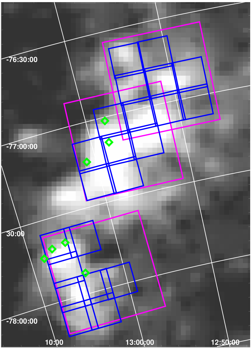
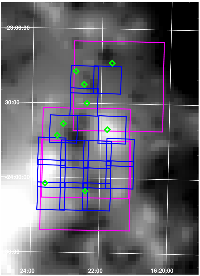
Figure 1: The locations of our survey areas in Chamaeleon II (left) and Ophiuchus (right) superposed on extinction maps from Cambrésy (1999). The magenta boxes show the positions of our MOSAIC II (I band) fields, and the blue boxes show the locations of our ISPI (near-IR) fields. The green diamonds show the locations of sources #1 to #16 in our sample of objects showing mid-IR excess emission. While observing, we dithered ISPI by up to 45″, increasing the size of our ISPI fields in some cases, as evidenced by the 2 green diamonds that fall outside of the displayed ISPI field boundaries. The A_V’s shown in the maps range from 0.1 to 5.4 in our ISPI surveyed regions of Chamaeleon II and 1.3 to 7.3 in our ISPI surveyed areas of Ophiuchus.

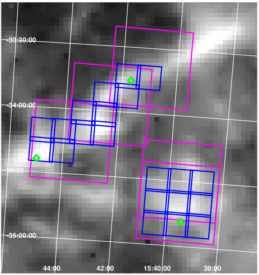
Figure 2: The locations of our survey areas in Lupus I superposed on an extinction map from Cambrésy (1999). The magenta boxes show the positions of our MOSAIC II (I band) fields, and the blue boxes show the locations of our ISPI (near-IR) fields. The green diamonds show the locations of sources #17 to #19 in our sample of objects showing mid-IR excess emission. The A_V’s shown in the map range from 1.2 to 4.8 in our ISPI surveyed regions.

The c2d program has imaged 16 square degrees toward 5 galactic star forming regions using both IRAC and MIPS. For our follow-up survey in I, J, H, and Ks, we chose areas of the c2d survey in the Ophiuchus, Chamaeleon II, and Lupus I clouds having modest extinction as shown in Figure 1 (A${}_{V}<7.5$ magnitudes; Cambrésy 1999). To select regions with evidence for recent star formation, we deliberately chose areas containing or close to concentrations of T Tauri stars known from H$\alpha$ surveys (Wilking et al. 1987; Hartigan 1993; Schwartz 1977). The positions of our fields in the Ophiuchus, Chamaeleon II, and Lupus I molecular clouds are shown in Figures 1 and 2. The total area covered and average limiting magnitudes of our survey are shown in Table 1.

2.2 Near-Infrared Imaging

We obtained J, H, and Ks images using the Infrared Sideport Imager (ISPI; van der Bliek et al. 2004; Probst et al. 2003) on the CTIO Blanco 4m telescope on 2003 May 16 & 17 and 2004 May 1–5. The 2048 $\times$ 2048 Hawaii II InSb array in ISPI has a 0.305″ pixel^-1 plate scale. K-band FWHM seeing measurements ranged from 0.6″ to 2.0″. Typical on-source integration times were 10 minutes in each band (1 minute integrations taken in a 10-point random dither pattern with maximum shifts of 45″). On-source integration times were varied with seeing to maintain uniform sensitivity limits (Table 1). The total integration time in any one band varied from 5 to 30 minutes. After flat fielding the raw frames, we masked out saturated pixels, subtracted the median from each frame, and created a sky frame by median combining the images in a 10 point dither. After subtracting the sky from each frame, we used IRAF and the IMCOADD task (part of the GEMTOOLS package) to derive the position shifts between frames and create an averaged, cosmic-ray-event cleaned image. For fields with more than 1000 matched sources with the USNO-A2 catalog (Monet 1998), we created a map of average field distortion by fitting 4th order polynomials with full cross terms in the x and y pixel directions. We combined all of the field distortion maps for each band, and applied the result to our near-IR images. After correcting for field distortion, we established the world coordinate system (WCS) for our on-source images by cross-correlating our images with the USNO-A2 catalog. Typical residuals for our WCS fit are 0.2″. We found sources in our fields using the Source Extractor package (Bertin & Arnouts 1996). We then performed aperture photometry using the PHOT task (part of the IRAF APPHOT package) with an aperture radius of 1.1 times the median FWHM of objects found in the image. The 1 $\sigma$ uncertainty for our aperture photometry was calculated by the PHOT task. ISPI uses J, H, and Ks filters from the Mauna Kea Observatory (MKO) filter set (Simons & Tokunaga 2002). To set the zero point for our photometry, we matched sources found in our survey to sources that are at least 20$\sigma$ detections in the 2MASS catalog. We transformed the matched 2MASS source magnitudes to the MKO system using the transformation equations found in the 2MASS Explanatory Supplement. For an object with a J-Ks color of 1.0 magnitude and a J-H color of 0.5 magnitudes, the uncertainties associated with the filter transformations were 0.011, 0.010 and 0.007 magnitudes in J, H, and Ks. The RMS scatter about the zero point of our sources from the zero point solution determined from the 2MASS catalog varied from 0.007 magnitudes in the best matched fields to 0.02 magnitudes in the worst matched fields. The 2MASS explanatory supplement claims calibration uncertainties of 0.011, 0.007, and 0.007 magnitudes in J, H, and Ks respectively. Therefore, we assign a conservative 0.03 magnitude calibration error to our near-infrared colors. To ensure that our catalog includes accurate near-IR photometry of objects saturated in our ISPI images, we combined our near-infrared catalog and any 2MASS sources in our fields, after transforming the 2MASS magnitudes to the MKO filter system.

2.3 Optical Imaging

We obtained our I band images using the MOSAIC II imager (Muller et al. 1998) on the Blanco 4m telescope at CTIO on 2004 March 26 & 27. The I band filter used on MOSAIC II is centered at 0.805 $\mu$m and has a FWHM of 0.150 $\mu$m. The positions of the 36′ $\times$ 36′ fields are shown in Figure 1. The plate scale of the eight 2048 $\times$ 4096 SITe CCDs is 0.27″ pixel^-1. I-band FWHM seeing measurements were $\sim$0.7″ on the night of 2004 March 26 and $\sim$1.3″ on 2004 March 27. During our observing run, one of MOSAIC II’s CCDs was inoperable. By carefully selecting our dither pattern and field placement, we made sure that all of our fields observed by ISPI were evenly covered. On the night of 2004 March 26, we took 300 s exposures over a 5 point dither pattern for 1500 s of on source integration time. Since the seeing was worse on the night of 2004 March 27, we took 300 s exposures over a 10 point dither pattern for 3000 s of on source integration time, in order to obtain roughly uniform sensitivity for data taken either night. We also took individual 30 s exposures of each field in order to achieve higher dynamic range in our catalog. The 10$\sigma$ limits for our I-band data are shown in Table 1. We used the MSCRED package in IRAF to flat-field the images, create bad pixel masks, derive the WCS for each frame, create a single images from the mosaic, and combine the images into a final averaged image, as outlined by Valdes (1997). We used Source Extractor (Bertin & Arnouts 1996) to find sources in our fields. MOSAIC II’s large field of view means that the FWHM of the PSF can vary by as much as 20% across the field. Because of this variation, we used larger aperture radii than the 1.1 times the FWHM used for our near-IR data reduction. We obtained aperture photometry using APPHOT for an aperture radius of 1.25″ with inner and outer sky radii of 5.0″ and 10.0″ respectively for data taken on 2004 March 26, and an aperture radius of 1.50″ with inner and outer sky radii of 6.0″ and 12.0″ respectively for data taken on 2004 March 27. Photometric zero points were obtained by observing Landolt standard fields (Landolt 1992) and adding a linear term to correct for airmass as well as an offset for the aperture correction. The RMS scatter about the zero point correction was 0.007 magnitudes for standard fields observed on 2004 March 26 and 0.006 magnitudes for fields observed on 2004 March 27. Comparing data taken in overlapping fields, we found that our positions agreed to better than 0.25″ while our magnitudes agreed to better than 0.05 magnitudes. We therefore assign a positional uncertainty of 0.25″ and a photometric error of 0.05 magnitudes to our I band photometry.

2.4 C2D Observations

As part of the c2d Legacy Project (Evans et al. 2003), Spitzer has mapped 8.0 square degrees of the Ophiuchus molecular cloud, 1.1 square degrees of the Chamaeleon II molecular cloud and 2.4 square degrees of the Lupus molecular clouds with IRAC (3.6, 4.5, 5.8, and 8.0 $\mu$m; Fazio et al. 2004) and MIPS (24 $\mu$m; Rieke et al. 2004). The IRAC maps consist of two epochs, separated by several hours, each with two dithers of 12 s observations (48 s total). The second epoch observations were taken in the High Dynamic Range mode which include 0.6 s observations before the 12 s exposures, allowing photometry of both bright and faint stars. MIPS observations were taken in the fast scan mode, also in two different epochs of 15 s exposures each. The average 10 $\sigma$ sensitivities of the c2d survey of molecular clouds are shown in Table 1. Detailed descriptions of the MIPS and IRAC observing procedures used by c2d can be found in Young et al. (2005) and Harvey et al. (2006).

2.5 IRAC and MIPS Photometry

We searched preliminary c2d IRAC and MIPS point source catalogs for fluxes of brown dwarf candidates selected in the near-IR (see §3.1), and used these fluxes when available. The c2d catalogs were produced using the c2d mosaicking/source extraction software, c2dphot (Harvey et al. 2006), which is based on the mosaicking program APEX developed by the Spitzer Science Center and the source extractor Dophot (Schechter et al. 1993). Since the preliminary c2d catalogs in the archive are complete down to only $\sim$ 20 $\sigma$ detections (see Evans et al. (2005) for a detailed description of the c2d data products), we had to extract our own fluxes from the c2d images for many of our sources (especially at 5.8 and 8.0 $\mu$m). To ensure consistency, we extracted fluxes not present in the c2d catalogs using the c2dphot software in a mode that allows us to obtain fluxes (and upper limits) of low S/N sources with known positions. In this mode, c2dphot calculates the fluxes by fitting a PSF to fixed positions. The only free parameters are the background level and peak intensity. The flux uncertainty is calculated from the goodness of the fit. The input coordinates were taken from our near-IR observations which, in general, show a coordinate agreement of $\lesssim$ 0.3″ with c2d sources. We consider $\geq$ 5 $\sigma$ detections to be real. For all detections, however, we examine the images using the IRAF IMEXAMINE task, and make sure the object is a point-source and well detected above the background. We note that the error in the photometry of high S/N sources is dominated by the absolute calibration uncertainty for the c2d IRAC and MIPS catalogs ($\sim$15$\%$; Evans et al. 2005).

3 Results

3.1 Source Selection

In our Chamaeleon II, Ophiuchus, and Lupus I fields, we detected $\sim$120,000 sources at 5 $\sigma$ or better in the I-band and all three near-IR bands. From our full catalog, we wish to select only objects that 1) are likely young stellar objects and 2) show evidence of mid-IR excess emission from circumstellar material. To create our final list of young sources with mid-IR excess emission, we must weed out extragalactic objects, background stars, and foreground stars.

Even in the presence of foreground reddening, extragalactic objects have near-IR colors that allow them to be distinguished from brown dwarfs. The Munich Near-Infrared Cluster Survey (Drory et al. 2001) covers $\sim$1 square degree at high galactic latitudes to limiting I, J, and K magnitudes of 22.4, 21.0 and 19.5 respectively. Galaxies from Drory et al. (2001) typically have I-J colors of $\sim$1.0. For young M-type objects, later spectral types, and hence lower effective temperatures correspond to redder intrinsic I-J colors (Briceño et al. 2002; Luhman 2004). The trend of redder I-J colors with later spectral type is also observed for M, L and T spectral type field brown dwarfs (Dahn et al. 2002). The average I-J color of young M6 objects (Briceño et al. 2002; Luhman 2004) is 2.42. The number counts of galaxies increase as one moves to fainter magnitude bins (Drory et al. 2001). Thus, we require strict selection criteria (redder I-J colors) for faint objects, and loosen our selection criteria for brighter objects.

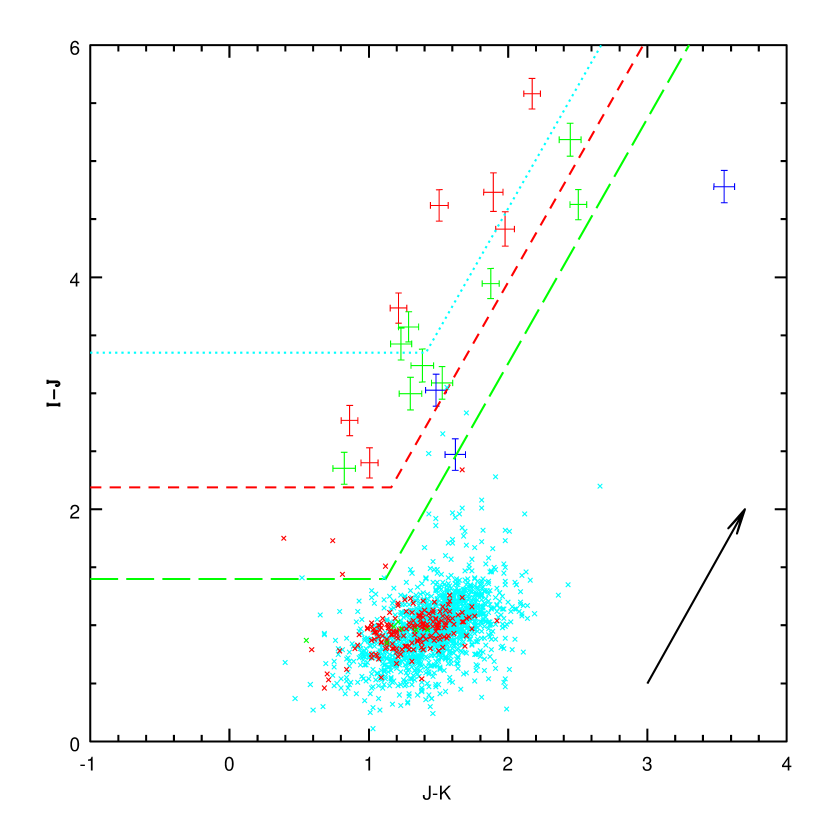
Figure 4: Our color-color source selection criteria. The points with error bars are objects #1 to #16 in Table 3. The X’s show galaxies from Drory et al. (2001). The cyan sources have K magnitudes less than 9.81 + the distance modulus to Chamaeleon II ($\mu_{d}=$ 6.25). These sources must lie above the cyan dotted line to meet our selection criteria. Similarly, to meet our selection criteria, the red sources (K magnitudes between 9.81 and 6.94 + $\mu_{d}$) must lie above the red dashed line and the cyan sources (K magnitudes between 6.94 and 4.49 + $\mu_{d}$) must lie above the cyan long-dashed line. The blue sources have K magnitudes brighter than 4.49 + $\mu_{d}$ and have no color criteria for selection.

We initially cut our sample based on the I, J, H, Ks colors and magnitudes of the objects. We start with 120,000 sources detected at $>5~{}\sigma$ in I, J, H, and Ks, and apply different selection criteria depending on whether the object’s K magnitude is fainter than expected for a young M9 object, between the expected K magnitudes for young M6 and young M9 objects, between the expected K magnitudes for young M3 and young M6 objects, or brighter than the K magnitudes of young M3 objects. We determine the colors and magnitudes of young M objects from samples in Taurus and Chamaeleon I (Briceño et al. 2002; Luhman 2004). Our near-IR source selection criteria are illustrated in Figures 3 and 4. The average absolute K magnitude of young M8.5 to M9.5 objects in Taurus and Chamaeleon I is 8.01 (Briceño et al. 2002; Luhman et al. 2004). The bluest I-J color of a young M8.5 to M9.5 object with an absolute K magnitude less than 8.01 is 3.35. Thus, for objects with observed K magnitudes fainter than 8.01 plus the distance modulus to the cloud, $\mu_{d}$ (Table 2) we select only objects with I-J$>$3.35. To ensure that we do not add reddened galaxies to our sample, we deredden the objects to the average J-K color (1.41) of M8.5 to M9.5 young brown dwarfs, and select objects with a dereddened I-J$>$3.35 (including photometric errors). We use A_λ/A_V values for our I, J, and Ks filters (0.56, 0.26, and 0.12 respectively) from the Asiago Database on Photometric Systems (Fiorucci & Munari 2003). For objects which range in magnitude between the average absolute K magnitude for young M8.5 to M9.5 dwarfs reddened by A_V=15 and the average absolute K magnitude of young M6 objects (9.81 and 5.14 respectively) + $\mu_{d}$, we require I-J$>$2.19 when dereddened to a J-K of 1.16 (appropriate for young M6 objects). For objects with K magnitudes between the average of young M6 objects reddened by A_V=15 and the average absolute K magnitude of young M3 stars (6.94 and 2.69 respectively) + $\mu_{d}$, we require I-J$>$1.40 when dereddened to a J-K of 1.12 (appropriate for young M3 objects). Objects brighter than the intrinsic K magnitude of young M3 objects + $\mu_{d}$ are few in number (63), and none of the galaxies from Drory et al. (2001) are this bright, so we include all of these sources in our initial sample. For each object meeting our color and magnitude selection criteria, we examine the object’s PSF to ensure that is a point source. 5853 objects toward Ophiuchus, 1504 objects toward Chamaeleon II, and 4977 objects toward Lupus I meet our initial selection criteria. None of the $\sim$3300 galaxies observed by Drory et al. (2001) that are within the detection limits of our near-IR survey (Table 1) meet our near-IR selection criteria for young brown dwarfs, even if we redden the galaxies by A_V=5. We also compared templates of all the galaxy types fit to objects in the Lockman hole (Polletta et al., in preparation) by red shifting them from z=1 to 4 and reddening them from A_V=0 to 10. None of the Polletta et al. model templates which might appear as point sources in our I-band images meet our selection criteria.

For the sources meeting our near-IR selection criteria, we make an additional cut by looking for mid-IR excesses. At the galactic latitudes of the clouds in our survey (b $\sim$ 18, 16 and -14 for Ophiuchus, Lupus I, and Chamaeleon II respectively), there are no known star-forming regions behind our clouds. By looking for objects with evidence of emission in the mid-IR significantly in excess of the photospheric emission extrapolated from the near-IR colors (i.e., evidence for a disk or circumstellar material), we will ensure the young age (and hence cloud membership) of candidates in our sample, effectively eliminating any field-population background or foreground stars or brown dwarfs, which will not have excess emission. We obtain mid-IR fluxes for the 12334 objects meeting our near-IR selection criteria using the method described in §2.5. Using the near-IR colors of objects in our sample, we fit reddening simultaneously with the observed I, J, H and Ks colors of young M-type objects in Chamaeleon I and Taurus (Briceño et al. 2002; Luhman 2004) as described in §3.2. To estimate the expected mid-IR emission from the photosphere of our best fit young object, we use the observed IRAC colors of field brown dwarfs (Patten et al. 2004). If an excess exists at [5.8] and [8.0] of greater than 3 $\sigma$ above the best fit young M-type object colors, we examine the near and mid-IR images to make sure that the object is a point source, since IRAC bands 3 and 4 suffer from substantial nebulosity. Table 3 contains the observed I, J, H, Ks, and IRAC magnitudes for the 19 sources in our survey that have colors and magnitudes meeting our selection criteria and which appear as point sources in the I, J, H, Ks and IRAC images. Sources #1–#19 are detected in all of the IRAC bands as well as in MIPS1, with excess emission above that expected from the photosphere in IRAC3, IRAC4, and MIPS1. Flux densities from 3.6 to 24 $\mu$m for objects #1 to #19 are shown in Table 4. The SEDs of 18 of the sources comprising our sample are shown in Figures 5 and 6, where the open circles show the observed data and the filled circles show the extinction-corrected data; we omitted source #3, the brightest object in our sample.

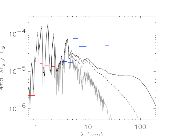
Figure 7: Theoretical SED of a 1 Myr old, 2 M_J sub-brown dwarf at the distance to Ophiuchus (125 pc; de Geus et al. 1989)). The grey line shows the theoretical photospheric emission of a 1 Myr old, 2 M_J object (1300 K, log(g)=3.5; Baraffe et al. 2003; Allard et al. 2001). Theoretical SEDs for a 2 M_J object with a flared (solid line) and a flat (dashed line) circumstellar disk are also shown (See §5 for details of the disk models). We chose parameters for our disk models ($i=$ 0^∘, and $R_{i}=R_{\ast}$) that produce the largest mid-IR fluxes. The horizontal lines denote the band widths and 10 $\sigma$ sensitivity limits of our I, J, H, and Ks survey toward Ophiuchus along with 10 $\sigma$ IRAC and MIPS 1 sensitivity limits of the c2d survey toward Ophiuchus. Though a 1 Myr old, 2 M_J sub-brown dwarf would be easily detected by our near-IR survey, it is below the c2d sensitivity limits in IRAC 3, IRAC 4, and MIPS 1, even with excess emission from a flared disk.

None of the 19 sources in our sample have K magnitudes that fall in our faintest magnitude bin (8.01 plus A_V=15 + $\mu_{d}$) for selection criteria. The faintest observed K magnitude of our sample is 3 magnitudes brighter than our 10 $\sigma$ limit. The c2d survey does not have the sensitivity in IRAC bands 3 and 4 to detect objects with fainter intrinsic K magnitudes. Figure 7 shows the theoretical SED for a 1 Myr old, 2 M_J sub-brown dwarf (Baraffe et al. 2003; Allard et al. 2001) along with models of two possible circumstellar disks (§ 5 details our disk modeling procedure). Even though this object would be detected easily in our near-infrared survey, it is fainter from 5.8 to 24 $\mu$m than the 10 $\sigma$ c2d IRAC and MIPS limits. 1633 sources in our survey have 0.8 to 4.5 $\mu$m colors which meet the selection criteria for objects fainter than M9, but are not detected in IRAC3, IRAC4 and MIPS1. Some of these objects may be very low-mass objects with disks.

We have tested our source selection in several ways. Examination of the colors of young brown dwarfs with disks shows that we can recover objects of this type. Natta et al. (2002) successfully fit excess emission (as detected with ISOCAM) around young brown dwarfs in the core of Ophiuchus with models of emission from a circumstellar disk. More recently, Luhman et al. (2005b, c) detected (with IRAC) and modeled circumstellar disks around two brown dwarfs in Chamaeleon I (Cha 1109-7734 and OTS44) with masses of $\sim$8 and $\sim$15 M_J. Using I-band fluxes from the the literature, 2MASS or published near-IR magnitudes (transformed to the MKO system), and IRAC fluxes from c2d (Allen et al. 2006, in preparation) or Luhman et al. (2005b, c), we have applied our near-IR selection criteria to these 8 objects and then searched for mid-IR excesses as outlined above. Cha 1109-7734, OTS44, and all of the Natta et al. (2002) objects meet our selection criteria. Six of the more luminous sources among the 19 in our sample have been identified in other surveys searching for young stars and brown dwarfs, which also lends credibility to our selection criteria. Sources #2 and #3 were identified as young objects using DENIS J and Ks and ISOCAM 6.7$\mu$m and 14.3$\mu$m photometry (Persi et al. 2003). Source #3 was also detected in soft (0.1–0.5 keV) and hard (0.5–2.5 keV) X-ray emission with ROSAT (Alcalá et al. 2000). Sources #4, #6, & #7 were identified as low-mass T Tauri or young brown dwarf candidates by Vuong et al. (2001). Based on their strong H$\alpha$ emission, sources #4 and #10 have previously been identified as the T Tauri stars Sz52 and WSB 14 respectively (Schwartz 1977; Wilking et al. 1987). Finally, follow-up near-IR spectra of 5 of our sources in Table 3 (#1, #2, #5, #11, & #14) have confirmed their identification as young brown dwarfs (Allers et al. in preparation).

3.2 Estimating Extinctions and Luminosities

To determine the extinction toward our sources, we deredden and fit them to the observed colors of young M-type objects in the Taurus and Chamaeleon I star forming regions (Briceño et al. 2002; Luhman 2004). We deredden our colors based on A_λ/A_V values of the MKO filter and Bessell filter systems in the Asiago Database on Photometric Systems (Fiorucci & Munari 2003), for the R_V=3.1 extinction law of Fitzpatrick (1999). For IRAC and MIPS wavelengths, we use the values of A_λ/A_V for the R_V=3.1 extinction law of Fitzpatrick (1999) averaged over the filter bandpasses. The values of A_λ/A_V used are 0.56, 0.26, 0.17, 0.12, 0.06, 0.04, 0.03, 0.02, and 0.0 for I, J, H, Ks, [3.6], [4.5], [5.8], [8.0], and [24] respectively. The R_V=5.0 extinction law provides the same A_λ/A_V for near and mid-IR bands, and only slightly changes A_λ/A_V for the I band (to 0.60). Since near-IR colors get redder as one moves to later spectral types, several of our objects can be fit to either a late spectral type object with low extinction or an earlier type object attenuated by more dust. To break this degeneracy, we can limit the range of spectral types that we use to fit our objects based on the K magnitudes of our sources. Objects with absolute K magnitudes brighter than expected for a young M6 objects (5.14; §3.1) are fit to the colors of young objects with spectral types from M3 to M8, while objects with absolute K magnitudes fainter than expected for young M9 objects (8.01) are fit to the colors of young M6 to M9.5 objects. Objects between these extremes are fit to the colors of young M3 to M9.5 objects. Even these fairly loose restrictions are sufficient to leave only one dereddening solution for each object. Table 5 shows the calculated A_V for each of our sources. When we use this technique to derive A_V for the Chamaeleon I objects Cha 1109-7734 and OTS44 (Luhman et al. 2005b, c), our calculated extinctions (A_V=2 magnitudes for both sources) agree to within the uncertainties with the published extinctions (A_V = 1 $\pm$ 1 mags). We also calculated A_V’s for six brown dwarfs with disks from Natta et al. (2002). Our calculated A_V’s are on average 0.3 magnitudes higher than the published A_V’s in Natta et al. (2002), which have an uncertainty of $\pm$1 mag; the largest variations were A_V=2 mags. We assign an uncertainty in A_V of $\pm 2$ mags for our calculated extinction values.

We calculate the stellar luminosity by integrating the dereddened flux density from I through [3.6] over the frequency width of the filters. For wavelengths between bandpasses, we linearly interpolated the flux densities and integrated them over the frequency gap between the bands. We calculate the bolometric luminosity based on the sum of the flux in and between the bands, assuming the distances in Table 2. As a check, we applied our method for calculating bolometric luminosities to field brown dwarfs from Golimowski et al. (2004) using [3.6] fluxes from Patten et al. (2004). We find that our calculated luminosities typically agree with the Golimowski et al. (2004) values to better than 5%. Excess emission at [3.6] does not greatly affect our luminosity calculations. Liu et al. (2003) detected L^′ excesses around late-M-type young brown dwarfs. Including the largest K-L^′ excess (0.45 magnitudes) from Liu et al. (2003) in the [3.6] magnitude of the field dwarfs from Patten et al. (2004) increases the calculated luminosity by at most 7% relative to the same source with no excess. The uncertainties in cloud distance (Table 2) correspond to uncertainties of 0.09, 0.12, and 0.18 dex in Chamaeleon II, Lupus I, and Ophiuchus respectively. The luminosity uncertainties resulting from uncertainties in distance, A_V (0.15 dex), and our method of calculating the luminosity (0.02 dex) combine for a total uncertainty of $\pm$0.24 in log L_∗ for our Ophiuchus sources, $\pm$0.19 in log L_∗ for our Lupus I sources, and $\pm$0.18 in log L_∗ for sources in Chamaeleon II. Our sources have luminosities ranging from 0.5 $>$ log(L_∗/L_⊙) $>$ -3.1 (Table 5). The mean log(L_∗/L_⊙) of our sample is $-1.8$. Four of the objects in our sample (#1, #5, #12, & #17) have luminosities that are equivalent (to within the uncertainties) to the lowest luminosity young brown dwarf with mid-IR excess reported to date (Luhman et al. 2005b).

3.3 Ages

The ages of objects in our sample are relevant because we assume an age and use a theoretical isochrone for that age to estimate the mass and T_eff of our objects using their luminosities. The ages of stars in the clouds in our survey have been determined mainly from the ages of T Tauri stars and brown dwarfs with masses greater than 20 M_J. Placing young objects on the H-R diagram in order to determine their ages is difficult. The distances to the sources are usually assumed to be similar to the distance to the parent cloud (which in itself is usually only accurate to $\pm$ 10 pc). The stellar luminosity is usually found by estimating the reddening and using a bolometric correction to a single dereddened band (usually I or J bands). In addition, T_eff is usually determined from a SpT-T_eff relationship, and not determined empirically. The age determinations in the literature depend strongly on the evolutionary models overlaid on the H-R diagram. For example, the models of D’Antona & Mazzitelli (1994) yield ages that are a factor of $\sim$3 lower than Baraffe et al. (2003) age estimates (e.g. Cieza et al. 2005). The combination of these uncertainties makes estimates of ages for individual sources very uncertain. The definition of age itself differs from model to model. Some models arbitrarily take the zero age to be the point when a contracting, fully convective object starts to move down the Hayashi track (e.g. D’Antona & Mazzitelli 1994; Baraffe et al. 1998), whereas other models define the birthline based on the conditions of the star at the onset of deuterium burning (Palla & Stahler 1999). Whether or not the same age can be applied to stars, brown dwarfs, and objects with masses below the deuterium burning limit remains unclear. In addition, the models do not include the effects of accretion through a disk. Since we do not have spectral types for our objects, we must estimate their effective temperatures and masses from model isochrones (Baraffe et al. 2003) by assigning an age based on values found in the literature. Fortunately, uncertainties in age of $\pm$2 Myr (for objects with estimated ages of 3 Myr) correspond to uncertainties in effective temperature of less than 100 K according to the isochrones of Baraffe et al. (2003). Mass uncertainties resulting from mis-estimation of ages are slightly larger. The lowest luminosity sources in our survey (log($L_{\ast}/L_{\odot})\sim-3.0$) correspond to masses of $\sim$6 M_J for the 1 Myr isochrone, and correspond to masses of $\sim$15 M_J for the 5 Myr isochrone.

3.3.1 Ophiuchus

Luhman & Rieke (1999) find a median age of 0.3 Myr for the objects in the core of Ophiuchus using luminosities estimated from J band fluxes and the isochrones of D’Antona & Mazzitelli (1994), in agreement with previous work (Greene & Meyer 1995). Prato et al. (2003) find ages ranging from 0.4 to 1.5 Myr for several young binaries in the Ophiuchus region by estimating stellar luminosities as the luminosity of blackbody at the T_eff of the star scaled to fit the observed J and H band fluxes and deriving an age from the isochrones of Palla & Stahler (1999). More recently, Wilking et al. (2005) find a median age of 2.1 Myr for sources surrounding the Ophiuchus cloud core. Given the young age that most authors find for Ophiuchus, we adopt an age of 1 Myr for our sources in Ophiuchus, which is the youngest isochrone of the Baraffe et al. (2003) models.

3.3.2 Chamaeleon II

Alcala et al. (1997) find a mean age of 1.3 Myr for T Tauri stars in Chamaeleon II, based on stellar luminosities derived from measured I band fluxes and the evolutionary tracks of D’Antona & Mazzitelli (1994), in agreement with earlier work Hughes & Hartigan (1992). Recently, Cieza et al. (2005) find an average age of 3.6 Myr for classical T Tauri stars in Chamaeleon by placing objects on the HR diagram along with the evolutionary tracks of Baraffe et al. (1998) based on luminosities derived from the I band flux, and temperatures based on the spectral type of the objects. Since we are using the Baraffe et al. (2003) isochrones in subsequent sections of this paper, and published isochrones are available at young ages of 1, 3, 5, and 10 Myr, we adopt an age of 3 Myr for our sources in Chamaeleon II.

3.3.3 Lupus I

Wichmann et al. (1997) find a mean age 1.2 Myr for classical T Tauri stars in the Lupus star forming region, and a slightly older mean age of 3.1 Myr for weak line T Tauri stars by calculating stellar luminosities from blackbody fits to the R band (with T_eff given from the spectral type of the object), and getting ages of the stars from the evolutionary tracks of D’Antona & Mazzitelli (1994). This is in agreement with Hughes et al. (1994), who find that Lupus I and II contain a younger stellar population than Lupus III or IV, and estimate an age of $\sim$1 Myr for classical T Tauri stars in Lupus I and II. For Lupus I, we adopt an age of 1 Myr.

4 Analysis

4.1 Masses

Using ages of 1 Myr for Ophiuchus and Lupus I and 3 Myr for Chamaeleon II, we estimate the effective temperatures and masses of our 19 objects by matching the source luminosities to the isochrones of Baraffe et al. (2003) and Baraffe et al. (1998). Our sample includes five sources with nominal masses below the deuterium burning limit, the lowest luminosity source in our sample (log(L_∗/L_⊙)$=-3.1$) having a mass possibly as low as 6 M_J. Sources in the Trapezium cluster having similar dereddened absolute H-band magnitudes to the faintest sources in our sample also have similar mass estimates (8–11 M_J; Lucas et al. 2001). Our mass estimates rely heavily on the assumed ages for our sources. If our sources are actually 10 Myr old, the inferred mass of a log(L_∗/L_⊙) = -3.1 source would be 15 M_J. Additional uncertainty in the nominal masses of our sources originates in the evolutionary models themselves. Hillenbrand & White (2004) find that the evolutionary models underpredict the dynamically determined masses of pre-main sequence stars by as much as 30%. For young brown dwarfs, no dynamical mass constraints are available in the current literature. Thus the evolutionary models are relatively untested in the young, low-mass regime, and masses determined from the models are highly uncertain (Baraffe et al. 2002).

4.2 Accretion vs. Reprocessing Luminosities

If the mid-IR excess emission we observe can be attributed to a circumstellar disk, what is the heating mechanism for the disk? For a flat, optically thick disk extending outward from the stellar surface, the luminosity due to reprocessing of light from the irradiated disk is

$$L_{irrad}=0.25L_{\ast},$$ (1)

where L_∗ is the source luminosity. The maximum luminosity generated by viscous dissipation of accretion within the disk is

$$L_{acc}=\frac{GM_{\ast}\dot{M}}{2R_{\ast}},$$ (2)

where M_∗ and R_∗ are the mass and radius of the central object, and $\dot{M}$ is the accretion rate for material moving onto the central object from the disk.

Modeling H$\alpha$ emission, Muzerolle et al. (2005) find low accretion rates for brown dwarfs in Taurus and Chamaeleon I with masses of 25 M_J ($\dot{M}$ $\sim$ 5 $\times$ 10^-12 M_⊙ yr^-1). For objects of 25 M_J on the 1 Myr isochrone, Baraffe et al. (2003) predict R_∗ $\simeq$ 0.40 R_⊙, log(L_∗/L_⊙) $\simeq$ -2.2. Using these values along with the equations above, we calculate L_irrad/L_acc $\sim$320. The mass accretion rate depends strongly on the stellar mass, with $\dot{M}$ $\propto$ M^2.1 for observations down to 25 M_J (Muzerolle et al. 2005). If this relationship holds to lower masses, we would expect a 10 M_J object to have $\dot{M}$ $\sim$ 7 $\times$ 10^-13 M_⊙ yr^-1. The Baraffe et al. (2003) models predict R_∗ $\simeq$ 0.30 R_⊙ and log(L_∗/L_⊙) $\simeq$ -2.7 for a 1 Myr old, 10 M_J object leading to a ratio of radiative luminosity to luminosity from viscous dissipation of accretion, L_irrad/L_acc $\approx$1200. Due to the smaller gravitational force experienced by their disks, brown dwarf disks should be highly flared, with scale heights up to 3 times those found for classical T Tauri stars (Walker et al. 2004). In addition, if the disks have inner holes, then the inner radius of the disk would be the relevant radius in equation 2. Best-fit models of the excess emission around two low mass brown dwarfs, OTS44 (Luhman et al. 2005c) and GY11 (Natta & Testi 2001), indicate that low mass brown dwarfs can have inner radii of 3 R_∗. Thus, our estimate of L_irrad/L_acc is likely a lower limit. The observational evidence to date suggests that accretion should not play a major role in the heating of circumstellar material around low mass brown dwarfs.

4.3 Excess vs. Stellar Luminosities

The availability of fluxes over a broad range of near and mid-IR wavelengths for all the objects in our sample permits us to compare stellar and excess luminosities without the usual uncertainties introduced by using bolometric corrections to estimate the stellar luminosity or by measuring the excess at wavelengths where the object’s photosphere dominates the emission. The upper panel of Figure 8 shows the ratio of the 5.8 through 24 $\mu$m excess luminosity to the stellar (or central object) luminosity versus stellar luminosity, along with linear fits to all of our data points (dotted line) and excluding sources #12 and #3 (dashed line). The ratio of excess to stellar luminosities is remarkably constant across three orders of magnitude in stellar luminosity. A linear fit (ordinary least-squares regression) to the data excluding sources #12 and #3 (two obvious outliers) shows that the ratio of excess to stellar luminosity scales as L^-a, where $a=0.04\pm 0.04$. The mean 5.8–24 $\mu$m excess to stellar luminosity ratio for our sample (excluding sources #12 and #3) is 0.12 $\pm$ 30%. The mean 5.8–24 $\mu$m excess to stellar luminosity ratio is lower than the minimum reprocessing luminosity (Equation 1), because we are not including flux longward of 24 $\mu$m, where much of the energy from the disk is emitted. In the lower panel of Figure 8, we try to determine if the roughly constant ratio of excess to stellar luminosity holds for other samples of young, low-mass objects. Since a consistent data set of the disk luminosity is not available for other very low luminosity brown dwarfs, we plot the ratio of excess 8.0 $\mu$m luminosity to the photospheric luminosity and include results for the Natta et al. (2002) and Luhman et al. (2005b, c) brown dwarfs with disks. Most of these additional sources are consistent with the constant ratio of excess to stellar luminosities that we find for higher luminosity sources. The results for OTS44 (Luhman et al. 2005c) and the 2 lowest luminosity sources from Natta et al. (2002) show enhanced excess flux at 8 $\mu$m, consistent with a possible trend toward higher ratios of excess to stellar luminosity for very low luminosity brown dwarfs. The constant ratio of excess to stellar luminosity for our sources is remarkable. It implies that, whatever the details of the disk structure may be, the inner disks of young stars, brown dwarfs and sub-brown dwarfs intercept and reprocess about the same fraction of radiation from the central object.

5 Modeling the SEDs

In Figures 5–6, we show the SEDs of 18 of the 19 sources in our sample with detections in all bands (I to MIPS1). Source $\#$3 is not modeled as the luminosity of this source lies outside of the range covered by the Baraffe et al. (1998) models. If we match the source luminosities to the 1 Myr (for Ophiuchus and Lupus I) and 3 Myr (for Chameleon II) isochrones of Baraffe et al. (2003) or Baraffe et al. (1998), then Figure 5 includes sources with inferred masses of 6–50 $M_{J}$ ($\rm{log}(L_{\ast}/L_{\odot}){\leq}-1.8$). and Figure 6 includes sources with masses of 50–350 $M_{J}$ ($\rm{log}(L_{\ast}/L_{\odot}){\geq}-0.7$).

Table 6 lists the luminosity, effective temperature, mass, radius and gravity of the evolutionary model (Baraffe et al. 2003, 1998) with L_model closest to L_source at the age of the cloud (Table 2). The stellar atmosphere models (Allard et al. 2001; Hauschildt et al. 1999, grey lines in Figures 5 and 6) are for the T_eff listed in Table 6 rounded to the nearest 50 K, and a gravity, log($g$) = 3.5, appropriate for 1–3 Myr objects. For objects near or above the stellar limit (i.e., for $T_{eff}\geq 3000$ K), we use the PHOENIX model atmospheres for low mass stars (Hauschildt et al. 1999). For substellar objects ($T_{eff}\leq$ 3000 K), we use AMES-dusty models, which include dust formation in the chemical equilibrium calculations and the contribution of dust opacities to the total optical depth. The atmospheric models shown in Figure 5–6 have not been scaled to fit the data, but are simply multiplied by a dilution factor $f=(R_{\ast}/d)^{2}$, using the distances from Table 2. The coincidence between the atmospheric models and the flux in the 0.9–3.6 $\mu$m range is generally quite good, with clear excesses visible beyond 5.0 $\mu$m. The model atmospheres generally predict bluer near-IR colors than are observed.

In order to interpret the observed excesses, we compare the observed SEDs to model predictions for passive, irradiated disks (CGPLUS; Dullemond et al. 2001). CGPLUS is based on the Chiang & Goldreich (1997, hereafter CG97) model of a flared two-layer disk. The CG97 model assumes vertical hydrostatic equilibrium, resulting in a flared structure. In this model, the dust and gas are well mixed and no dust settling has occurred. The optically thin disk surface layer is irradiated directly by the central object. Superheated dust grains in the surface layer re-radiate into the disk interior and thus regulate the interior disk temperature. CGPLUS is a modified version of CG97, including the addition of a puffed up inner disk wall, the height of which is calculated self-consistently. Although CGPLUS has not previously been applied to brown dwarfs, similar models have proven to be adequate representations of disks around sub-stellar objects (Natta & Testi 2001).

For simplicity, we begin with disk model parameters very similar to those of T Tauri stars. For a source of estimated mass $M_{\ast}$, we adopt a disk mass of 0.03 ${M_{\ast}}$ and a fixed outer disk radius of 5 AU. Increasing the disk outer radius does not change the SED shortward of  25 $\mu$m, and thus our observations cannot constrain this outer radius. However, for our lowest mass objects, the disk scale heights become unreasonably large at R $\gtrsim 5$ AU, such that the material is no longer gravitationally bound to the central source. The surface density of the disk varies as $R^{-1}$ and opacities are from Laor & Draine (1993). All sources are modeled with flat and flared face-on disks ($i=0^{o}$) with a disk inner radius equal to the stellar radius ($R_{i}={R_{\ast}}$). Where necessary, additional models with larger inner disk radii and inclinations are calculated.

We test the effects of the disk inclination, disk flaring and the size of the inner disk hole on the strength/shape of the excess. In general, SEDs of flared inclined disks (e.g. $i=60^{o}$) are quite similar to SEDs of flat face-on disks for $\lambda\leq 24$ $\mu$m, and our IRAC observations often cannot distinguish between these two models. For flat inclined disks (e.g. $i=60^{o}$), the flux falls off more rapidly as a function of wavelength. If the inner radius is increased to $R_{i}>R_{\ast}$, then the flux in the IRAC bands becomes more photospheric. For flat disks with $R_{i}>R_{\ast}$, the flux beyond $\lambda\approx 15$ $\mu$m is similar to a flat disk with $R_{i}=R_{\ast}$. For flared disks with large inner holes ($R_{i}>R_{\ast}$), the flux beyond $\lambda\approx 15$ $\mu$m increases because the surface layer of the disk is warmer at larger radii.

The best fit models are overlaid in green in Figures 5 and 6 and the parameters for these models are listed in Table 6. The SEDs of all but one of the sources in this sample have power-law slopes of the SED, $a$, in the range of 1.2–2 (where ${\nu}F_{\nu}\propto{\nu}^{a}$) and can be fit well by models of flared and/or flat disks (see Figure 6). The exception is $\#$12, for which the photospheric model fits well, but the excess at $\lambda\geq 5.8$ $\mu$m is too large to be fit with the models presented here. An actively accreting disk or non-disk geometry (such as a tenuous dust envelope), might be able to explain the mid-IR excess for source #12, but a quantitative analysis of these scenarios is beyond the scope of this paper. Both flared disks with large inclinations $i\geq 60^{o}$ and face-on flat disks fit sources with $a\approx{4/3}$ (#5, #7, #11 and #16). The distinction between flared, inclined disks and flat, face-on disks relies on the accuracy of one data point, our 24$\mu$m flux measurement, and is thus the least constrained parameter of our model fits. About half of the SEDs show extremely low excesses in the 3.6–5.8 $\mu$m range and the SEDs can be fit best with a disk model possessing a larger inner radius ($R_{i}=$2–10 ${R_{\ast}}$; e.g., $\#$1 and $\#$3).

The sub-brown dwarfs in our sample to which we can fit disk models (#1, #5, #11, & #17) are fit by 3 flat disks and 1 flared disk, and a range of inner disk radii ($R_{i}=1-4R_{\ast}$). The average inner disk radius we fit to sub-brown dwarfs is $R_{i}\simeq 2R_{\ast}$. The brown dwarfs in our sample (#7, #8, #9, #13, #14, #18, and #19) have a similar distribution of flared vs. flat disks (2 out of 7 are flared) and disk inner radii (with the exception of #9, $R_{i}\simeq 2R_{\ast}$ on average) as the sub-brown dwarfs. The young stars in our sample have an average inner disk radii, $R_{i}\simeq 2R_{\ast}$, but have a larger fraction of flared disks (4 out of 6 are flared) than found for the brown dwarfs in our sample. The similarity of the disk properties for young stars, brown dwarfs and sub-brown dwarfs, along with the constant ratio of excess to stellar luminosities (§4.3), indicates that disks across the mass range probably form and evolve in similar ways.

6 Conclusions

In this paper we have presented a sample of young objects with luminosities ranging from 0.5 $>$ log(L_∗/L_⊙) $>$ -3.1 in the Chamaeleon II, Ophiuchus, and Lupus I star-forming clouds. The lowest luminosity sources in our sample (log(L_∗/L_⊙) $<$ -3.0) have inferred masses of 6–12 M_J based on the 1 and 3 Myr isochrones of Baraffe et al. (2003). The 5.8–24 $\mu$m fluxes of these objects show evidence of excess emission above the photosphere, presumably from a circumstellar disk. The ratio of 5.8–24 $\mu$m excess to stellar luminosity is constant (to within 30%) over three decades in luminosity.

Most of the near-IR fluxes of our objects agree with the predictions of stellar atmosphere models (Allard et al. 2001). Given that our choices of T_eff and log(g) are based on the measured source luminosities and model isochrone predictions of stellar luminosities at the ages of Chamaeleon II (3 Myr), Lupus I and Ophiuchus (1 Myr), rather than to fits of the spectral energy distributions, the agreement is remarkable. In general, the stellar atmosphere models tend to overestimate the I-band flux, and predict bluer near-IR colors. The origin of the discrepancy between the observations and model spectra can be explored once spectra are obtained for these objects.

Theoretical models of passive irradiated disks fit the excess emission of all but one of the objects in our sample. We find that flared, inclined disks have similar SEDs to flat, face-on disks in the IRAC wavelengths, but our observations at 24 $\mu$m can distinguish between the two in most cases. We fit a similar distribution of flared vs. flat disks, disk inclination angles, and disk inner radii to the young stars, brown dwarfs, and sub-brown dwarfs in our sample.

Table 1: Observations

Cloud	Area	10$\sigma$ Limit
		I	J	H	Ks	[3.6]	[4.5]	[5.8]	[8.0]	[24.0]
	sq. arcmin	mag								mJy
Chamaeleon II	2200	22.9	19.7	19.1	18.6	17.5	16.8	14.7	14.4	0.9
Ophiuchus	1700	23.5	20.2	19.6	18.9	17.1	16.4	14.1	13.7	0.7
Lupus I	2100	23.3	20.0	19.4	18.8	17.4	16.5	14.3	13.9	0.9

Table 2: Adopted Cloud Parameters

Cloud	distance	modulus	Age
	pc	mag	Myr
Chamaeleon II	178$\pm$18	6.25	3
Ophiuchus	125$\pm$25	5.48	1
Lupus I	150$\pm$20	5.88	1

Table 3: Photometry of our Sources

#	$\alpha$(J2000)	$\delta$(J2000)	I	J	H	Ks	[3.6]	[4.5]	[5.8]	[8.0]
1	12 57 58.7	-77 01 19.5	$22.61\pm 0.10$	$17.88\pm 0.04$	$16.80\pm 0.03$	$15.98\pm 0.03$	$14.85\pm 0.16$	$14.55\pm 0.16$	$14.84\pm 0.28$	$13.87\pm 0.19$
2	12 58 06.7	-77 09 09.5	$19.61\pm 0.05$	$14.99\pm 0.03$	$13.50\pm 0.03$	$12.48\pm 0.03$	$11.49\pm 0.16$	$11.04\pm 0.16$	$10.60\pm 0.16$	$10.01\pm 0.16$
3	13 00 59.3	-77 14 02.7	$16.26\pm 0.05$	$11.48\pm 0.04$	$9.55\pm 0.04$	$7.92\pm 0.04$	$6.84\pm 0.16$	$6.48\pm 0.17$	$6.20\pm 0.16$	$5.97\pm 0.16$
4	13 04 24.9	-77 52 30.3	$14.66\pm 0.05$	$12.19\pm 0.04$	$11.22\pm 0.04$	$10.57\pm 0.04$	$10.00\pm 0.16$	$9.68\pm 0.16$	$9.38\pm 0.16$	$8.67\pm 0.16$
5	13 05 40.8	-77 39 58.2	$22.16\pm 0.07$	$17.75\pm 0.04$	$16.71\pm 0.03$	$15.77\pm 0.03$	$14.64\pm 0.16$	$14.26\pm 0.16$	$14.16\pm 0.17$	$13.42\pm 0.17$
6	13 07 18.1	-77 40 52.9	$16.18\pm 0.05$	$13.09\pm 0.04$	$12.20\pm 0.04$	$11.56\pm 0.04$	$10.96\pm 0.16$	$10.65\pm 0.16$	$10.38\pm 0.16$	$9.80\pm 0.16$
7	13 08 27.1	-77 43 23.3	$16.55\pm 0.05$	$13.56\pm 0.04$	$12.83\pm 0.04$	$12.26\pm 0.04$	$11.71\pm 0.16$	$11.41\pm 0.16$	$11.15\pm 0.16$	$10.59\pm 0.16$
8	16 21 42.0	-23 13 43.2	$15.58\pm 0.05$	$12.15\pm 0.04$	$11.39\pm 0.04$	$10.92\pm 0.04$	$10.33\pm 0.16$	$10.10\pm 0.16$	$9.91\pm 0.16$	$9.54\pm 0.16$
9	16 21 48.5	-23 40 27.3	$17.50\pm 0.05$	$13.55\pm 0.03$	$12.37\pm 0.04$	$11.68\pm 0.03$	$10.90\pm 0.16$	$10.41\pm 0.16$	$10.14\pm 0.16$	$9.15\pm 0.16$
10	16 22 25.0	-23 29 55.4	$14.04\pm 0.05$	$11.02\pm 0.04$	$10.08\pm 0.04$	$9.53\pm 0.04$	$8.41\pm 0.16$	$8.09\pm 0.16$	$7.71\pm 0.16$	$7.04\pm 0.16$
11	16 22 25.2	-24 05 15.6	$18.98\pm 0.05$	$15.24\pm 0.03$	$14.64\pm 0.03$	$14.03\pm 0.03$	$13.33\pm 0.16$	$13.01\pm 0.16$	$12.44\pm 0.17$	$11.94\pm 0.17$
12	16 22 30.2	-23 22 24.0	$18.58\pm 0.05$	$16.17\pm 0.03$	$15.35\pm 0.03$	$15.17\pm 0.03$	$14.17\pm 0.16$	$13.64\pm 0.17$	$12.80\pm 0.17$	$11.76\pm 0.16$
13	16 22 44.9	-23 17 13.4	$17.07\pm 0.05$	$13.50\pm 0.03$	$12.76\pm 0.04$	$12.21\pm 0.04$	$11.59\pm 0.16$	$11.25\pm 0.16$	$11.05\pm 0.16$	$10.41\pm 0.16$
14	16 23 05.8	-23 38 17.8	$21.22\pm 0.05$	$15.64\pm 0.03$	$14.36\pm 0.03$	$13.46\pm 0.03$	$12.63\pm 0.16$	$12.12\pm 0.16$	$11.78\pm 0.16$	$11.39\pm 0.16$
15	16 23 15.7	-23 43 00.4	$18.94\pm 0.05$	$13.76\pm 0.04$	$12.37\pm 0.04$	$11.31\pm 0.04$	$10.22\pm 0.16$	$9.72\pm 0.16$	$9.30\pm 0.16$	$8.50\pm 0.16$
16	16 23 36.1	-24 02 20.9	$14.68\pm 0.05$	$11.44\pm 0.04$	$10.61\pm 0.05$	$10.06\pm 0.04$	$9.41\pm 0.17$	$9.13\pm 0.17$	$8.66\pm 0.16$	$8.12\pm 0.16$
17	15 39 27.3	-34 48 44.0	$21.81\pm 0.05$	$17.19\pm 0.03$	$16.27\pm 0.03$	$15.69\pm 0.03$	$14.41\pm 0.16$	$14.25\pm 0.16$	$14.04\pm 0.19$	$13.61\pm 0.19$
18	15 41 40.8	-33 45 18.8	$17.38\pm 0.05$	$14.61\pm 0.03$	$14.16\pm 0.03$	$13.75\pm 0.03$	$12.97\pm 0.16$	$12.55\pm 0.16$	$12.29\pm 0.17$	$11.72\pm 0.16$
19	15 44 57.9	-34 23 39.3	$15.28\pm 0.05$	$12.93\pm 0.04$	$12.42\pm 0.04$	$12.10\pm 0.04$	$11.75\pm 0.16$	$11.63\pm 0.16$	$11.41\pm 0.16$	$10.69\pm 0.16$

Table 4: Mid-IR Fluxes

#	$F_{3.6}$	$F_{4.5}$	$F_{5.8}$	$F_{8.0}$	$F_{24}$
	mJy
1	$0.32\pm 0.05$	$0.27\pm 0.04$	$0.14\pm 0.04$	$0.18\pm 0.03$	$0.28\pm 0.08$
2	$7.00\pm 1.05$	$6.91\pm 1.04$	$6.69\pm 1.00$	$6.25\pm 0.94$	$8.26\pm 1.24$
3	$508.11\pm 76.28$	$460.99\pm 70.06$	$385.71\pm 57.91$	$258.41\pm 39.03$	$492.73\pm 74.01$
4	$27.66\pm 4.15$	$24.13\pm 3.62$	$20.71\pm 3.11$	$21.50\pm 3.23$	$43.91\pm 6.59$
5	$0.39\pm 0.06$	$0.35\pm 0.05$	$0.25\pm 0.04$	$0.27\pm 0.04$	$0.36\pm 0.10$
6	$11.44\pm 1.72$	$9.86\pm 1.48$	$8.20\pm 1.23$	$7.57\pm 1.14$	$12.73\pm 1.91$
7	$5.77\pm 0.87$	$4.90\pm 0.74$	$4.05\pm 0.61$	$3.65\pm 0.55$	$5.22\pm 0.79$
8	$20.54\pm 3.08$	$16.32\pm 2.45$	$12.68\pm 1.90$	$9.65\pm 1.45$	$12.18\pm 1.83$
9	$12.16\pm 1.83$	$12.29\pm 1.85$	$10.27\pm 1.54$	$13.81\pm 2.07$	$82.18\pm 12.34$
10	$119.82\pm 18.10$	$104.04\pm 15.62$	$96.43\pm 14.48$	$96.46\pm 14.48$	$123.64\pm 18.57$
11	$1.29\pm 0.19$	$1.12\pm 0.17$	$1.23\pm 0.19$	$1.05\pm 0.16$	$0.97\pm 0.19$
12	$0.59\pm 0.09$	$0.63\pm 0.10$	$0.89\pm 0.14$	$1.25\pm 0.19$	$3.64\pm 0.56$
13	$6.41\pm 0.96$	$5.66\pm 0.85$	$4.43\pm 0.67$	$4.34\pm 0.65$	$5.48\pm 0.83$
14	$2.47\pm 0.37$	$2.56\pm 0.38$	$2.27\pm 0.34$	$1.76\pm 0.27$	$1.39\pm 0.24$
15	$22.70\pm 3.41$	$23.32\pm 3.50$	$22.23\pm 3.34$	$25.13\pm 3.77$	$43.73\pm 6.57$
16	$47.66\pm 7.24$	$40.00\pm 6.08$	$40.09\pm 6.02$	$35.66\pm 5.35$	$49.18\pm 7.38$
17	$0.48\pm 0.07$	$0.36\pm 0.05$	$0.28\pm 0.05$	$0.23\pm 0.04$	$0.19\pm 0.12$
18	$1.79\pm 0.27$	$1.72\pm 0.26$	$1.42\pm 0.22$	$1.29\pm 0.19$	$0.39\pm 0.11$
19	$5.54\pm 0.83$	$4.01\pm 0.60$	$3.19\pm 0.48$	$3.35\pm 0.50$	$3.67\pm 0.56$

Table 5: Source Luminosities

#	AV	log(L∗/L⊙)
1	5	-3.0
2	10	-1.3
3	13	0.5
4	4	-0.8
5	3	-3.1
6	4	-1.2
7	0	-1.8
8	1	-1.5
9	7	-1.4
10	4	-0.7
11	0	-2.8
12	1	-3.1
13	3	-1.9
14	8	-2.2
15	10	-1.2
16	2	-1.1
17	3	-3.1
18	0	-2.5
19	0	-1.8

Table 6: Model parameters

	Lmodel	Teff	Mass	R∗		Ri	$i$
$\#$	log(L∗/L⊙)	(K)	(MJ)	(R⊙)	Log $(g)$	(R∗)	(o)	geometry
1	-2.99	2207	12	0.22	3.83	4	0	flat
2	-1.31	2925	100	0.87	3.56	3	0	flat
4	-0.79	3395	350	1.17	3.84	3	60	flared
5	-3.14	2100	10	0.20	3.81	1	60	flared
6	-1.20	3140	175	0.85	3.82	3	0	flat
7	-1.77	2793	50	0.56	3.63	1	60	flared
8	-1.48	2853	70	0.75	3.68	1	60	flat
9	-1.45	2858	72	0.77	3.52	10	60	flared
10	-0.70	3193	200	1.46	3.40	1	60	flared
11	-2.81	2207	9	0.27	3.53	1	0	flat
12	-3.00	2098	7	0.24	3.51	…	…	…
13	-1.94	2746	40	0.48	3.68	3	0	flat
14	-2.17	2598	30	0.41	3.69	3	60	flat
15	-1.19	2856	100	1.05	3.39	1	60	flared
16	-1.08	3023	110	1.05	3.43	1	60	flared
17	-3.13	2004	6	0.28	3.50	3	60	flat
18	-2.46	2400	15	0.34	3.54	1	60	flat
19	-1.64	2768	50	0.66	3.49	5	60	flat

Note. — ${\rm L}_{model}$, T_eff, M_∗, R_∗ and Log $(g)$ are the luminosity, effective temperature, mass, radius, and gravity of the evolutionary model (Baraffe et al. 2003, 1998) with L_model closest to L_source at the age of the cloud (§3.3). The last three columns list the disk inner radius (R_i), inclination ($i$) and geometry for the CGPLUS models that best fit the data (shown as green lines in Figures 5 and 6).

Figure 3: Our color-magnitude source selection criteria. The points with error bars are objects from Table 3. The X’s show galaxies from Drory et al. (2001). Objects to the right of the dashed line: 1) with K magnitudes greater than 9.81 + the distance modulus the cloud ($\mu_{d}=$ 6.25 for Chamaeleon II, 5.48 for Ophiuchus, and 5.88 for Lupus I) and I-J colors redder than 3.35, 2) objects with K $<$ 9.81 + $\mu_{d}$ and I-J $<$ 2.19, 3) objects with K $<$ 6.94 + $\mu_{d}$ and I-J $>$ 1.40, and 4) objects with K $<$ 4.49 meet our selection criteria.

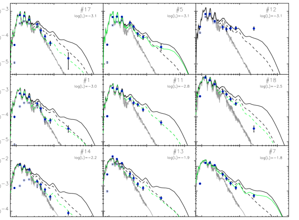
Figure 5: SEDs with stellar atmosphere and disk models for $\rm{log}(L_{\ast}/L_{\odot}){\leq}-1.8$. In each panel, the blue open and filled circles show the observed and dereddened data, respectively. The grey solid line shows the SED of the stellar atmosphere model (Allard et al. 2001; Hauschildt et al. 1999). The stellar atmospheres shown here have the values of T_eff and log($g$) listed in Table 6, and are superposed (not fit) onto the data for the cloud distances listed in Table 2. The black solid line is the predicted SED of a face-on, flared disk with an inner radius equal to the stellar radius ($R_{i}=R_{\ast}$). The black dashed line is the predicted SED of a face-on, flat disk with $R_{i}=R_{\ast}$. The green line denotes the best fit to the data and is solid for flared disk models and dashed for flat disk models, as listed in Table 6. Source $\#$11 is best-fit by a flat, face-on disk with $R_{i}=R_{\ast}$. Increased inner radii are required for $\#$1 ($R_{i}=4$ $R_{\ast}$) and $\#$13 ($R_{i}=3$ $R_{\ast}$). Inclined disks with $R_{i}=R_{\ast}$ are required for $\#$5, $\#$7, and $\#$18 ($i=60^{o}$). Inclined disk ($i=60^{o}$) with large inner radii ($R_{i}=3$ $R_{\ast}$) are required for $\#$14 and $\#$17.

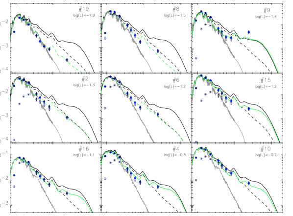
Figure 6: SEDs with stellar atmosphere and disk models for $\rm{log}(L_{\ast}/L_{\odot}){\geq}-1.8$. Symbols and lines are as in Figure 5. Increased inner radii ($R_{i}=3$ $R_{\ast}$) are required for $\#$2 and $\#$6. Inclined disks ($i=60^{o}$) with $R_{i}=R_{\ast}$ are required for $\#$8, $\#$10, $\#$15, and $\#$16. Inclined disks ($i=60^{o}$) with large inner radii are required for $\#$4 ($R_{i}=3$ $R_{\ast}$), $\#$9 ($R_{i}=10$ $R_{\ast}$) and $\#$19 ($R_{i}=5$ $R_{\ast}$).

Figure 8: The ratio of excess emission to central source luminosity increases for lower luminosity sources. Upper Panel: Luminosity of the central source vs. the ratio of the IRAC3 through MIPS1 excess luminosity to the central source luminosity. The dotted line shows a linear fit to our data points and the dashed line shows a linear fit excluding sources #12 and #3. Typical uncertainties (shown in the upper right) are 0.2 dex in luminosity and 0.15 dex in the excess to central source luminosity (see §3.2 for a discussion of uncertainties). Lower Panel: Luminosity of the central source vs. the ratio of IRAC4 excess luminosity to the central source luminosity. The triangles show sources having i-band magnitudes from Natta et al. (2002) and the squares show Cha 1109-7734 and OTS44 (Luhman et al. 2005b, c). We calculated the luminosities and excesses using the method outlined in §3.2. For the Natta et al. (2002) sources, we obtained near-IR fluxes from the 2MASS catalog and IRAC fluxes from the c2d survey of the Ophiuchus cloud core (Allen et al. 2006, in preparation).

References

- Alcala et al. (1997) Alcalá, J. M., Krautter, J., Covino, E., Neuhaeuser, R., Schmitt, J. H. M. M., & Wichmann, R. 1997, A&A, 319, 184
- Alcalá et al. (2000) Alcalá, J. M., Covino, E., Sterzik, M. F., Schmitt, J. H. M. M., Krautter, J., & Neuhäuser, R. 2000, A&A, 355, 629
- Allard et al. (2001) Allard, F., Hauschildt, P. H., Alexander, D. R., Tamanai, A., & Schweitzer, A. 2001, ApJ, 556, 357
- Baraffe et al. (1998) Baraffe, I., Chabrier, G., Allard, F., & Hauschildt, P. H. 1998, A&A, 337, 403
- Baraffe et al. (2002) Baraffe, I., Chabrier, G., Allard, F., & Hauschildt, P. H. 2002, A&A, 382, 563
- Baraffe et al. (2003) Baraffe, I., Chabrier, G., Barman, T. S., Allard, F., & Hauschildt, P. H. 2003, A&A, 402, 701
- Bertin & Arnouts (1996) Bertin, E., & Arnouts, S. 1996, A&AS, 117, 393
- Burgasser et al. (2004) Burgasser, A. J., Kirkpatrick, J. D., McGovern, M. R., McLean, I. S., Prato, L., & Reid, I. N. 2004, ApJ, 604, 827
- Briceño et al. (2002) Briceño, C., Luhman, K. L., Hartmann, L., Stauffer, J. R., & Kirkpatrick, J. D. 2002, ApJ, 580, 317
- Cambrésy (1999) Cambrésy, L. 1999, A&A, 345, 965
- Chauvin et al. (2004) Chauvin, G., Lagrange, A.-M., Dumas, C., Zuckerman, B., Mouillet, D., Song, I., Beuzit, J.-L., & Lowrance, P. 2004, A&A, 425, L29
- Chiang & Goldreich (1997) Chiang, E. I., & Goldreich, P. 1997, ApJ, 490, 368
- Cieza et al. (2005) Cieza, L. A., Kessler-Silacci, J. E., Jaffe, D. T., Harvey, P. M., & Evans, N. J. 2005, ApJ, 635, 422
- D’Antona & Mazzitelli (1994) D’Antona, F., & Mazzitelli, I. 1994, ApJS, 90, 467
- Dahn et al. (2002) Dahn, C. C., et al. 2002, AJ, 124, 1170
- de Geus et al. (1989) de Geus, E. J., de Zeeuw, P. T., & Lub, J. 1989, A&A, 216, 44
- Dullemond et al. (2001) Dullemond, C. P., Dominik, C., & Natta, A. 2001, ApJ, 560, 957
- Drory et al. (2001) Drory, N., Feulner, G., Bender, R., Botzler, C. S., Hopp, U., Maraston, C., Mendes de Oliveira, C., & Snigula, J. 2001, MNRAS, 325, 550
- Evans et al. (2003) Evans, N. J., II, et al. 2003, PASP, 115, 965
- Evans et al. (2005) Evans, N. J., II, et al. 2005, Third Delivery of Data from the c2d Legacy Project, (Pasadena: Spitzer Science Center), http://ssc.spitzer.caltech.edu/legacy/
- Fazio et al. (2004) Fazio, G. G., et al. 2004, ApJS, 154, 10
- Fiorucci & Munari (2003) Fiorucci, M., & Munari, U. 2003, A&A, 401, 781
- Fitzpatrick (1999) Fitzpatrick, E. L. 1999, PASP, 111, 63
- Golimowski et al. (2004) Golimowski, D. A., et al. 2004, AJ, 127, 3516
- Greene & Meyer (1995) Greene, T. P., & Meyer, M. R. 1995, ApJ, 450, 233
- Haisch et al. (2001) Haisch, K. E., Lada, E. A., & Lada, C. J. 2001, ApJ, 553, L153
- Hauschildt et al. (1999) Hauschildt, P. H., et al. 1999, ApJ, 525, 871
- Hartigan (1993) Hartigan, P. 1993, AJ, 105, 1511
- Hartmann (1998) Hartmann, L. 1998, Accretion processes in star formation (Cambridge: Cambridge Univ. Press)
- Harvey et al. (2006) Harvey, P. M, et al. 2006, ApJ, submitted
- Hillenbrand & White (2004) Hillenbrand, L. A., & White, R. J. 2004, ApJ, 604, 741
- Hughes & Hartigan (1992) Hughes, J., & Hartigan, P. 1992, AJ, 104, 680
- Hughes et al. (1994) Hughes, J., Hartigan, P., Krautter, J., & Kelemen, J. 1994, AJ, 108, 1071
- Jayawardhana et al. (2003) Jayawardhana, R., Ardila, D. R., Stelzer, B., & Haisch, K. E. 2003, AJ, 126, 1515
- Lada et al. (2004) Lada, C. J., Muench, A. A., Lada, E. A., & Alves, J. F. 2004, AJ, 128, 1254
- Landolt (1992) Landolt, A. U. 1992, AJ, 104, 340
- Laor & Draine (1993) Laor, A., & Draine, B. T. 1993, ApJ, 402, 441
- Liu et al. (2003) Liu, M. C., Najita, J., & Tokunaga, A. T. 2003, ApJ, 585, 372
- Lucas et al. (2001) Lucas, P. W., Roche, P. F., Allard, F., & Hauschildt, P. H. 2001, MNRAS, 326, 695
- Lucas et al. (2005) Lucas, P. W., Roche, P. F., & Tamura, M. 2005, MNRAS, 361, 211
- Luhman (2004) Luhman, K. L. 2004, ApJ, 602, 816
- Luhman et al. (2005a) Luhman, K. L., et al. 2005, ApJ, 631, L69
- Luhman et al. (2005b) Luhman, K. L., Adame, L., D’Alessio, P., Calvet, N., Hartmann, L., Megeath, S. T., & Fazio, G. G. 2005, ApJ, 635, L93
- Luhman et al. (2005c) Luhman, K. L., D’Alessio, P., Calvet, N., Allen, L. E., Hartmann, L., Megeath, S. T., Myers, P. C., & Fazio, G. G. 2005, ApJ, 620, L51
- Luhman et al. (2004) Luhman, K. L., Peterson, D. E., & Megeath, S. T. 2004, ApJ, 617, 565
- Luhman & Rieke (1999) Luhman, K. L., & Rieke, G. H. 1999, ApJ, 525, 440
- Marley et al. (2002) Marley, M. S., Seager, S., Saumon, D., Lodders, K., Ackerman, A. S., Freedman, R. S., & Fan, X. 2002, ApJ, 568, 335
- Monet (1998) Monet, D. G. 1998, BAAS, 30, 5
- Muench et al. (2001) Muench, A. A., Alves, J., Lada, C. J., & Lada, E. A. 2001, ApJ, 558, L51
- Muller et al. (1998) Muller, G. P., Reed, R., Armandroff, T., Boroson, T. A., & Jacoby, G. H. 1998, Proc. SPIE, 3355, 577
- Muzerolle et al. (2005) Muzerolle, J., Luhman, K. L., Briceño, C., Hartmann, L., & Calvet, N. 2005, ApJ, 625, 906
- Natta & Testi (2001) Natta, A., & Testi, L. 2001, A&A, 376, L22
- Natta et al. (2002) Natta, A., et al. 2002, A&A, 393, 597
- Palla & Stahler (1999) Palla, F., & Stahler, S. W. 1999, ApJ, 525, 772
- Patten et al. (2004) Patten, B. M., et al. 2004, BAAS, 36, 5
- Persi et al. (2003) Persi, P., Marenzi, A. R., Gómez, M., & Olofsson, G. 2003, A&A, 399, 995
- Prato et al. (2003) Prato, L., Greene, T. P., & Simon, M. 2003, ApJ, 584, 853
- Probst et al. (2003) Probst, R. G., et al. 2003, Proc. SPIE, 4841, 411
- Rieke et al. (2004) Rieke, G. H., et al. 2004, ApJS, 154, 25
- Saumon et al. (1996) Saumon, D., Hubbard, W. B., Burrows, A., Guillot, T., Lunine, J. I., & Chabrier, G. 1996, ApJ, 460, 993
- Schechter et al. (1993) Schechter, P. L., Mateo, M., & Saha, A. 1993, PASP, 105, 1342
- Schwartz (1977) Schwartz, R. D. 1977, ApJS, 35, 161
- Simons & Tokunaga (2002) Simons, D. A., & Tokunaga, A. 2002, PASP, 114, 169
- Valdes (1997) Valdes, F. 1997, Astronomical Society of the Pacific Conference Series, 125, 455
- van der Bliek et al. (2004) van der Bliek, N. S., et al. 2004, Proc. SPIE, 5492, 1582
- Vuong et al. (2001) Vuong, M. H., Cambrésy, L., & Epchtein, N. 2001, A&A, 379, 208
- Walker et al. (2004) Walker, C., Wood, K., Lada, C. J., Robitaille, T., Bjorkman, J. E., & Whitney, B. 2004, MNRAS, 351, 607
- Werner et al. (2004) Werner, M. W., et al. 2004, ApJS, 154, 1
- Whittet et al. (1997) Whittet, D. C. B., Prusti, T., Franco, G. A. P., Gerakines, P. A., Kilkenny, D., Larson, K. A., & Wesselius, P. R. 1997, A&A, 327, 1194
- Wichmann et al. (1997) Wichmann, R., Krautter, J., Covino, E., Alcala, J. M., Neuhaeuser, R., & Schmitt, J. H. M. M. 1997, A&A, 320, 185
- Wilking et al. (2004) Wilking, B. A., Meyer, M. R., Greene, T. P., Mikhail, A., & Carlson, G. 2004, AJ, 127, 1131
- Wilking et al. (2005) Wilking, B. A., Meyer, M. R., Robinson, J. G., & Greene, T. P. 2005, AJ, 130, 1733
- Wilking et al. (1987) Wilking, B. A., Schwartz, R. D., & Blackwell, J. H. 1987, AJ, 94, 106
- Young et al. (2005) Young, K. E., et al. 2005, ApJ, 628, 283
- Zapatero Osorio et al. (2002) Zapatero Osorio, M. R., Béjar, V. J. S., Martín, E. L., Rebolo, R., Barrado y Navascués, D., Mundt, R., Eislöffel, J., & Caballero, J. A. 2002, ApJ, 578, 536