Turbulent Velocity Fields in SPH–simulated Galaxy Clusters: Scaling Laws for the Turbulent Energy

Abstract

We present a study of the turbulent velocity fields in the Intra Cluster Medium of a sample of 21 galaxy clusters simulated by the SPH–code Gadget2, using a new numerical scheme where the artificial viscosity is suppressed outside shocks. The turbulent motions in the ICM of our simulated clusters are detected with a novel method devised to better disentangle laminar bulk motions from chaotic ones. We focus on the scaling law between the turbulent energy content of the gas particles and the total mass, and find that the energy in the form of turbulence scales approximatively with the thermal energy of clusters. We follow the evolution with time of the scaling laws and discuss the physical origin of the observed trends. The simulated data are in agreement with independent semi–analytical calculations, and the combination between the two methods allows to constrain the scaling law over more than two decades in cluster mass.

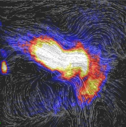
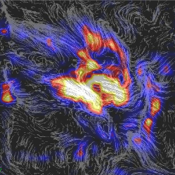
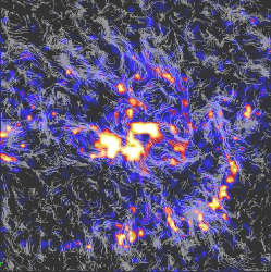
Figure 1: 2–dimensional maps for the central $\sim(1.3\rm{Mpc})^{2}$ region of the most massive cluster of our sample. A subcluster ten times less massive is being accreted (entering from the left). The streamlines on the left depict the velocity defined with respect to the center of mass velocity; on the right depict the local velocity residuals for two different resolutions of the algorithm: $l\sim 32\rm{kpc}$ (center) and $l\sim 16\rm{kpc}$(right). The overlayed colour maps show the kinetic energy of gas particles for each of the velocity fields.

1 Introduction

A good deal of evidence from observational and numerical works is suggesting that a non negligible budget of turbulent motions is stored in the Intra Cluster Medium (ICM) of galaxy clusters. The observational evidence from the gas pressure map of the Coma cluster (Schuecker et al. 2004), the lack of resonant scatterings in Perseus (Churazov et al. 2004), and the many indications of non–thermal emissions possibily due to acceleration of particles into a turbulent magnetized medium (e.g. Brunetti et al.2004 and references therein for a review), are pointing towards the relevance of chaotic motions within the ICM. Moreover, Eulerian numerical simulations of merging clusters (e.g., Bryan & Norman 1998; Roettiger, Stone & Burns 1999; Ricker & Sarazin 2001) or of accretions of less massive structures as dwarf galaxies (e.g. Mayer et al. 2005) have provided good representations of the way in which turbulence may be injected into the ICM. Also theoretical calculations expect a non–negligible amount of turbulent motions in galaxy clusters (e.g. Cassano & Brunetti 2005, C&B05), possibly with a relevant amplification of seed magnetic fields through kinetic dynamo–effects (e.g. Subramanian, Shukurov & Haugen 2005; Enßlin & Vogt 2005; Schekochihin & Cowley 2006). Even the claim against turbulence in the ICM of some observed galaxy clusters as Perseus (e.g. Fabian et al. 2003) actually rule out only scenarios of very strong turbulence, i.e. with an energy density in turbulence not far from the thermal support.

Unluckily, due to the abrupt breaking of the main instrument onboard of the Astro-E2 mission, the direct detection of turbulent fields through the broadening of iron lines profile (e.g. Inogamov & Sunyaev 2003) has to be postponed to the future. From the numerical viewpoint, Smoothed–Particles–Hydrodynamics (SPH) represents a unique tool to investigate the physics of both the collisional (gas) and non collisional (dark matter - DM) mass components of galaxy clusters; moreover, the high dynamic coverage of SPH permits to study a large interval of cluster sizes, and allows one to follow the evolution of the most interesting features with cosmic time. In this Letter we present the first results from a quest for turbulent velocity fields in a sample of well-tested SPH simulated galaxy clusters (Sec. 2); so far, this is the first time that a fully cosmological and highly resolved set of simulations is employed to search and characterize ICM turbulence. To this end we developed a novel approach to the problem of disentangling bulk motions of gas particles from chaotic ones (Sec. 3); in Dolag et al. 2005 (hereafter Do05) we claimed that such method is more efficient than only removing the cluster bulk velocity as usually done in literature (e.g. Bryan & Norman 1998), allowing one to focus only on the most chaotic part of the ICM flow. In this Letter we focus on the scaling relation between the thermal energy content of simulated galaxy clusters and their kinetic energy in the form of turbulent motions (Sec. 4) and finally compare our findings with the expectations from semi–analytical calculations (Sec. 5).

2 The sample of simulated clusters.

The detailed information about our cluster sample can be found in Do05. It consists of 9 resimulations with 21 galaxy clusters and groups simulated with the tree N-body–SPH code Gadget2 (Springel 2005), performed several times with different physical processes. The cluster regions were extracted from a dark matter only simulation with box of $479\,h^{-1}$Mpc on a side and in the context of a $\Lambda$CDM model with $\Omega_{0}=0.3$, $h=0.7$, $\sigma_{8}=0.9$ and $\Omega_{\rm b}=0.04$ (Yoshida, Sheth & Diaferio 2001). Adopting the ‘Zoomed Initial Conditions’ technique (Tormen, Bouchet & White 1997) the regions were re–simulated in order to achieve higher mass and force resolution. Particle mass for the resimulations is $m_{\mathrm{DM}}=1.13\times 10^{9}\,h^{-1}M_{\odot}$ and $m_{\mathrm{gas}}=1.7\times 10^{8}\,h^{-1}M_{\odot}$; the gravitational softening adopted is $h_{i}\simeq 5\,h^{-1}$kpc (Plummer equivalent between $z=5$ and $z=0$ and kept fixed in comoving units at higher redshits; this also marks the minimum value for smoothing the gas particles within the SPH algorithm).

Here we used all the 21 haloes having virial masses in the range $M_{\rm{vir}}=5.3\cdot 10^{13}-2.3\cdot 10^{15}M_{\odot}\cdot h^{-1}$ found in the set of simulations. They are resolved by $8\cdot 10^{4}$ to $4\cdot 10^{6}$ gas and DM particles respectively. Even if the whole sample allows one to study the role of plasma conductivity, cooling, star formation and feedback processes, we restricted so far to a non-radiative SPH subset where an improved recipe for the numerical viscosity of gas–particles is used. This recipe, which follows an idea of Monaghan & Morris (1997) manages to reduce the amount of numerical, and therefore un–phyisical dissipation of chaotic motions, ensuring at the same time a good treatment of shocked features; its use is mandatory for any study of the chaotic part of the ICM dynamics, since otherwise the standard SPH scheme greatly suppresses any chaotic motion at the smallest scales, even in absence of shocks. For a more detailed discussion about this method we address the reader to Do05.

3 Detection of turbulent motions.

In order to characterize turbulent velocity fields in a fluid medium, the crucial point is to extract a pattern of velocity fluctuations from a complex distribution of velocities. The most used approach in the literature (e.g. Norman & Bryan 1998; Sunyaev, Norman & Bryan 2003) is simply to use individual velocities of the gas particles after subtracting of the mean velocity, computed within a fixed volume. Although this method has been widely employed in many previous works, which indeed found a remarkable level of turbulence within simulated ICM, it can turn out to be highly misleading in the case of substructure crossing the cluster volume. As shown in the left panel of Fig. 1, the motion of a subcluster usually tracks laminar velocity patterns which can differ from the mean virial velocity. This provides a spurious contribution to the estimated turbulent energy, whereas the only correct contribution to consider is the chaotic velocity field at the interface layer with the resident ICM of the primary cluster and along the tail of the subcluster. In order to improve on this we conceived an algorithm which disentangles the chaotic part of the flow in a more effective way. We defined a mean local velocity field $\bf{v}_{\rm{cell}}$ in a cell by interpolating the velocity and density of each gas particle onto a regular mesh using a Triangular Shape Cloud (TSC) window function. The dependence of the mesh–spacing to the final results is discussed in section 4. We then evaluated the local velocity fluctuations of each gas particle by:

$$\bf{\delta v}_{\rm{i}}\simeq\bf{v}_{\rm{i}}-\bf{v}_{\rm{cell}},$$ (1)

where $\bf{v}_{\rm{i}}$ is the 3–dimensional particle velocity, $\bf{v}_{\rm{cell}}$ is the local mean velocity field of the cell where each particle falls. This field obviously varies depending on the choice of grid size: the subtraction of a local velocity field is expected to progressively filter out the contribution from laminar bulk–flows produced by the gravitational infall (which is certainly relevant, for any redshift and all distances from the cluster center, e.g. Tormen, Moscardini & Yosida 2004). Figure 1 gives an example of the velocity fields obtained by subtracting the mean bulk velocity (left panel) and after subtracting the local mean velocity found by our new algorithm for two representative resolutions of the TSC algorithm (middle and right panel). The laminar flow at the largest scales is filtered out by the TSC–kernel, while the most chaotic and swirling flows are highlighted, even though some of the biggest vortices might also have been filtered out. We stress here that this method is just a zero–order approximation: an accurate spectral analysis for turbulent dynamics within the simulated ICM will require further improvements, since the ICM is likely characterized by multiple energy injections (from mergers and accretions) driven simultaneously from different scales.

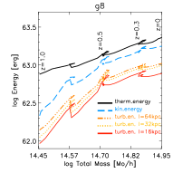
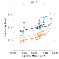
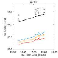
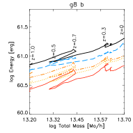
Figure 2: Individual paths for fours clusters of the sample, in the $\log\rm{Energy}-\log\rm{M_{\rm{tot}}}$ plane. The upper two panels show the evolution of the most and of the less massive cluster within our catalogue, whereas the lower two panels show the evolution of two clusters with a nearly equal final mass ($\simeq 5\times 10^{13}M_{\odot}h^{-1}$), but very different “relaxation” state: left panel is for the “relaxed” (i.e. $\xi<0.5$ at z=0) cluster g914 while the right one is for the “perturbed” one, g8 b ($\xi\geq 0.5$ at z=0).

4 Scaling laws for Turbulent Kinetic Energy

The main goal of this section is to investigate the scaling laws between the mass (gas plus dark matter particles) of clusters/groups, $M_{\rm{tot}}$, and the thermal, kinetic and turbulent energy of the ICM.

Due to computational limitations we so far restricted our analysis to a cubic region, centered onto the center of the cluster, of equivalent volume $V_{\rm{box}}=(R_{\rm{vir}})^{3}$. This ensures that we consider in any case a number of gas particles ranging from several thousands to nearly one million. After the velocity decomposition is performed (section 3), we evaluate the turbulent energy content as:

$$E_{\rm{TUR}}=\frac{1}{2}m_{\rm{gas}}\sum_{\rm{BOX}}\delta v_{i}^{2}$$ (2)

where the sum is done over the module of the velocity fluctuation, $\delta v_{i}$, of the gas particles. This calculation was repeated at three different resolutions of the TSC–kernel used to define the local mean velocity field: $l=$16, 32 and 64 kpc. As discussed in Do05 a reasonable subtraction of the laminar pattern is obtained with a mesh spacing around $\sim 30$kpc (corresponding to a TSC equivalent length three times larger).

The total kinetic and thermal energies were evaluated as:

$$E_{\rm{TH}}=\frac{3}{2}m_{\rm{gas}}\sum_{\rm{BOX}}\frac{f_{e}k_{B}T_{i}}{\mu m_{p}},$$ (3)

where $k_{B}$ is Boltzmann’s constant, $T_{i}$ the gas particle temperature, $\mu=0.59$ the mean molecolar weight in AMU, $m_{p}$ the proton mass and $f_{e}=0.58$ the fraction of free electrons per molecule, assuming a primordial mixture of $x_{H}=0.76$, and

$$E_{\rm{K}}=\frac{1}{2}m_{\rm{gas}}\sum_{\rm{BOX}}v_{i}^{2},$$ (4)

where the module of velocity, $v_{i}$, has been reduced to the center of mass velocity frame (as in Norman & Bryan 1998).

In figure 2 we report the time evolution of four representative clusters in our sample in the $E_{\rm{TUR,TH,K}}$–$M_{\rm{tot}}$ plane. The most “relaxed” structures (as the cluster g914, bottom left panel) present a fairly smooth evolution, whereas “perturbed” structures (as g8b and g1f, right panels) show a more complex evolution with episodic jumps in turbulent and kinetic energies, and have a high ratio, $\xi$, between kinetic (and turbulent) and total (thermal plus kinetic) energy. This reflects the significant difference in the ratio between the kinetic and the potential energy of these clusters (e.g. Tormen et al. 1997), which is higher for the perturbed ones.

Since our cluster sample is extracted from re–simulations centered on 9 massive and fairly isolated clusters, smaller systems generally correspond to structures about to be accreted by larger ones. As such, small systems are often perturbed, and this introduces a bias in the dynamical properties of the cluster population. This bias can however be alleviated by restricting our analysis only to the most “‘relaxed” objects in our sample, as we will see below.

In general, we find the following power law scaling between cluster energy (thermal, kinetic or turbulent) and cluster mass:

$$E_{j}\sim A_{j}(\frac{M_{\rm{tot}}}{10^{15}M_{\odot}h^{-1}})^{D_{j}},$$ (5)

with $j=TH$, $K$, $TUR$, and where $A_{j}$ and $D_{j}$ are the zeroth point and the slope of the correlations, respectively.

We find that the scaling of thermal energy with mass is always consistent with that expected in the virial case, $D_{\rm{TH}}\sim 5/3$, while the values of $D_{K}$ and $D_{TUR}$ slightly depend on the number of ”perturbed” small systems included in the analysis. With all system included, the slope of the scaling between turbulent energy and cluster mass is flatter than that between thermal energy and mass by $\sim 0.2$. As we remove more and more small perturbed systems, the turbulent slope steepens toward the thermal value. If we define the ratio $\xi$ between turbulent and thermal energy for each system and redshift, we find that the flattening of the turbulent scaling with respect to the thermal scaling is statistically significant only if objects with $\xi\geq 0.5$ (nine at z=0) are included.

The slopes of the scalings thus obtained are stable and do not depend on the value of the mesh–spacing, $l$, adopted for the subtraction of the laminar motions (Fig. 3), as the maximum difference does not exceed $\Delta D_{\rm TUR}\sim 0.1$ at any redshift.

In addition, the dependence of the turbulent energy on the adopted mesh–spacing confirms the behaviour already presented in Figure 4 of Do05, with $E_{\rm{TUR}}\propto l^{1/2}$.

Table 1: Values for the slopes of the kinetic and turbulent scaling laws at zero redshift, for the whole sample of data and the “relaxed” subsample, with $1\sigma$ errors.

$l$	$D_{\rm TUR}$ (all)	$D_{\rm TUR}$ (relax)	$D_{\rm K}$ (all)	$D_{\rm K}$ (relax)
16 kpc	1.43 $\pm$ 0.06	1.63 $\pm$ 0.04	1.38 $\pm$ 0.04	1.72 $\pm$ 0.03
32 kpc	1.49 $\pm$ 0.04	1.72 $\pm$ 0.01	1.38 $\pm$ 0.04	1.72 $\pm$ 0.03
64 kpc	1.49 $\pm$ 0.03	1.73 $\pm$ 0.05	1.38 $\pm$ 0.04	1.72 $\pm$ 0.03

Finally, Figure 4 shows the redshift evolution of the slopes, $D_{j}$, and of the zero points, $A_{j}$, of the five correlations (Eq. 5). It is clear that the slopes are relatively constant with redshift; this does not change significantly, unless very “perturbed” groups with $\xi\geq 0.5$ (at each z) are considered in the analysis. In this last case a sistematic flattening ($\Delta D_{\rm K,TUR}\sim 0.2$) of the scaling of the kinetic and turbulent energies with cluster mass at low redshift is found: this is caused by the interactions between objects, which makes the smaller systems more and more perturbed as time proceeds.

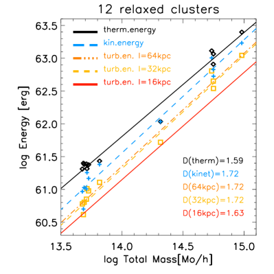
Figure 3: Scaling laws at redshift $z=0$ for the 12 most relaxed clusters ($\xi<0.5$); the values of the slopes for the different relations are reported in the panel. For the sake of displaying, only the datapoints of the $l=32kpc$ grid turbulence are drawn.

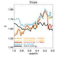
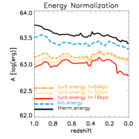
Figure 4: Redshift evolution of slope(left) and zero point (right) of the scaling law Eq.(5), for the sample of objects with $\xi<0.5$.

5 Comparison with semi–analytical results

In the previous section we reported on the scaling between the turbulent energy and the thermal (and kinetic) energy as measured in simulated clusters, without motivating their physical origin. Cluster mergers are likely to be responsible of most of the injection of turbulent velocity fields in the ICM. Simulations have indeed shown that the passage of a massive sub–clump through a galaxy cluster can trigger turbulent velocity fields in the ICM (Roettiger et al.1999; Ricker & Sarazin 2001; Do05).

A simple method to follow the injection of merger–turbulence during cluster life is given by semi–analytical calculations. C&B05 used merger trees to follow the merger history of a synthetic population of galaxy clusters (using the Press & Schechter 1974 model) and calculated the energy of the turbulence injected in the ICM during the mergers experienced by each cluster. In these calculations turbulence is injected in the cluster volume swept by the sub-clusters, which is bound by the effect of the ram pressure stripping, and the turbulent energy is calculated as a fraction of the ${\rm PdV}$ work done by the sub-clusters infalling onto the main cluster.

Although simplified, this semi–analytical approach allows a simple and physical understanding of the scaling laws reported in the previous Section. Indeed, since the infalling sub-clusters are driven by the gravitational potential, the velocity of the infall should be $\sim 1.5-2$ times the sound speed of the main cluster; consequently, the energy density of the turbulence injected during the cluster–crossing should be proportional to the thermal energy density of the main cluster. In addition, the fraction of the volume of the main cluster in which turbulence is injected (the volume swept by the infalling subclusters) depends only on the mass ratio of the two merging clusters, provided that the distribution of the accreted mass–fraction does not strongly depend on the cluster mass (Lacey & Cole 1993). The combination of this two items yields a self–similarity in the injection of turbulence in the ICM: the energy of such turbulence should scale with the cluster thermal energy and the turbulent energy should scale with virial mass with a slope $D_{sem}\sim 1.67$ (C&B05).

In Fig.5 we report the integral of the turbulent energy (injected in the ICM up to the present time) versus the cluster mass, as estimated under the C&B05 approach with 360 merging trees of massive galaxy clusters, together with the measures done on our hydrodynamically simulated clusters: the two scalings are consistent within $1\sigma$ errors. The two approaches are complementary, since semi–analytical calculations can follow the properties of $>10^{15}$M_⊙ clusters which are rare in numerical simulations due to the limited simulated cosmic volume, and so provide a physical extrapolation of the trend derived by our numerical simulations. This strengthens our claim that the turbulent velocity fields detected in simulated clusters are actually real turbulent fields supplied by the mass accretion process acting in galaxy clusters.

Both estimates of the turbulent energy in galaxy clusters show an overall content of turbulence which ranges from 25% to 35% of the thermal one, in the $(R_{\rm{vir}})^{3}$ region. This should be considered as an upper limit of the turbulent energy content at a given time, because simulations do not contain appropriate recipes for the dissipation of the turbulent eddies at the smallest scales (for the sake of comparison, the semi–analytical calculations in Fig.5 were conceived to focus on the injection of turbulence in the whole cluster life).

Fig.5 highlights the different behaviour of “perturbed” (i.e. $\xi\geq 0.5$) and “relaxed” clusters in the turbulent energy – mass plane. As discussed in Section 4 the presence of “perturbed” clusters/groups introduces a bias in the properties of the overall simulated cluster population. In this case the complete sample of our simulations would be more representative of rich environments and superclusters, with the smaller structures beeing more perturbed (and turbulent) than those in other environments. This would cause a systematic flattening of the measured turbulent energy vs mass correlation.

6 Conclusions

Our sample of simulated galaxy clusters shows a well–constrained power–law scaling between the kinetic energy of ICM turbulent motions and the cluster mass. The slope of the scaling does not show any evident dependence on the resolution adopted to detect the pattern of turbulent motions, while the normalization shows a slight dependence on resolution. Rather independently of the cluster mass, the turbulence injected during the cluster life has an energy budget of the order of 25% –35% of the thermal energy at redshift zero. If small perturbed clusters are included in the sample this affects the scaling law of the turbulent energy making it slightly flatter than the thermal case; we expect that this should be the case in supercluster regions. Our scaling is in line with the semi–analytical findings of C&B05: although they used a completely independent method, when plotted together the datapoint of the two approaches prove the scaling over more than two decades in cluster mass. Semi–analytical calculations give a simple physical explanation of the scaling laws in term of the ${\rm PdV}$ work done by the infalling subclusters through the main ones, and strenghten the physical nature of the turbulent field found in simulations. The inclusion of cooling processes within our simulations is not expected to modify our conclusions, because the average cooling time for the large cluster regions considered here is longer than an Hubble time. Cooling may play an important role in innermost regions, where only a minor part of the turbulent energy is stored, however the inclusion of cooling in simulations would also require the implementation of feedback mechanisms – like galactic winds and bubble inflation by AGNs – in order to prevent un–physical massive cooling flows. These processes should also introduce additional turbulence and further studies are required to understand how such processes might effect the reported correlations.

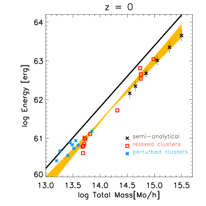
Figure 5: Comparison between the thermal and turbulent scaling at zero redshift, for 12 “relaxed” (i.e. $\xi<0.5$) galaxy clusters, 9 “perturbed” (i.e. $\xi\geq 0.5$) clusters and semi-analytical average data with $1\sigma$ errors. The black line shows the thermal scaling of the whole simulated sample, while the orange band encloses, within $1\sigma$ errors, the scaling of the “relaxed” sample alone and the scaling with the 9 “perturbed” object added.

References

- Brunetti et al. (2004) Brunetti G., Blasi P., Cassano R., Gabici S., 2004, MNRAS, 350, 1174
- Bryan & Norman (1998) Bryan G. L., Norman M. L., 1998, ApJ, 495, 80
- Cassano & Brunetti (2005) Cassano R., Brunetti G., 2005, MNRAS, 357, 1313
- Churazov et al. (2003) Churazov E., Forman W., Jones C., Böhringer H., 2003, ApJ, 590, 225
- Dolag et al. (2005) Dolag K., Vazza F., Brunetti G., Tormen G., 2005, MNRAS, 364, 753
- Ensslin & Vogt (2005) Ensslin T. A., Vogt C., 2005, astro, arXiv:astro-ph/0505517
- Fabian et al. (2003) Fabian A. C., Sanders J. S., Crawford C. S., Conselice C. J., Gallagher J. S., Wyse R. F. G., 2003, MNRAS, 344, L48
- Inogamov & Sunyaev (2003) Inogamov N. A., Sunyaev R. A., 2003, AstL, 29, 791
- Lacey & Cole (1993) Lacey C., Cole S., 1993, MNRAS, 262, 627
- Mayer et al. (2005) Mayer L., Mastropietro C., Wadsley J., Stadel J., Moore B., 2005, astro, arXiv:astro-ph/0504277
- Monaghan & Morriss (1997) Monaghan D. R. J., Morriss G. P., 1997, PhRvE, 56, 476
- Press & Schechter (1974) Press W. H., Schechter P., 1974, ApJ, 187, 425
- Ricker & Sarazin (2001) Ricker P. M., Sarazin C. L., 2001, ApJ, 561, 621
- Roettiger, Stone, & Burns (1999) Roettiger K., Stone J. M., Burns J. O., 1999, ApJ, 518, 594
- Schekochihin & Cowley (2006) Schekochihin A. A., Cowley S. C., 2006, astro, arXiv:astro-ph/0601246
- Schuecker et al. (2004) Schuecker P., Finoguenov A., Miniati F., Böhringer H., Briel U. G., 2004, A&A, 426, 387
- Springel (2005) Springel V., 2005, MNRAS, 364, 1105
- Subramanian, Shukurov, & Haugen (2006) Subramanian K., Shukurov A., Haugen N. E. L., 2006, MNRAS, 99
- Sunyaev, Norman, & Bryan (2003) Sunyaev R. A., Norman M. L., Bryan G. L., 2003, AstL, 29, 783
- Tormen, Bouchet, & White (1997) Tormen G., Bouchet F. R., White S. D. M., 1997, MNRAS, 286, 865
- Tormen, Moscardini, & Yoshida (2004) Tormen G., Moscardini L., Yoshida N., 2004, MNRAS, 350, 1397
- Yoshida, Sheth, & Diaferio (2001) Yoshida N., Sheth R. K., Diaferio A., 2001, MNRAS, 328, 669