Measuring Magnetic Fields in Ultracool Stars and Brown Dwarfs

Abstract

We present a new method for direct measurement of magnetic fields on ultracool stars and brown dwarfs. It takes advantage of the Wing-Ford band of FeH, which are seen throughout the M and L spectral types. These molecular features are not as blended as other optical molecular bands, are reasonably strong through most of the spectral range, and exhibit a response to magnetic fields which is easier to detect than other magnetic diagnostics, including the usual optical and near-infrared atomic spectral lines that have heretofore been employed. The FeH bands show a systematic growth as the star gets cooler. We do not find any contamination by CrH in the relevant spectral region. We are able to model cool and rapidly-rotating spectra from warmer, slowly-rotating spectra utilizing an interpolation scheme based on optical depth scaling. We show that the FeH features can distinguish between negligible, moderate, and high magnetic fluxes on low-mass dwarfs, with a current accuracy of about one kilogauss. Two different approaches to extracting the information from the spectra are developed and compared. Which one is superior depends on a number of factors. We demostrate the validity of our new procedures by comparing the spectra of three M stars whose magnetic fluxes are already known from atomic line analysis. The low and high field stars are used to produce interpolated moderate-strength spectra which closely resemble the moderate-field star. The assumption of linear behavior for the magnetic effects appears to be reasonable, but until the molecular constants are better understood the method is subject to that assumption, and rather approximate. Nonetheless, it opens a new regime of very low-mass objects to direct confirmation and testing of their magnetic dynamos.

1 Introduction

It is generally accepted that magnetic fields are responsible for the generation of solar and stellar activity. In the Sun, magnetic fields can be directly associated with active regions in spatially resolved images. From observations of solar-like stars, the rotation-activity connection was established; the rate of activity grows with faster rotation, which is explained by the rotational sensitivity of a dynamo. In solar-type stars, this dynamo is presumed to lie at the interface between the star’s radiative core and the convective envelope. No break in activity has been found at the transition to fully convective stars, but a different type of dynamo must be working in such cases. The mean level of activity does show a rapid falloff around spectral type M9, even in rapid rotators (Basri & Marcy,, 1995; Mohanty & Basri,, 2003). Some of these objects have extremely low Rossby numbers, for which one could imagine that the dynamo could be inhibited. Magnetic fields in very cool atmospheres are also expected to suffer from very large electrical resistivities and thus efficient field diffusion (Mohanty et al.,, 2002). This can prevent atmospheric motions from being converted into non-radiative heating through magnetic and current dissipation (or MHD wave generation); these mechanisms are thought to be the source of much of the stellar activity in warmer stars.

It has been found that ultracool stars and brown dwarfs of spectral types late M and L can sometimes support low levels of quiescent stellar activity (e.g. Basri,, 2000; Gizis et al.,, 2002; West et al.,, 2004). It is also the case that stellar flares are observed in some of the ultracool objects (e.g. Reid et al.,, 1999; Schmitt & Liefke,, 2002; Liebert et al.,, 2003; Stelzer,, 2004), although they seem to be different than in the solar case, at least in their ratio of radio to X-ray luminosities (e.g. Rutledge et al.,, 2000; Berger,, 2002; Berger et al.,, 2005). In objects M9 and cooler, it is still an open question how much of the observed photometric variability is due to clouds vs. starspots, but H$\alpha$ emission and flaring must be a result of magnetic fields. How is magnetic activity and flaring generated in these objects?

Stellar magnetic fields are usually measured through magnetic Zeeman broadening in atomic lines that have large Landé $g$ values (e.g. Robinson,, 1980; Marcy & Basri,, 1989; Saar,, 2001; Solanki,, 1991; Saar,, 1996, and references therein). The measurement is usually carried out by comparing the profiles of magnetically sensitive and insensitive absorption lines between observations and model spectra. An alternate method that relies on the change in line equivalent widths has also been developed by Basri et al., (1992). Modeling in both cases requires the use of a polarized radiative transfer code and knowledge of the Zeeman shift for each Zeeman component in the magnetic field. Furthermore, it requires the observed lines to be isolated and that they can be measured against a well-defined continuum. The latter becomes more and more difficult in cooler stars since atomic lines vanish in the low-excitation atmospheres and among the ubiquitous molecular lines that appear in the spectra of cool stars. Measurements of stellar magnetic fields extend to stars as late as M4.5 (Johns-Krull & Valenti,, 1996, 2000; Saar,, 2001). In cooler objects, atomic lines can no longer be used for the above-mentioned reasons, and because suitable lines become increasingly rare.

One idea to overcome this problem is to look for Zeeman broadening in molecular lines in ultracool objects. In the sunspot atlas of Wallace et al., (1998), the strong magnetic sensitivity of the Wing-Ford band of FeH just before 1 $\mu$m is clearly demonstrated. Valenti et al., (2001) suggested that FeH would be a useful molecular diagnostic for measuring magnetic fields on ultracool dwarfs, but they point out that improved laboratory or theoretical line data are required in order to model the spectra directly.

In this paper we investigate the possibility of detecting (and measuring) magnetic fields in FeH lines of ultracool dwarfs through comparison between the spectrum of a star with unknown magnetic field strength and spectra of stars for which the magnetic field strength can be calibrated in atomic lines. Such calibrators are generally early- to mid- type M-dwarfs. We explain what sort of data are required at the beginning of §2, then go on to investigate the behavior of the FeH absorption band in stars of different spectral types. A closer look at the magnetic sensitivity of individual FeH lines is accomplished by comparing the spectrum of an active star with a strong magnetic field that was measured in atomic lines to a spectrum of an inactive star that shows no signatures of a magnetic field (§3). Line ratios of magnetically sensitive and insensitive lines are set forth in §4; they are used to determine the detectability of magnetic signatures in stars of different spectral type and rotation velocity. As an example, we determine the magnetic field in a star for which the field is already known from an atomic line analysis using two approaches, FeH line ratios (§4.1) and direct $\chi^{2}$-fitting to the FeH spectrum (§4.2). We give a summary in §5.

2 The Wing-Ford band of FeH in Ultracool Stars

The data we use here were taken during three nights in March and August 2005 with the HIRES spectrograph at Keck I (Vogt et al.,, 1994). The observations were carried out after the detector upgrade, which replaced the previous chip with three new ones. This extends the accessible spectral range and significantly improves the sensitivity in the near infrared. We were able to obtain spectra that cover the wavelength region from H$\alpha$ up to 1 $\mu$m with one exposure, although some gaps occur between the order in the red. Since we observe relatively faint objects along with bright ones, we chose a slit width of 1.15 arcsec, which yields a resolution of $R=31\,000$. We make use of the FeH bands in mid-type M stars, which are relatively bright. The signal-to-noise ratio (SNR) we achieved in those is up to 100 around 1 $\mu$m. The data were reduced using the MIDAS reduction software, they were flat-fielded and filtered for cosmic rays. We subtracted light from sky emission lines by individually extracting the sky spectrum.

Strong absorption around 9900 Å in spectra of M-dwarfs was first observed by Wing & Ford, (1969). Nordh et al., (1977) and Wing et al., (1977) compared spectra of a sunspot and of M-dwarfs to laboratory spectra and assigned the absorption to FeH, and Balfour et al., (1983) established the Wing-Ford band as a ${{}^{4}\Delta}-{{}^{4}\Delta}$ transition of FeH. The rotational analysis of the ${{}^{4}\Delta}-{{}^{4}\Delta}$ system was given by Phillips et al., (1987), and Dulick et al., (2003) provided new line lists and opacities for this system. The band around 9900 Å arises from the $0-0$ $(v^{\prime}-v^{\prime\prime})$ transition of the ${F\,^{4}\Delta}-{X\,^{4}\Delta}$ system. It is already visible in stars of spectral type K5 (Valenti et al.,, 2001) and strengthens through spectral class M to the early L-dwarfs before it fades through the late L dwarfs and early T dwarfs (McLean et al.,, 2003). Fading of the bandhead can be explained by iron condensing out of the atmosphere. The bandhead reappears in early to mid T dwarfs as shown by Burgasser et al., (2002). To explain this strengthening, the authors propose holes to be present in the cloud layer that allow one to see the deeper and hotter layers where FeH is not depleted.

Schiavon et al., (1997) studied the dependence of the Wing-Ford band on model atmosphere parameters, comparing them to medium resolution ($R=13\,000$) spectra of mid-type M stars. Their model spectra match the observed spectra only very coarsely, which may in part be due to their choice of oscillator strengths. Nevertheless, at this resolution, their model seems to produce absorption features at all positions where absorption is visible in the data, thus indicating that FeH is the only major opacity source in that wavelength region. Proceeding towards cooler stars, Cushing et al., (2003) compared low resolution ($R=2000$) spectra of a late-type M and three L dwarfs to a laboratory spectrum of FeH using a King furnace at $T=2700$ K. They identify 34 FeH features that are visible in stellar and laboratory spectra.

We show a high resolution spectroscopic sequence of the Wing-Ford band in the spectral types M2 – L0 in Fig. 1; a detailed investigation of individual features follows in Sect. 3. The strengthening of the absorption features towards later spectral types is clearly visible. Saturation of the strongest lines becomes important after spectral type M5. In cooler objects, even features that are weak in early M-type spectra become comparable to the stronger lines, and eventually fill up the gaps between individual lines. It is not immediately clear whether the saturated spectra of the coolest objects are made up of the same individual absorption features which are discernible in the early M-stars. Our goal is to study the magnetic sensitivity of individual features, which are most evident in spectra of slowly rotating early- to mid-type M stars. In order to extrapolate this method to late-type M stars and even to L-type dwarfs, we have to make sure that the weak absorption features in the early-type M stars are due to the same FeH lines as those in the strong absorption bands in the early L-type dwarfs.

Figure 1: The Wing-Ford band head in objects of spectral types M2 to L0.

In Fig. 2 we show the spectrum of VB 10, an ultracool dwarf of spectral type M8. The strongest FeH absorption features are already severely saturated, while lines that were weak in earlier-type M stars are strong in VB 10. Thus, the difference between strong and weak absorption features of FeH is much smaller than it is in the early-type M dwarfs. In other words, a simple scaling of the strength of absorption features observed in early-type M dwarfs does not yield the absorption pattern observed in a late-type M dwarf, because of spectral line saturation. We find, however, that the pattern is well reproduced if one accounts for saturation, using a scaling that is inspired by scaling optical depth:

$$S(\lambda)=1-C(1-A^{\alpha}).$$ (1)

Here, $A(\lambda)$ is the normalized residual intensity at wavelength $\lambda$ (the original spectrum with the continuum at normalized flux unity). $\alpha$ is the optical depth scale factor which is applied to the entire target spectrum. $C$ is a constant which controls the maximum absorption depth due to saturation (this is necessary to match the cores of strong lines, which do not go to zero, even for large increases in optical depth), and $S(\lambda)$ is the amplified absorption spectrum, weaker FeH absorption can also be calculated using $\alpha<1$. The red line in Fig. 2 shows the spectrum of the M4.5 dwarf GJ 1227 amplified by a factor of $\alpha=3.7$ using a saturation level of $C=0.9$. The amplified spectrum of GJ 1227 matches the strong absorption features in the spectrum of VB 10 remarkably well. It appears that the structure of FeH absorption is identical in the M4.5 dwarf GJ 1227 and in the cooler M8 object VB 10 – one simply sees the effects of increasing saturation of weaker lines in the cooler atmosphere.

We applied the same strategy to 25 objects with spectral types between M2 and L4 and found that in all cases the scaled spectrum of GJ 1227 matches the other FeH spectra very well. The values of $\alpha$ (Eq. 1) that we found for these objects are plotted against their spectral types in Fig. 3. We confirm stronger FeH absorption towards later spectral types among M dwarfs and at spectral type early L, which was shown by McLean et al., (2003) and Cushing et al., (2005). This scaling relation is very helpful when searching for Zeeman broadening in spectra of objects at spectral types for which no reference spectra are available. We can now compare them to scaled versions of spectra of stars with known magnetic fields using the appropriate value of $\alpha$ for that spectral type. It is also very useful for determining rotation velocities (this has to be done first in order to look for Zeeman broadening) in L-type dwarfs, which have no slowly rotating counterparts they could be compared to. The rotation velocity can be directly determined by comparing their FeH spectrum to a scaled spectrum of a slowly rotating mid-type M dwarf. However, a determination of rotation velocities in our ultracool objects is beyond the scope of this paper and we will discuss this topic in more detail in a later paper, in which we also discuss the 25 objects above in more detail.

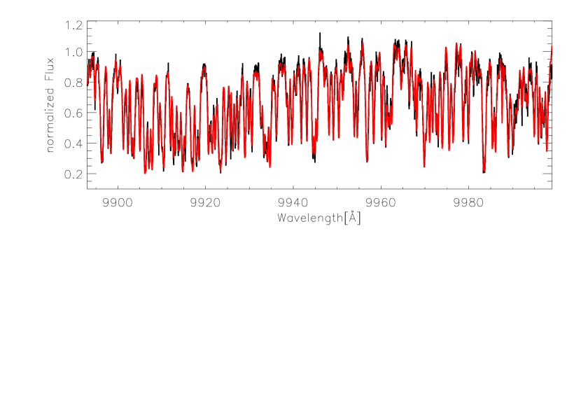
Figure 2: The FeH band in VB10 (M8, black), overplotted with a scaled version of the spectrum of GJ 1227 (red; $\alpha=3.7$, cp. Eq. 1). No rotational broadening was applied.

Figure 3: Scaling of the FeH band in M and L-type objects; the amplification factor $\alpha$ from Eq. 1 is plotted as a function of spectral type.

2.1 CrH absorption in the Wing-Ford band

A second absorption band that falls within the wavelength region of our observation is the $0-1$ band of the $A\,^{6}\Sigma^{+}-X\,^{6}\Sigma^{+}$ system of CrH ($9969\,\mu$m). The detection of this band has been claimed by Burrows et al., (2002) who computed new line lists and opacities. Cushing et al., (2003) question the identification of this CrH bandhead since in their laboratory spectra they found strong FeH features in this region as well. This is in fact important when classifying L dwarfs on the basis of spectral indices (Kirkpatrick et al.,, 1999). From their low-resolution data, Cushing et al., (2003) could not determine to what extent CrH is present around 9970 Å. We show our high resolution spectrum of the slowly rotating M7 object LHS 3003 in Fig. 4 together with a spectrum of the B2IV star $\zeta$ Cas as a telluric reference. Positions of FeH lines from Dulick et al., (2003) are indicated as dashed lines. Absorption features appear at every predicted FeH position. There is only one obvious absorption feature at 9981.0 Å that is apparently not due to FeH, but this comparably small feature does not have a significant influence on the overall opacity. We thus conclude that no CrH absorption is visible in the spectrum of this M7 object. At spectral type M7, absorption in this wavelength interval is entirely caused by FeH. The structure of the band does not change towards early-type L dwarfs (see Fig. 1), which means that even there no evidence for CrH absorption was found.

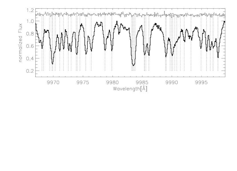
Figure 4: The spectrum of the M7 object LHS 3003 in the region where the CrH band is expected. Overplotted is a telluric reference spectrum of a B2IV star (with an offset of 0.1 for better visibility). Positions of FeH lines are marked with dashed lines; we see no evidence for CrH absorption.

3 Magnetic sensitivity in the FeH band

Magnetic field measurements utilize the space quantization of the atomic angular momentum J in a magnetic field; this is called the Zeeman effect (see for example Solanki,, 1991, and references therein). The sensitivity of atomic absorption lines to a magnetic field is approximately proportional to the Landé factor $g$, which is well known for many transitions. Magnetic splitting in atomic lines can thus be calculated very precisely, and the recent success of radiative transfer models in measuring magnetic fields in cool dwarfs is summarized in Saar, (2001); Valenti & Johns-Krull, (2004).

The molecular Zeeman effect is more complex than the atomic one. The angular momentum vector has more quantization states due to nuclear rotation, which has no dipole moment in the atomic case. The coupling of different angular momenta in the molecule – nuclear rotation, electronic orbit, and electron spin – has to be taken into account. This makes a calculation of the Landé-g factors more difficult than in the atomic case. The coupling can be approximated by Hund’s cases (a) and (b) (e.g. Herzberg,, 1950). A discussion of the molecular Zeeman effect can be found in Crawford, (1934). The couplings of the angular momentum of the ${}^{4}\Delta-^{4}\Delta$ system of FeH is intermediate between the limiting cases (a) and (b) (Phillips et al.,, 1987), but perturbation analysis has not yet been done and spin-orbit coupling constants are still unknown. Berdyugina & Solanki, (2002) show calculations for the Q branch of case (a), the P- and R-branches are zero in this case (lines of the P-, Q- and R-branches have $\Delta J=-1,0,+1$, respectively.). They expect the perturbations to be comparable to the TiO $\gamma$’ system. This means that magnetic sensitivity in the P- and R-branches of FeH lines would be high in transitions with very large values of $J$, and only little around $J\lesssim 15$. In the Q-branch, only the low-$J$ transitions are expected to be magnetically sensitive, since perturbations are less important (Berdyugina & Solanki,, 2002). However, the intermediate coupling of angular momenta makes it difficult to make precise calculations for Landé factors for this molecule, and despite the efforts to understanding the FeH spectrum, its coupling constants have not yet been measured and are still unknown.

In astronomical spectra, strong line broadening has been found in the FeH lines of a sunspot spectrum (Wallace et al.,, 1998). Those authors also investigated the broadening of some lines as a function of $J$. Berdyugina & Solanki, (2002) calculated the behavior of FeH lines for Hund’s case (a) and point out that perturbations appear to be similar to the TiO $\gamma^{\prime}$ system. They find that absolute values of $g_{\rm eff}$ of lines in the R- and P-branches will increase as $J$ increaes. Qualitatively, this is what was observed by (Wallace et al.,, 1998). A clear demonstration of the potential of FeH as a tracer for magnetic fields in cool stars has been given in Valenti et al., (2001). They show that some Zeeman-sensitive lines in the spectrum of the active star AD Leo (M3) are much broader than in the inactive star GJ 725 B (M3.5), while insensitive lines have similar widths. It is obvious that FeH has an excellent potential for measuring magnetic fields in cool dwarfs. However, since coupling constants are still lacking, it is not yet possible to measure magnetic fields by comparison to synthetic spectra. A direct comparison to a sunspot spectrum is also quite dangerous, since in the small spatial area observed, magnetic field lines probably all point towards the same direction. In contrast to the situation in an integrated star spectrum, this means that certain polarization components of the FeH lines may be missing, and the behavior of a sunspot spectrum can significantly differ from the spectrum of a star with a comparable magnetic field. However, a sunspot spectrum could in principle be used to determine empirically Landé–$g$ factors for the upper and lower levels of FeH lines.

Magnetic fields have been measured in early- and mid-type M dwarfs using well-understood atomic lines. In these stars, the FeH band is already prominent as well. For the technique we introduce here, we compare a spectrum of an inactive star which presumably has no measurable magnetic field, and one of an active star with a magnetic field measured from atomic lines, to the spectrum in which we want to detect magnetic broadening. The stars we use are given in Table 1, together with their X-ray and H$\alpha$ activity, and magnetic field measurements from Johns-Krull & Valenti, (2000) if available. In the four panels of Fig. 5, we show the FeH region in our spectra of GJ 1227 (black, inactive star, zero $Bf$) and GJ 873 (red, active star, $Bf=3.9$ kG). The spectral subtypes are slightly different, and the FeH absorption in the cooler star GJ 1227 is a little stronger than it is in GJ 873, which has a slightly higher projected rotation velocity than the former. To make a proper comparison, we amplified the absorption strength in the displayed spectrum of GJ 873 by a factor of $\alpha=1.33$ using Eq. 1, and we artificially broadened the spectrum of GJ 1227 according to a rotational velocity of 4 km s^-1. Above the two M-star spectra, we show the sunspot spectrum of Wallace et al., (1998). The remaining differences in the two non-solar spectra (Gl 873 and GJ 1227) plotted in Fig. 5 are due to the different magnetic fields on the two stars. The spectrum of GJ 1227 shows FeH lines without significant distortion by magnetic fields; all individual absorption lines are narrow. The spectrum of Gl 873 exhibits the effect of magnetic line broadening in a star that has a strong magnetic as well as a non-magnetic component (a filling factor $f$ smaller than 1). The sunspot spectrum shows the extreme case of magnetic broadening with no contribution of the non-magnetic stellar surface outside the spots ($f=1$) and minimal contribution of Zeeman components near line center. This confirms the magnetic nature of the differences between the M stars.

We identified two sets of absorption lines that show different behavior in the magnetic and the non-magnetic cases. Eleven lines that appear relatively insensitive to the Zeeman effect are listed in Table 2; two of them is are blends of two individual lines (we list all lines that contribute to a blend and mark them in the Tables). They are highlighted in blue in Fig. 5. Lines that are particularly sensitive to magnetic fields, i.e., lines that appear significantly different in the two spectra of GJ 1227 and Gl 873, are listed in Table 3 and are highlighted in green in Fig. 5 (four of the features are blends of two lines each). In this paper, we do not investigate the dependence in the magnetic sensitivity of lines with different quantum numbers. Our lists of magnetically insensitive and sensitive lines in Tables 2 and 3 are not comprehensive.

Nevertheless, it easy to see in Table 2 that with very few exceptions, the insensitive lines have $\Omega$ of 0.5 or 1.5, while the sensitive lines have $\Omega$ of 2.5 or 3.5, as expected from the work of Wallace et al., (1998). This confirms the strong dependence of $g_{\rm eff}$ on $\Omega$, the component of the total electronic angular momentum along the internuclear axis. Furthermore, all identified lines that are insensitive to Zeeman broadening belong to the R-branch, most have quantum numbers $J<15$. On the other hand, very sensitive lines were found in all three (R-, P-, and Q-) branches. R-branch lines predominantly have very high $J$-values ($J\sim 20$, but two lines have $J=2.5$), and the two Q-branch lines have very low $J$. Only very few P-branch lines are identified, and only one ($J=15.5$) is not part of a blend. We conclude that magnetic line broading in the stellar spectra is in good agreement with the results from Wallace et al., (1998), namely that magnetic sensitivity strongly depends on the quantum number $\Omega$, a fact that is not accounted for in a standard ${}^{4}\Delta-^{4}\Delta$ Hamiltonian. We also confirm that R-branch lines with very high $J$-values and Q-branch lines with very low $J$-values show strong magnetic sensitivity in qualitative agreement with the predictions from Berdyugina & Solanki, (2002).

A few atomic lines can be seen in this wavelength region as well. In the spectral region of interest, the only atomic lines we expect in the sunspot spectrum and our spectra of late-type M and early-type L dwarfs are the Ti I lines with high oscillator strengths and low excitation; four such lines are in the region between 9900 and 10 000 Å. Two Na I lines may also appear. Line data from the VALD database (Kupka et al.,, 1999) for the six atomic lines are listed in Table 4. Landé $g$ values are only known for the Ti I lines. We mark atomic lines with hatched regions in Fig. 5.

The Wing-Ford band contains a large number of lines that are individually resolved in the spectra of slow rotators. Some of these lines are rather insensitive to a magnetic field, while others show Zeeman broadening that is comparable to rotational broadening on the order of 10 km s^-1. This has the effect of changing the apparent strength of spectral features in a way that is more obvious than the measurement of line broadening. Furthermore, the structure of the FeH band does not vary between ultracool stars with different temperatures so long as the saturation effect is taken into account. Thus the Wing-Ford band provides one of the best opportunities to investigate Zeeman broadening in cool stars and even in late-type M and L dwarfs, at least so long as the signature is not washed out by rapid rotation. The detectability of magnetic fields in cool rotating objects is discussed in the next section.

Table 1: Targets for magnetic field measurements

Name	Sp	log($\frac{L_{\mathrm{X}}}{L_{\mathrm{bol}}}$)	log($\frac{L_{\mathrm{H\alpha}}}{L_{\mathrm{bol}}}$)	$Bf$ [kG]
Gl 729	M3.5e	$-3.50$		2.0
Gl 873	M3.5e	$-3.07$	$-$3.70	3.9
GJ 1227	M4.5	$<-3.85$	$<-5.0$

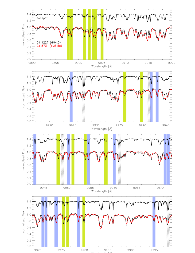
Figure 5: High resolution spectra of the inactive star GJ 1227 (M4.5, lower black line) and the active star Gl 873 (M3.5e). In order to compare the spectra, we artificially enhanced the absorption strength in Gl 873 and spun up the spectrum of GJ 1227 (see text). For comparison, the sunspot spectrum is overplotted with an offset. Magnetically insensitive lines are highlighted in blue, sensitive lines in green. Positions of atomic lines are marked as hatched regions.

Table 2: Magnetically insensitive lines in Fig. 5, these lines are highlighted in blue

$\lambda$ [Å]	Branch	$J$	$\Omega$
9924.6374*	R	6.5	1.5
9924.6374*	R	10.5	3.5
9941.8298	R	9.5	1.5
9943.0934	R	11.5	1.5
9950.3384	R	10.5	1.5
9954.5883	R	12.5	1.5
9960.1308	R	11.5	1.5
9971.0688	R	12.5	1.5
9971.7306	R	4.5	0.5
9973.8550*	R	5.5	0.5
9974.0250*	R	17.5	2.5
9978.7207	R	6.5	0.5
9994.9243	R	7.5	0.5

Table 3: Magnetically very sensitive lines in Fig. 5, these lines are highlighted in green

$\lambda$ [Å]	Branch	$J$	$\Omega$
9897.7737	R	17.5	3.5
9898.4006	R	14.5	3.5
9901.2588	R	18.5	3.5
9902.2715	R	13.5	3.5
9903.1523	R	15.5	3.5
9903.5932	R	14.5	3.5
9905.0208	R	16.5	3.5
9936.0393*	R	2.5	2.5
9936.1883*	R	2.5	2.5
9939.6853*	P	15.5	2.5-3.5
9939.6853*	P	21.5	3.5
9948.0461*	P	10.5	0.5-1.5
9948.1340*	R	23.5	3.5
9951.2732	P	16.5	2.5-3.5
9953.9115	R	22.5	3.5
9958.2533*	R	18.5	2.5
9958.4052*	P	16.5	2.5-3.5
9975.4756	Q	2.5	2.5
9976.3973	R	2.5	0.5
9979.8674	Q	3.5	2.5

Table 4: Atomic lines in ultracool stars^∗

Ion	Wavelength [Å]	J–J	log ($gf$)	Energy levels [eV]	Landé $g$
Ti I	9927.35	4–3	$-$1.580	1.8790 – 3.1280	1.060
Ti I	9941.38	2–3	$-$1.821	2.1600 – 3.4070	1.550
Ti I	9949.00	1–2	$-$1.778	2.1540 – 3.3990	1.510
Ti I	9997.96	3–2	$-$1.840	1.8730 – 3.1130	0.810
Na I	9961.26	2.5–3.5	$-$0.820	3.6170 – 4.8610
Na I	9961.31	1.5–2.5	$-$0.980	3.6170 – 4.8610

4 Detectability of Magnetic Fields on Ultracool Objects

Only very few atomic lines are sufficiently isolated and magnetically sensitive to allow a detection of Zeeman broadening, and often only one spectral line is investigated in studies of magnetic fields in cool stars. In the wavelength region around 1 $\mu$m, however, FeH produces a number of magnetically sensitive and well-isolated lines. The strong signal that is seen in the sensitive FeH lines allows detection of pervasive magnetic fields even in the presence of moderate rotation. In general, one can determine line broadening due to rotation (and perhaps other mechanisms like turbulence) by comparison of magnetically insensitive lines to the same lines in a reference star with known rotational velocity. The Zeeman signal is analyzed by comparing the shape of magnetically sensitive lines between the target spectrum and the reference spectrum. If the Zeeman splitting is small compared to the intrinsic line width, one can only measure the magnetic flux ($Bf$); disentangling the filling factor ($f$) from the magnetic field strength ($B$) is rare in stellar cases (Valenti et al.,, 1995). If the magnetic flux in the reference spectrum is known, one can place limits on the flux in the target spectrum. Having reference spectra for several different flux levels allows refinement of the measurement.

4.1 Magnetic Measurement by Line Ratios

One method of obtaining the magnetic signal is to employ line-depth ratios between magnetically sensitive and insensitive lines. The expectation is that the line-depth ratio between a Zeeman-sensitive and Zeeman-insensitive line depends monotonically on the magnetic field, since the insensitive line remains unaffected while the sensitive line becomes shallower in a stronger field. Such a ratio can be calibrated using reference spectra with known magnetic field strengths.

The two lines should be chosen in close proximity to each other, so that differential errors in continuum placement are less of a concern. Comparing line depths requires the spectra to be observed or broadened to a common resolution. Since rotation and resolution essentially have the same effect on the line widths, the limiting resolution of this method is the one that corresponds to the maximum rotation velocity for which the method can be applied.

We used line-depth ratios to investigate the range of parameters for which a detection of magnetic fields through the FeH Zeeman signal is feasible. We identified four ratios of neighboring absorption features that are particularly useful to measure the magnetic flux – two for slow rotators ($v\,\sin{i}\lesssim 20$ km s^-1) and two for rapid rotators ($v\,\sin{i}\gtrsim 15$ km s^-1). The lines used for these ratios are given in Table 5. For the rapid rotators, the positions are not centered on a physical absorption line, but rather on a feature that is a blend of several lines at that rotation velocity. The Zeeman sensitivity of the blended lines is what we test. In order to investigate the detectability of the Zeeman signal at a given rotation velocity and given spectral type (which has a certain level of saturation), we used the template spectra of active and inactive stars that we have shown in Fig. 5, namely spectra of GJ 1227 (zero field) and Gl 873 ($Bf\sim 3.9$ kG). To probe whether Zeeman broadening due to a field that is weaker than $\sim 4$ kG is detectable, we constructed artificial spectra with intermediate magnetic broadening by a linear interpolation of the observed reference spectra using

$$S_{\rm new}=pS_{\rm Gl\,873}+(1-p)S_{\rm GJ\,1227},$$ (2)

with $S$ the spectra and $p=Bf/(3.9$ kG). This assumes that magnetic broadening is a linear function of $Bf$, which may well not be the case. Especially in the comparison to other stars, a different fraction of surface coverage $f$ will change the structure of line broadening. However, without any knowledge of $f$ and without a detailed modeling of individual Zeeman components, this assumption is probably the best we can do from the observational side. So long as molecular constants are missing, no definite statement about the individual parameters $B$ and $f$ can be made (and even then they may be difficult to disentangle). For now, we have to accept this as a systematic uncertainty of our method.

Table 5: Pairs of magnetically insensitive and magnetically sensitive features used in either slow ($v\,\sin{i}\lesssim 20$ km s^-1) or rapid ($v\,\sin{i}\gtrsim 15$ km s^-1) rotators. The ratio between the depths of two features can be used as a proxy of the magnetic field (see text).

	Insensitive Line	Sensitive Line
	$\lambda$ [Å]	$\lambda$ [Å]
Slow Rotators
1.	9949.11	9948.13
2.	9956.77	9958.25
Rapid Rotators
1.	9948.7	9950.4
2.	9979.8	9978.8

In Fig. 6, we show the predicted behavior of one of the four line ratios of Table 5 with varying magnetic field at different rotation velocities and FeH absorption strength. The sensitive and insensitive features are marked with dashed lines. In the upper row we show the ratio as observed in objects of spectral type M6, i.e., $\alpha=2$. In the lower panel, FeH absorption is saturated and corresponds to a spectral type of L4 ($\alpha=16$). The left column shows spectra in slowly rotating objects, the spectra in the right column are spun up to $v\,\sin{i}=20$ km s^-1. In each panel, five spectra of different “magnetic flux” ($p\sim Bf$) are shown as an example – the top spectra have $p=0$ (pure GJ 1227), the bottom have $p=1$ (pure Gl 873), and the intermediate spectra are linear interpolations of these two cases. In the small figures below each example, we show the ratio of the depths of the magnetically insensitive features to the sensitive features as a function of $Bf=p\cdot 3.9$ kG. It is shown for more points than plotted as examples.

The upper left panel of Fig. 6 shows how the magnetically sensitive line (left marked line) is washed out with growing magnetic field strength while the insensitive line is only marginally affected by the field. The ratio of the two lines, shown in the small figure below, changes from about one in the non-magnetic case to a value of two at $Bf\sim 4$ kG. Such a difference is easily detectable even in data of low SNR. It is no surprise that the two entirely separated lines show monotonic behavior in their interpolated ratio. On the other hand, at faster rotation or in saturated lines, this behavior may be different since blending and saturation wash out the differences between the two measured features. This is shown in the other three panels of Fig. 6. In none of them, the signal is as clear as in the pure case for no rotation without saturation, although the line ratios are still growing with larger field strengths. The amplitude is much smaller than in the pure example.

In Table 5, we have introduced two line ratios that can be used for slow rotators, and two line ratios that are better suited in more rapidly rotating stars. The behavior of all four ratios with varying field strengths are shown for different rotational velocities and different FeH band strengths $\alpha$ (different spectral types) in Figs. 7 and 8; Fig. 7 shows the results for the ratios suited for slow rotators, Fig. 8 shows the ones for rapid rotators. For each case, the left panel shows the first ratio, the right panel shows the second ratio as given in Table 5. For each ratio, six plots are shown in the six rows of Figs. 7 and 8. They correspond to six different values of line depth (Eq. 1), $\alpha\,=\,[0.5,1,2,4,8,16]$, i.e. approximately to the spectral types M3, M4, M6, M8, L1 and L4 (Fig. 3). For the slow rotators, we calculated the ratios for projected rotation velocities of $v\,\sin{i}=[0,5,10,15,20]$ km s^-1, for rapid rotators we show $v\,\sin{i}=[15,20,25,30,35]$ km s^-1, the values of $v\,\sin{i}$ are annotated in the plots.

Most of the ratios shown in Figs. 7 and 8 show a monotonic dependence in $p\sim Bf$, and in many cases magnetic broadening has a detectable influence on these ratios. Thus, magnetic broadening can in principle be detected in objects of spectral type as late as L4 and rotating as rapidly as $v\,\sin{i}=35$ km s^-1. In practice, the limiting factors of such a measurement are the signal-to-noise ratio (SNR) and the determination of the continuum. If strong magnetic broadening in a rapidly rotating object of spectral L4 changes a measured ratio from 1.0 to 1.15, this means that the ratio has to be measurable with such accuracy. In this example, a SNR of 20 would suffice to detect differences between the extreme cases of a field as strong as in Gl 873 ($Bf\approx 4$ kG) and the case of no field. This SNR includes the placement of the continuum, which is especially delicate in rapid rotators where the continuum is no longer visible between individual lines of FeH. This means that the method is more severely limited by the data quality we can achieve, and especially by the accuracy of the rotational velocity one can derive. One can imagine developing more sophisticated techniques to deal with these difficulty cases in the future.

We have obtained a spectrum of another M-dwarf for which the magnetic field strength was measured from atomic lines. The magnetic flux in the M3.5e star Gl 729 is $Bf\approx 2.0$ kG (Johns-Krull & Valenti,, 2000), which is intermediate between the flux found in Gl 873 ($Bf\approx 3.9$ kG) and the zero flux in GJ 1227. We now use its spectrum to check the accuracy of measuring magnetic fields using the line ratios for slow rotators introduced above. For M3.5e the saturation correction factor is about $\alpha=0.9$ (Eq. 1). The projected rotational velocity does not exceed that of GJ 1227, which has a $v\,\sin{i}$ below 2.3 km s^-1 (Delfosse et al.,, 1998). Slow rotation in Gl 729 has also been found by Johns-Krull & Valenti, (1996, $v\,\sin{i}=3.5$ km s^-1).

The ratios most appropriate for Gl 729 are hence the ones for slow rotators, namely the line pairs around 9949 Å and 9957 Å. We measured the ratios between the line depths $d$ in these pairs and find $d$(9949.11Å)/$d$(9948.13Å) = $1.54\pm 0.08$ and $d$(9956.77Å)/$d$(9958.25Å) = $1.61\pm 0.06$. The uncertainties are for a SNR of 100, which is our estimate for the data quality including the determination of the continuum. From these ratios, we can now estimate the value of $Bf$ from the predicted ratios taken from the interpolations in Sect. 4. We have to apply this to the plots in the second top row ($\alpha=1$) of Fig. 7 at the given rotation velocity (we used the region 0–5 km s^-1). The result from the first line ratio is $Bf=(2.45\pm 0.45)$ kG, the second ratio gives $Bf=(1.45\pm 0.80)$ kG. Both values are consistent with $Bf\approx 2.0$ kG as measured from atomic Fe lines, with an error of less than a kilogauss. Furthermore, both values are inconsistent with zero magnetic flux and are also inconsistent with a flux $Bf$ as strong as found on Gl 873 ($Bf\approx 4$ kG). This means, that with the line ratio method in FeH the magnetic flux in Gl 729 can be distinguished from zero flux and from magnetic flux as strong as $Bf=4$ kG.

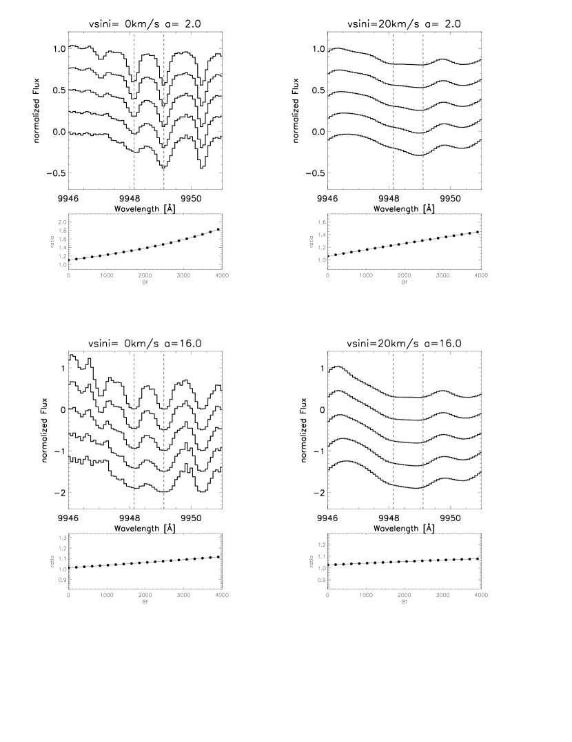
Figure 6: Behavior of the first line pair useful in slow rotators. Left panel shows the case of no rotation, in the right panel the spectra are spun up to $v\,\sin{i}=20$ km s^-1. The upper panel shows the case of non-saturated lines ($\alpha=2,\sim$M6), in the lower panel the FeH band is heavily saturated ($\alpha=16,\sim$L4). In each of the four examples, the magnetic field increases from top to bottom in the spectra. The ratio between the depths of the two absorption features, that are marked with dashed lines, are plotted as a function of $Bf=p\cdot 3.9$ kG in the small plot below each figure (cp Eq. 2).

Figure 7: Depth ratios for slow rotatos; left panel: first ratio; right panel: second ratio. From top to bottom the rows show the results for different absorption strengths of FeH, the approximate spectral type is marked at the left side. In each plot, results for different values with 0 km s${}^{-1}\leq v\,\sin{i}\leq 20$ km s^-1 are given as annotated in the figures.

Figure 8: As Fig. 7 but for the features used in rapid rotators (15 km s${}^{-1}\leq v\,\sin{i}\leq 35$ km s^-1).

4.2 Magnetic Measurement by $\chi^{2}$ fitting

Measuring the magnetic broadening through individual line ratios has a number of weaknesses. Most importantly, line ratios are measured from only a few pixels; in slow rotators the depth of a line may be governed by only one pixel. This means that this method is very prone to noise. Furthermore, the calculation of the line depth seriously depends on the correct placement of the continuum, which may be difficult to determine, particularly in objects of later spectral type that have saturated FeH bands and in rapid rotators. Another caveat to the line-ratio method is that the rotation velocity and FeH absorption strength have to be known in order to translate a ratio to a magnetic field strength. It would be much better to determine all unknown values from a single fit that includes both magnetically sensitive and insensitive lines.

As a second method of measuring the magnetic flux $Bf$ from FeH lines, we construct an artificial spectrum from reference spectra of an inactive star and an active star with known magnetic fields (Eq. 2), and search for the best fit to the spectrum of the object in terms of $\chi^{2}$-fitting. The construction of the spectrum is done by linear interpolation as before. In a first step, we match their continua by simple scaling. Then we search for the best fit to reproduce the target spectrum. The parameters of our fit are FeH saturation strength $\alpha$, projected rotational velocity $v\,\sin{i}$ and magnetic flux $Bf$. With this strategy, all three parameters can be determined simultaneously, and in fact much more accurately, than obtaining them individually. Since lines with different dependencies on the magnetic field are involved, and since the fit is over a significant wavelength region, the result is generally more robust than a determination from one or two line ratios can be. However, any technique that involves $\chi^{2}$-fitting entirely relies on the assumption that a solution exists that can reproduce the data, and that deviations between the data and the fit are essentially due to noise. As soon as systematic differences become important in the calculation of the deviation between data and fit, the results of this technique are difficult to quantify. Thus, it is important to check the reliability of the best fit, i.e., whether it reproduces all significant features – in particular both the magnetically sensitive and insensitive features. If a good fit can be achieved in a broad wavelength region incorporating a number of absoprtion features, this technique will be very sensitive to the magnetic field in terms of $Bf$. Furthermore, if a model can accurately reproduce magnetically sensitive and insensitive lines, there will be little room for systematic problems during the construction of the fit. They should produce significant deviations at least in some of the different features.

As an example, we search for the best fit to our spectrum of Gl 729 using an interpolation between the active star Gl 873 and the inactive star GJ 1227 as done above. We identified four spectral regions that are particularly useful for such a fit in the sense that they contain a number of isolated magnetically sensitive and insensitive lines. The parameters of the stars are given in the previous section and in Table 1. We show the best fit that we achieved in the four panels of Fig. 9; the regions incorporated in the fitting procedure are bracketed with dashed lines. FeH lines that are particularly sensitive to Zeeman broadening are marked in green. The spectrum of the inactive star GJ 1227 (zero $Bf$) is shown as a dashed grey line, the spectrum of the active star Gl 873 ($Bf\approx 3.9$ kG) as a dotted grey line. Our observed spectrum of Gl 729 is plotted in black, it always falls between the two reference spectra. The red line indicates our best fit, it is an interpolation of the two reference spectra with a fraction of 54 % of the active star and 46 % of the inactive star. It provides a remarkably good fit over the whole wavelength region. In particular, the fit can reproduce the data of Gl 729 in all lines that are magnetically sensitive, i.e. where the interpolation lies between the two template spectra. Assuming a linear dependence between line broadening and net magnetic field, one derives a value of $Bf\approx 2.0$ kG. We estimate the uncertainty of the fit by the limits in $Bf$ at which $\chi_{\nu}^{2}=\chi_{\nu,\rm min}^{2}+1$ assuming $\chi_{\nu,\rm min}^{2}=1$, which is the case for a SNR of 90. In other words, we are looking for the values of $Bf$ that yield $\chi_{\nu}^{2}=2$. This yields an an uncertainty of 1.3 kG, i.e., $Bf\approx(2.0\pm 1.3)$ kG.

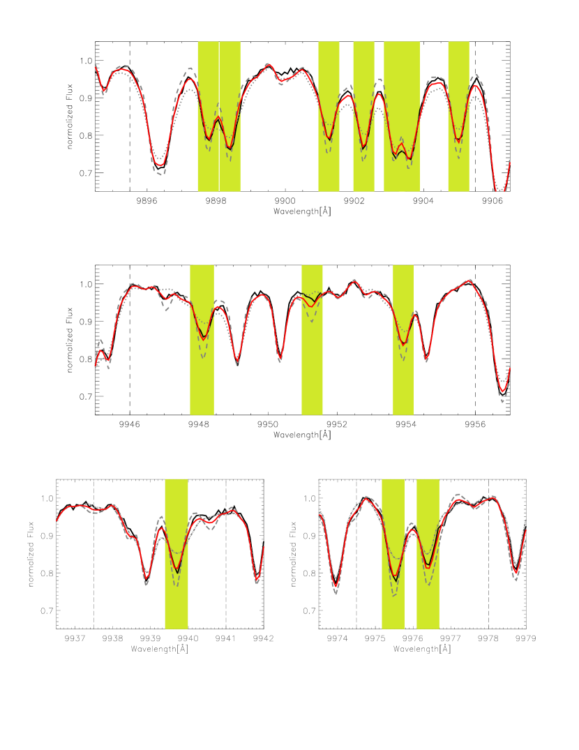
Figure 9: Fit (red line) of a linear interpolation between the spectra of GJ 1227 (grey dashed line) and Gl 873 (grey dotted line) to the spectrum of Gl 729 (black line). $\chi^{2}$ is calculated from the regions between the vertical dashed lines. The best fit is achievd for $Bf=2.0$ kG, i.e. $\sim 50\%$ GJ 1227 and $\sim 50\%$ Gl 873.

4.3 Line ratios vs. data fitting

We have shown two ways of obtaining an estimate of the magnetic flux from Zeeman modification of FeH spectra of cool stars. Both methods rely on the assumption that the spectrum of a star with intermediate magnetic flux can be interpolated between two spectra, one with very weak or zero flux and another with strong flux. Although such an interpolation is not necessarily linear, at this level of accuracy it probably is a reasonable approximation. In practice, the limiting factor of such a measurement is the SNR of the data. This includes the determination of the continuum, which is problematic in spectra of the cooler objects.

Fitting the interpolation of the two template spectra to the data has the advantage that a large part of the spectral region is incorporated and the result is based on a larger number of tracers while anchored in the magnetically insensitive lines. This also yields very precise values of the rotation velocity. However, especially in the cooler stars where FeH is strongly saturated, and in rapid rotators ($v\,\sin{i}\gtrsim 15$ km s^-1), it will be difficult to reach the desired fit quality, mainly because the continuum determination becomes difficult. In this case the value of $\chi^{2}$ becomes meaningless, since no reasonable fit can be achieved at all. Here the line ratios can be more useful since they depend only marginally on the correct placement of the continuum; they focus on a very narrow spectral region. The fact that the errors we get from line ratios are smaller than the one from the $\chi^{2}$-fit is because the formal errors from the line ratio technique do not account for systematic differences between the template and the target spectrum. The true uncertainty including all systematic uncertainties would be larger – these uncertainties are accounted for in the $\chi^{2}$-technique. The two methods introduced in Sects. 4.1 and 4.2 are complementary and we suggest to derive the value of a magnetic field from a direct fit and to check the result using the line ratios. The $\chi^{2}$ method may not be applicable in some cases where line ratios could still provide a reasonable field estimate.

5 Summary

We have analysed high resolution spectra of the FeH Wing-Ford band near 1 $\mu$m in very cool stars. The comparison of absorption features to FeH line lists showed that all significant absorption features around 9980 Å can be assigned to lines of FeH. We did not find extra absorption due to CrH where its 0–1 band was expected. The depth of the FeH absorption lines scales inversely with stellar temperature similar to a “curve of growth” analysis in spectral lines. This makes it possible to predict the spectrum of a rapidly-rotating ultracool object on the basis of spectra of slowly-rotating cool stars, permitting analysis of observed spectra in the late M or L regime. We found that FeH displays a number of spectral lines that are individually resolved and intrinsically narrow, and many of them show significant Landé-g factors. This is a crucial advantage of the FeH Wing-Ford band compared with other molecular bands, whose lines are easily blended by rapid rotation, and which usually have very few magnetically sensitive lines strong enough to be observed. Thus, the lines of the Wing-Ford band provide a unique opportunity to investigate Zeeman broadening, as has been done successfully for decades using atomic lines in hotter stars. It offers the opportunity to extend such studies even to L-type dwarfs, which has not otherwise been possible since slowly rotating L-dwarfs are very rare.

We investigated individual spectral features of the two M-dwarfs GJ 1227 and Gl 873; the latter is a known magnetically active star with a magnetic flux of $Bf\approx 3.9$ kG, while the former is magnetically inactive and does not have a detectable magnetic field. Comparison of the two spectra revealed a number of FeH lines that are particularly sensitive to magnetic broadening – such lines are significantly broader in the magnetically active stars than in the inactive one. Other lines show the same shape in both stars; these lines are not sensitive to magnetic fields and demonstrate that the extra broadening in the sensitive lines cannot be due to rotation or other broadening mechanisms that are universal to all absorption lines.

The molecular constants required for a full calculation of Zeeman broadening in lines of molecular FeH are still unknown, hence Zeeman signatures cannot yet be calculated as a function of magnetic field. In order to measure a magnetic field in ultracool objects, we use spectra of active and inactive stars with known magnetic fields to calibrate the extra broadening seen in lines that are magnetically sensitive. An empirical investigation of four line-depth ratios between magnetically sensitive and magnetically insensitive lines reveals that in principle the effects of Zeeman broadening are detectable in objects of spectral type late M and even in the L regime. Furthermore, magnetic broadening produces signatures strong enough to appear in stars rotating as rapidly as $v\,\sin{i}\approx 30$ km s^-1, although it may be difficult to reach the desired SNR for such a detection, especially in the coolest objects.

In order to test the reliability of the proposed method, we tried to redetermine the magnetic flux of the M3.5e star Gl 729, which is known from measurements in atomic lines. First, we used the line ratios that we calibrated at the spectra of GJ 1227 and Gl 873, and secondly, we fitted an interpolation of these two spectra to the data of Gl 729. Both methods yielded values of $Bf$ that are in reasonable agreement with the field measured in the atomic lines. Most importantly, for both strategies the uncertainties are small enough to significantly exclude the assumption that Gl 729 has no magnetic field, or that it has a field that is as strong as Gl 873. The precision of this method seems to be of the order of 1 kG.

The interpolation of FeH Zeeman signatures from two reference spectra assumes that the magnetic flux signal is a linear function in $Bf$. This assumption is a big simplification of the physical situation, and thus implies that a precise measurement of $Bf$ (and especially a separation of $B$ and $f$) cannot yet be expected from this method. Clearly, a full calculation of the Zeeman splitting in FeH lines would yield much more accuracy in the determination of magnetic fields in cool stars. It is not clear to what extent we could then separate the effects of $B$ and $f$. Nevertheless, until the calculation of molecular Zeeman splitting in FeH becomes achievable, the detection of a magnetic field is by itself very valuable. We can further get a crude idea of what the value of the magnetic flux actually is, and compare stars with broadly different fields. This method provides the first chance of measuring magnetic fields in ultra low-mass stars and brown dwarfs.

References

- Balfour et al., (1983) Balfour, W.J., Lindren, B., & O’Connor, S., 1983, Phys Scr., 28, 551
- Basri et al., (1992) Basri, G., Marcy, G.W., & Valenti, J.A., 1992, ApJ, 390, 622
- Basri & Marcy, (1995) Basri, G., & Marcy, G.W., 1995, AJ, 109, 762
- Basri, (2000) Basri, G. 2000, Eleventh Cool Stars Workshop, A.S.P. CS-223, García-López, Rebolo, & Zapatero-Osorio (Eds.), 261
- Berdyugina & Solanki, (2002) Berdyugina, S.V., & Solanki, S.K., 2002, A&A, 385, 701
- Berger, (2002) Berger, E. 2002,ApJ, 572, 503
- Berger et al., (2005) Berger E., Rutledge, R.E., Reid, I.N., et al., 2005, ApJ, 627, 960
- Burgasser et al., (2002) Burgasser, A.J., Marley, M.S., Ackerman, A.S., et al., 2002, ApJ, 571, L151
- Burrows et al., (2002) Burrows, A., Ram, R.S., Bernath, P., Sharp, C.M., & Milsom, J.A., 2002, ApJ, 577, 986
- Crawford, (1934) Crawford, F.H., 1934, Reviews of Modern Physics, 6, 90
- Cushing et al., (2003) Cushing, M.C., Rayner, J.T., Davis, S.P., & Vacca, W.D., ApJ, 582, 1066
- Cushing et al., (2005) Cushing, M.C., Rayner, J.T., & Vacca, W.D., ApJ, 623, 1115
- Delfosse et al., (1998) Delfosse, X., Forveille, T., Perrier, C., & Mayor, M., 1998, A&A, 331, 581
- Dulick et al., (2003) Dulick, M., Bauschlicher, C.W. Jr., Burrows, A., Sharp, C.M., Ram, R.S., & Bernath, P., 2003, ApJ, 594, 651
- Gizis et al., (2002) Gizis, J.E., Reid, I.N., Hawley, S.L. 2002, AJ, 123, 3356
- Herzberg, (1950) Herzberg, G., 1950., Molecular spectra and molecular structure. Vol.1, Spectra of Diatomic Molecules (2nd ed.; New York, Van Nostrand Reinhold)
- Johns-Krull & Valenti, (1996) Johns-Krull, C., & Valenti, J.A., 1996, ApJ, 459, L95
- Johns-Krull & Valenti, (2000) Johns-Krull, C., & Valenti, J.A., 2000, ASPC, 198, 371
- Kirkpatrick et al., (1999) Kirkpatrick, J.D., Reid, I.N., Liebert, J. et al., 1999, ApJ, 519, 802
- Kupka et al., (1999) Kupka F., Piskunov N.E., Ryabchikova T.A., Stempels H.C., & Weiss W.W., 1999, A&AS, 138, 119
- Liebert et al., (2003) Liebert, J., Kirkpatrick, J.D., Cruz, K.L., Reid, N., Burgasser, A., Tinney, C.G., & Gizis, J.E., 2003, AJ, 125, 343
- Marcy & Basri, (1989) Marcy, G.W., & Basri, G., 1989, ApJ, 345, 480
- McLean et al., (2003) McLean, I.S., McGovern, M.R., Burgasser, A.J., Kirkpatrick, J.D., Prato, L., & Kim, S.S., 2003, ApJ, 596, 561
- Mohanty & Basri, (2003) Mohanty, S., & Basri, G., 2003, ApJ, 583, 451
- Mohanty et al., (2002) Mohanty, S., Basri, G., Shu, F., Allard, F., & Chabrier, G., 2002, ApJ, 571, 469
- Nordh et al., (1977) Nordh, H.L., Lindgren, B., & Wing, R.F., 1977, A&A, 56, 1
- Phillips et al., (1987) Phillips, J.G., Davis, S.P., Lindgren, B., & Balfour, W.J., 1987, ApJ, 65, 721
- Reid et al., (1999) Reid, I.N., Kirkpatrick, J.D., Gizis, J.E., Liebert, J. 1999, ApJ, 527, 105
- Robinson, (1980) Robinson, R.D., 1980, ApJ, 239, 961
- Rutledge et al., (2000) Rutledge, R.E., Basri, G., Martín, E.L., Bildsten, L. 2000, ApJ, 538, 141
- Saar, (1996) Saar, S.H., 1996, in IAU Symp., 176, Stellar Surface Structure, eds., Strassmeier, K., J.L. Linsky, Kluwer, 237
- Saar, (2001) Saar, S.H., 2001, ASPCS 223, 292
- Schiavon et al., (1997) Schiavon, R.P., Barbuy, B., & Singh, P.D., 1997, ApJ, 484, 499
- Schmitt & Liefke, (2002) Schmitt, J.H.M.M., & Liefke, C., 2002, A&A, 382, L9
- Solanki, (1991) Solanki, S.K., 1991, RvMA, 4, 208
- Stelzer, (2004) Stelzer, B., 2004, ApJ, 615, L153
- Valenti et al., (1995) Valenti, J.A., Marcy, G.W., & Basri, G., 1995, ApJ, 439, 939
- Valenti et al., (2001) Valenti, J.A., Johns-Krull, C.M., & Piskunov, N.P., 2001, ASP 223, 1579
- Valenti & Johns-Krull, (2004) Valenti, J. A., & Johns–Krull, C. M., Ap&SS, 292, 619
- Vogt et al., (1994) Vogt, S. S. et al., 1994, Proc. SPIE Instrumentation in Astronomy VIII, David L. Crawford; Eric R. Craine; Eds., 2198, 362
- Wallace et al., (1998) Wallace, L., Livingston, W.C., Bernath, P.F., Ram, R.S., 1998, An Atlas of the Sunspot Umbral Spectrum in the Red and Infrared from 8900 to 15 050 cm-1 (6642 to 11 230 Å), NOAO, ftp://ftp.noao.edu/fts/spot3atl
- West et al., (2004) West, A.A., Hawley, S.L., Walkowicz, L.M., Covey, K.R., Silvestri, N.M., Raymond, S.N., Harris, H.C., Munn, J.A., McGehee, P.M., Ivezic, Z., Brinkmann, J. 2004, AJ, 128, 426
- Wing et al., (1977) Wing, R.F., Cohen, J., & Brault, J.W., 1977, ApJ, 216, 659
- Wing & Ford, (1969) Wing, R.F., & Ford, W.K., 1969, PASP, 81, 527