The redshift sensitivities of dark energy surveys

Abstract

Great uncertainty surrounds dark energy, both in terms of its physics, and the choice of methods by which the problem should be addressed. Here we quantify the redshift sensitivities offered by different techniques. We focus on the three methods most adept at constraining $w$, namely supernovae, cosmic shear, and baryon oscillations. For each we provide insight into the family of $w(z)$ models which are permitted for a particular constraint on either $w=w_{0}$ or $w=w_{0}+w_{a}(1-a)$. Our results are in the form of “weight functions”, which describe the fitted model parameters as a weighted average over the true functional form. For example, we find the recent best-fit from the Supernovae Legacy Survey ($w=-1.023$) corresponds to the average value of $w(z)$ over the range $0<z<0.4$. Whilst there is a strong dependence on the choice of priors, each cosmological probe displays distinctive characteristics in their redshift sensitivities. In the case of proposed future surveys, a SNAP-like supernova survey probes a mean redshift of $z\sim 0.3$, with baryon oscillations and cosmic shear at $z\sim 0.6$. If we consider the evolution of $w$, sensitivities shift to slightly higher redshift. Finally, we find that the weight functions may be expressed as a weighted average of the popular “principal components”.

I Introduction

Following the rapid accumulation of experimental evidence (including Riess et al. (1998); Perlmutter et al. (1999); Riess et al. (2004); Hoekstra et al. (2005); Cole et al. (2005); Lange et al. (2001); Spergel et al. (2003); Allen et al. (2004)), it has become widely accepted that the Universe is experiencing a period of accelerated expansion. In the context of general relativity, this implies that the current cosmological dynamics are dominated by a component with negative pressure. There is currently no satisfactory theoretical explanation despite the proliferation of models that have been suggested. Theories range from vacuum energy, through scalar fields, to modifications of general relativity, although none have yet produced satisfactory solutions to the theoretical issues. By revealing the behavior of this dark energy, not only might we foresee the ultimate fate of the Universe, but this may be the first step into a new field of physics.

Dark energy is often parameterised by its equation of state, the pressure to density ratio $w=p/\rho$. This is believed to summarise the main effect of dark energy on the observable universe. This equation of state is expected to change with time, and therefore redshift (with the notable exception of the cosmological constant).

Since dark energy is generally considered to be the biggest problem facing cosmology today, there are a multitude of proposed surveys which aim to find out more about its nature (summarised in Fig. 1). Decisions need to be made regarding which surveys to carry out, given limited funds. Since the proposed surveys reduce the random uncertainties by more than an order of magnitude, we have to admit the possibility that systematic uncertainties may come to dominate the constraints on dark energy, for some cosmological probes. Unfortunately it is extremely difficult to quantify these systematic uncertainties, and a rigorous treatment of these lie beyond the scope of this paper. We focus on a comparison of three different probes (supernovae, cosmic shear and baryon oscillations), putting them on an equal footing and assessing their theoretical complementarity.

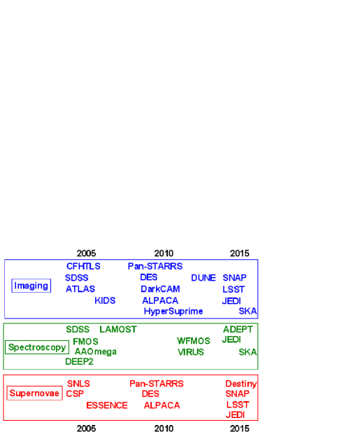
Figure 1: Sketch illustrating the large number of experiments proposing to measure dark energy using the probes discussed in this paper.

Supernova light curves offer the most mature probe of dark energy, with a number of surveys currently in progress. They are used to infer the expansion history through measurements of the luminosity distance, and its variation with redshift.

The gravitational deflection of light slightly warps the images of distant galaxies. These distortions are sensitive to dark energy via the distance-redshift relation, and to a lesser extent by the growth of structure. Current constraints are modest, with an upper bound of $w\lesssim-0.5$ Hoekstra et al. (2005) (roughly $2\sigma$).

Oscillatory features in the galaxy power spectrum have recently been seen by two redshift surveys Eisenstein et al. (2005); Cole et al. (2005). By resolving these with higher precision and over a range of redshifts, competitive constraints on $w$ could be achieved Blake and Glazebrook (2003); Seo and Eisenstein (2003); Blake et al. (2004).

The potential of a particular cosmological probe can be assessed in a variety of ways. The most common approach has been to assume that the dark energy equation of state takes a simple form as a function of redshift, and then the predicted constraints on the parameters of the function are calculated. It is highly challenging for even the ambitious proposed experiments to constrain the detailed evolution of the equation of state. Each probe can typically only give one or two parameters Linder and Huterer (2005); Saini et al. (2004), and therefore the equation of state is often expanded to zeroth or first order in redshift. (Such that $w(z)=w_{0}$ or $w(z)=w_{0}+w_{1}z$ or into the more theoretically motivated form $w(z)=w_{0}+w_{a}(1-a)$ in which the dark energy has a value $w_{0}$ today, and gradually approaches $w_{0}+w_{a}$ toward higher redshift). These constraints are important for comparing the potential of different surveys and probes.

However, it has been realised that the resulting contour plots do not tell the whole story of how sensitive each probe is as a function of redshift, or how many independent pieces of information each will yield on dark energy. The principal component approach assesses both of these points Huterer and Starkman (2003); Knox et al. (2005); Crittenden and Pogosian (2005). This is achieved by attempting to measure the equation of state in narrow bins in redshift, and diagonalising the resulting correlated error matrix.

The weight function approach Deep Saini et al. (2003); Simpson and Bridle (2005) aims to address a slightly different question. It allows us to interpret fitted parameters, such as $w_{0}$, in terms of a weighted redshift average over the true, potentially varying, equation of state. The resulting weight function also gives an impression of the sensitivity of each probe as a function of redshift.

Unfortunately, conclusions on all of the above issues depend on the assumptions made about dark energy and other priors. Priors have to be placed on the other cosmological parameters as well as on the range of possibilities allowed for the dark energy.

Here we attempt to bring all of these issues together and compare the three cosmological probes listed above on an equal basis. We consider the ability of the various probes to disentangle multiple pieces of information on the dark energy using a PCA analysis; and not only do our weight functions look similar to the principal components, but they are simply related. The redshift sensitivities of different probes are compared, in the case of both constant and evolving equation of state parameterisations. The effect of different priors on cosmological parameters is explored. Finally, we assess the bias which can arise when fitting other cosmological parameters.

II Concept

Intuitively one might imagine that slight deviations in $w$ would be reflected by a representative shift of our observed value. However, as we shall see, this is not necessarily the case. A particularly extreme example was highlighted by Maor et al. Maor et al. (2002), in which a quintessence model of $w(z)\geq-0.7$ was shown to provide a best-fit of $w<-1$. This fundamentally arises from (a) the incorrect parameterisation of $w$ and (b) our incomplete knowledge of other cosmological parameters. By improving our data, these effects will be suppressed but never eliminated.

Inevitably, results will emerge which assume a time-independent value for $w$, or at best permitting some pre-determined variation such as $w=w_{0}+w_{a}(1-a)$ Chevallier and Polarski (2001); Linder (2003). The aim here is to provide insight into the meaning of these results, within the context of dark energy actually exhibiting an arbitrary $w(z)$. In doing so, we quantify the redshift sensitivities of different surveys. Central to our approach will be expressing the best-fit value of $w$ as a weighted integral over the true $w(z)$. The key ingredient is the “weight function” $\Phi(z)$ defined such that

$$w^{fit}=\int\Phi(z)w(z)\mathrm{d}z\,\,\,.$$ (1)

This weight function can be interpreted as the redshift-sensitivity of the observation. In principle, $\Phi(z)$ depends on $w(z)$, although we find that in practice the dependence is weak (see Appendix B). In this paper all $\Phi(z)$ functions are calculated using the fiducial model $w(z)=-1$, unless stated otherwise.

To derive the weight functions, we adopt a different path from previous work. This provides greater flexibility, and allows marginalisation over other parameters. We begin by permitting $w$ to adopt an independent value within each infinitesimal redshift bin. The eigenvectors of the resulting Fisher matrix, marginalised over the relevant parameters, provide the ‘principal components’, or eigenmodes, of the survey. These orthonormal functions $e_{i}(z)$ allow us to express $w(z)$ in the form

$$w(z)=\sum_{i}\alpha_{i}e_{i}(z)$$ (2)

such that the errors $\sigma(\alpha_{i})$ are uncorrelated. Further details of this approach are explored by Huterer & Starkman Huterer and Starkman (2003). Weight functions are most readily derived from the principal components (hereafter PCAs) of a given survey. For example, in the case of fitting a constant $w$, using chi-squared minimisation we find

$$\Phi(z)=\frac{\sum_{i}{e_{i}(z)\int e_{i}(z^{\prime})\mathrm{d}z^{\prime}/\sigma^{2}(\alpha_{i})}}{\sum_{j}(\int e_{j}(z^{\prime\prime})\mathrm{d}z^{\prime\prime})^{2}/\sigma^{2}(\alpha_{j})}\,\,.$$ (3)

The weight function $\Phi(z)$ is a sum of the eigenmodes weighted with the strength by which their coefficients are determined, and so is a representation of the sensitivity. For further details see Appendix C. Note that in general, any complete orthonormal set such as these principal components, are their own weight functions.

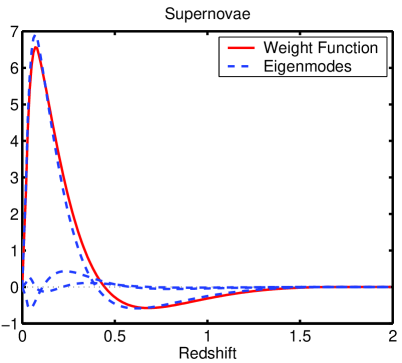
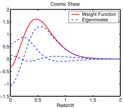
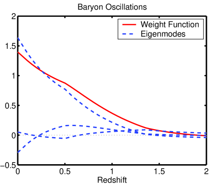
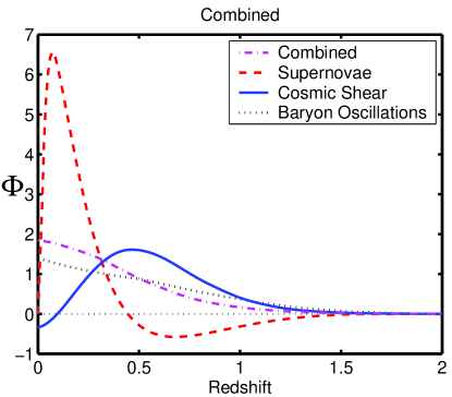
Figure 2: Top left: Supernovae. First three PCA eigenmodes (dashed lines) weighted in accordance with equation (3), the sum of which gives the weight function (solid line) for a constant $w$ fit. For a SNAP-like survey. Top right: Similarly for cosmic shear, whose weight function has significant contributions from the higher modes. For a SNAP-like distribution of source galaxies (weight functions and PCAs are independent of the survey area). Bottom left: Same for baryon oscillations. The weight function is distinctive in its simplicity, with a slight discontinuity in the gradient corresponding to the edge of the lower redshift bin. Survey parameters correspond to the proposed WFMOS survey. Bottom right: Here we superpose the weight functions of the previous plots, allowing for a more detailed comparison. In addition, the dot-dash line represents the sensitivity of a combined analysis.

III The Weight Functions

In this section we consider each of the three main cosmological probes of dark energy, deriving PCAs and weight functions for fitting a constant dark energy equation of state. We vary the main relevant cosmological parameters, marginalising over them with flat priors on each (this improves on our previous work). In section IV we examine the effect of these priors.

A flat universe is assumed throughout this paper. Whilst the possibility of non-zero curvature should not be completely ignored, a flat universe still remains the most likely theoretical option, and will be used to provide the tightest constraints on $w$. Curvature is trivially incorporated into this approach, and the implications for PCAs and weight functions may be explored in future work.

Each of the following subsections briefly summarises the relevant physics, outlines the fiducial survey parameters, and discusses the resulting PCAs and weight functions from Fig. 2. Note that in Appendix A this collection of weight functions are re-expressed in terms of the scale factor rather than redshift.

III.1 Supernovae

Our fiducial survey consists of 2000 supernovae uniformly distributed from $z=0.1-2$, with a further 300 in the range $0.03<z<0.08$, as anticipated from the Nearby Supernova Factory. We calculate the PCAs and weight functions from measurements of the observed magnitudes, $m$,

$$m-\mathcal{M}=5\log_{10}D_{L}$$ (4)

where $\mathcal{M}$ incorporates the intrinsic magnitude and the Hubble parameter, and the redshift dependence of the luminosity distance $D_{L}$ provides our grasp on the equation of state.

We apply a flat prior to the parameters $\mathcal{M}$ and $\Omega_{\rm{m}}$. Following Linder & Huterer Linder and Huterer (2003), we include an irreducible uncertainty of the form $\mathrm{d}m=0.02(1+z)/2.7$ in bins of width $\Delta z=0.1$, to mimic systematics.

The PCA eigenvalues deteriorate quite sharply, and higher modes are penalised for their oscillatory nature, so the weight function looks similar to the first PCA eigenmode. The weight function peaks at around $z\sim 0.1$ and has a smaller negative tail beyond $z>0.45$. We consider the mean of $|\Phi(z)|$ to be a good benchmark, and in this case find a value of 0.28.

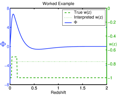
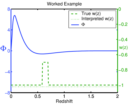
Figure 3: Left: This is an example illustrating the meaning of the weight function. A perturbation in the underlying $w(z)$ model (dashed) leads to a shift in our best fit (dotted) with a magnitude given by the corresponding value of the weight function at that redshift. Right: A similar scenario to Fig. 3, except here the perturbation in the true $w(z)$ (dashed) occurs in a region of negative weight. We therefore find that the best fit value for $w$ (dotted) is pushed in the opposite direction.

The worked examples in Fig. 3 are designed to highlight the meaning of the weight function, with two different underlying $w(z)$ functions chosen for illustrative purposes. In each case the dark energy model (dashed line) has $w(z)=-1$, with a positive perturbation to $w=-0.7$ at some redshift. In the first example this jump is at redshift $z\sim 0.1$ where the weight function is large and positive. In this case fitting $w(z)=w_{0}$ gives a $w_{0}$ which is larger than $-1$, as may be qualitatively expected by averaging the underlying $w(z)$ model. The extent of the deviation in the best-fit value (dotted line) is proportional to the height of the weight function.

What does it mean for a weight function to have negative regions? In the second worked example the perturbation is at redshift $z\sim 0.6$ where the supernova weight function is negative. In this case the fitted $w_{0}$ is less than $-1$, which seems counterintuitive given that $w(z)$ is greater than or equal to $-1$ at all times. However, we can still see that the fitted $w_{0}$ is a weighted average of the underlying $w(z)$, as described by the weight function $\Phi(z)$.

As mentioned earlier, this effect was already demonstrated by Maor et al, who used $w(z)=-0.7+0.8z$ and showed that this gives a fit of $w\sim-1.75$, with the entire $95\%$ contour lying at $w<-1$. Here we have provided a way of quantitatively predicting this effect, provided the deviation from the fiducial model is not too large. It arises from uncertainty in the value of both $\Omega_{\rm m}$ and the “nuisance” parameter $\mathcal{M}$ (we discuss the effect of the priors later). For example, a $\Lambda$CDM cosmology with an enhanced value of $\Omega_{\rm m}$ reproduces an expansion history nearly identical to one in which $w(z)$ increases with redshift.

III.2 Cosmic Shear

Dark energy modifies the geometry and strength of the lenses contributing to the weak lensing seen in cosmic shear. Here we consider a high redshift survey with source galaxies divided into two redshift bins. Survey parameters correspond to those used by Refregier et al. Refregier et al. (2004) for a SNAP-like mission. Note that our results are insensitive to the area of sky covered. Here we marginalise over $\Omega_{\rm m}$, $\Omega_{b}$, $n$, $h$ and $\sigma_{8}$, each with a flat prior.

In contrast to supernovae, the first two eigenvalues are both quite significant for cosmic shear. The weight function is mostly positive, with a single broad peak at a redshift around 0.5, and a mean readshift of 0.58. The redshifts probed by cosmic shear are higher than those for a similar redshift supernova survey; in a previous paper Simpson and Bridle (2005) we attributed this to the combination of effects on both the geometry of the Universe and the growth of structure.

III.3 Baryon Oscillations

The distance travelled by sound waves prior to recombination, $s$, is a standard ruler embedded within both the matter power spectrum and the anisotropies of the cosmic microwave background (CMB). Galaxy surveys will be able to measure this distance as it appears on the sky, probing the angular diameter distance to the survey redshift. Provided spectroscopic redshifts are available, its appearance along the line of sight can be used to determine the Hubble parameter at the redshift of the survey to within a few percent. Thus, like supernovae, this is a purely geometrical test of dark energy. For a recent discussion of this approach, and the potential costraints on dark energy, see Glazebrook & Blake Glazebrook and Blake (2005).

Whilst the survey parameters of WFMOS/KAOS are yet to be confirmed, a guideline survey is adopted, covering $1000$ square degrees at low redshift ($0.5<z<1.3$) and $400$ at high redshift ($2.5<z<3.5$). We consider the observables for each redshift bin to be the values of $D_{A}(z)/s$ and $H(z)/s$, averaged over the bin. Baryonic and dark matter densities determine $s$, as outlined in Eisenstein & Hu Eisenstein and Hu (1998), so we marginalise over these, along with the Hubble parameter $h$. A Planck-like prior is included whereby $D_{A}(z=1100)/s$ is determined with a precision of $0.2\%$, and $\Omega_{b}h^{2}$ to $2\%$. We also find it necessary to include a prior of 0.05 on $\Omega_{\rm m}$, as it is unlikely any competitive constraints on $w$ could be produced without this extra information. In any case, the consequences of relaxing and strengthening this prior can be found in the following section.

We utilise the scaling relation from Blake et al. Blake et al. (2006) to evaluate the errors in $D_{A}(z)/s$ and $H(z)/s$. The redshift dependence of these errors exerts a significant influence on the form of $\Phi(z)$. As with supernovae, the PCA eigenvalues for baryon oscillations fall off quite sharply, with the result that the weight function closely resembles the first eigenmode. It peaks at zero, but maintains a high level of sensitivity due to the source galaxies extending out to $z=3.5$, and information from the CMB. This results in a mean redshift of $0.54$.

Why is the form of all the weight functions so different? This mainly arises from unique features in each, such as the “nuisance parameter” for supernovae, while the baryon oscillations have a direct handle on the Hubble parameter at early times. The cosmological dependence of the sound horizon $s$ is also a significant factor. Cosmic shear on the other hand, is sensitive to the growth of density perturbations in addition to the geometric effects.

III.4 Combined

Now we assess the consequences of a combined dataset, whereby the survey parameters are modified such that each can independently determine $w$ to the same level of accuracy ($10\%$). This can be seen as the dot-dash line in the bottom right hand panel of Fig. 2. In this case, the dominant feature is attributed to the decay of dark energy toward higher redshift. It should be noted that throughout this work the absolute errors involved are unimportant, rather it is the relative strengths which determine the form of the weight function.

III.5 Supernova Legacy Survey

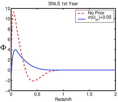
Figure 4: The weight function for the first year results of the Supernova Legacy Survey.

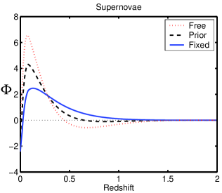
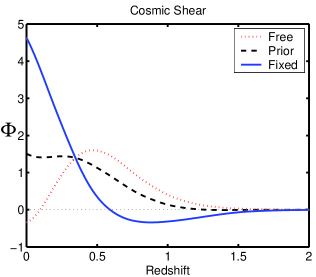
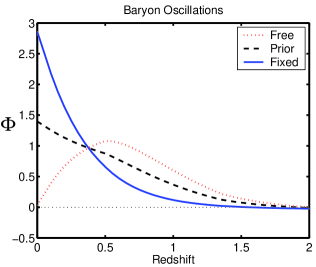
Figure 5: Here we see the influence of the $\Omega_{\rm m}$ prior. Left: Supernovae lose the region of negative weight at high redshift if $\Omega_{\rm m}$ is known correctly (solid), although it does recur at very low redshift. Center: For cosmic shear there is a significant change in redshift sensitivity when adding a stronger prior on $\Omega_{\rm m}$ (dashed and solid). Contributing information at redshift zero strengthens the influence of $w$ at low redshifts. Thus fixing the present day matter density raises the sensitivity at later times. Right: The weight function for baryon acoustic oscillations change in a similar way to cosmic shear when placing the weakest prior on $\Omega_{\rm m}$ (dotted).

We have been considering the weight functions of the potential surveys of the future, as a means to compare the techniques. However, it is also of interest to assess the meaning of present-day constraints. The weight function corresponding to the results from the first year of the Supernova Legacy Survey (SNLS) Astier et al. (2005) is shown in Fig. 4.

This data alone is insufficient to break the degeneracy between $w$ and $\Omega_{\rm m}$, as shown in Fig. 6 of Astier et al. (2005). On adding a Gaussian prior on $\Omega_{\rm m}$ of width 0.05 centered on the true value we establish a mean redshift sensitivity of 0.19.

From Fig. 6 of Astier et al. (2005) we can see that applying a prior of $\Omega_{\rm m}=0.25\pm 0.05$ would give a similar $w$ constraint to that given in their abstract from combining SNLS with baryon oscillations. Thus with this prior on $\Omega_{\rm m}$ we can already say that the average value of $w(z)$ between $0<z\lesssim 0.4$ is $\sim-1$, irrespective of its actual functional form. Conversely, we have learnt nothing of the value of $w(z)$ beyond $z\gtrsim 0.4$, despite the redshift distribution of supernovae extending out to $z=1$.

IV Influence of Priors

In the above we have, for the most part, marginalised over the cosmological and nuisance parameters with a flat prior on each, therefore assuming minimal knowledge of their values. However the shapes of the PCA eigenmodes and weight functions are expected to depend on the exact priors applied. In this section we demonstrate the variability of the weight functions by re-calculating them for different priors. Note that our previous paper Simpson and Bridle (2005) includes results for supernovae and cosmic shear where the cosmological and nuisance parameters are known exactly (delta function priors).

The tightest constraints on $w$ will arise from supplying additional datasets such as surveys of large scale structure, and the CMB. This will help break degeneracies with cosmological parameters. The most significant shift in the shape of the weight function is found to arise from applying a prior to $\Omega_{\rm m}$, and therefore we focus our discussion on this. Different priors on $\Omega_{\rm m}$ cause the weight function to shift between the forms seen in Fig. 5.

For each cosmological probe we compare

(i) “Free” (dotted line): a flat prior on $\Omega_{\rm m}$ (and flat priors on all other cosmological parameters)

(ii) “Prior” (dashed line): a Gaussian prior on $\Omega_{\rm m}$, centered on the true value, and of a width comparable to the constraint on $\Omega_{\rm m}$ placed by that particular survey. Specifically, $\sigma(\Omega_{\rm m})=0.03,0.01,0.05$ for the supernova, cosmic shear and baryon acoustic oscillations respectively. Note that if the survey areas were changed then the relative power of these $\Omega_{\rm m}$ priors would also change.

(iii) “Fixed” (solid line): a delta function prior on $\Omega_{\rm m}$ at the true value.

In all cases the weight function using a Gaussian prior lies mid-way between the two extremes. For cosmic shear and baryon oscillations, the additional information on the matter density at redshift zero naturally raises low-redshift sensitivity. Supernovae break this pattern due to the uncertainty of their absolute magnitude, which prevents us from studying the very recent behaviour of dark energy. Indeed, without calibration surveys such as the Nearby Supernova Factory Aldering et al. (2002) the uncertainty on $\mathcal{M}$ increases, and this pushes the peak to slightly higher redshift.

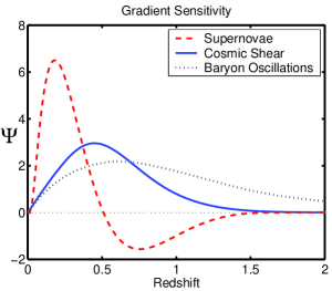
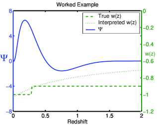
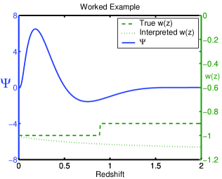
Figure 6: Left: The gradient weight function for each probe. These lines represent the sensitivity to which each technique measures the first derivative of $w$, when adopting the standard parameterisation $w=w_{0}+w_{a}(1-a)$. Center: This illustrates the interpretation of the gradient weight function, $\Psi$. The solid line shows the supernova gradient weight function; the dashed line shows the true $w(z)$ used to simulate supernova magnitudes; the dotted line shows the best fit $w(z)=w_{0}+w_{a}(1+a)$ model to the simulated data. Right: The only gradient in $w(z)$ occurs at $z\sim 1$, and since this occurs in a region of negative weight, we find that the interpreted gradient is significantly misleading.

V Higher-order Parameterisation

As data improves we are likely to advance from the single-parameter model of a constant equation of state, and look towards constraining some form of evolving equation of state. Here we shall consider the standard parameterisation $w=w_{0}+w_{a}(1-a)$ (although the results are qualitatively unchanged using the parameterisation $w=w_{0}+w_{1}z$). Adopting an analogous approach to the previous section, we define the gradient weight function

$$w_{a}^{fit}=\int\Psi(z)\frac{\mathrm{d}w}{\mathrm{d}z}(z)\mathrm{d}z.$$ (5)

The purpose of this new weight function is to quantify how much we learn about the variation of $w(z)$ from the fitted parameter values. In this section we focus on fitting $w_{a}$ to the data. The left hand panel of Fig. 6 represents the redshift sensitivity with which we observe the gradient of $w$ for each of the three probes (see Appendix A for an equivalent plot recast in terms of the sclae factor). The gradient weight function is intended to be a fairly intuitive tool. To illustrate the point of introducing $\Psi(z)$, the sensitivity to change in the equation of state, two examples are given in the centre and right hand panels of Fig. 6. In these examples we select a true equation of state in the form of a step function. The purpose of choosing this $w(z)$ is to localise all the gradient in one place, and see how the fitted value of $w_{a}$ responds. The value of the $\Psi(z)$ at the location of the step will determine our best fit.

In the central panel of Fig  6 the true $w(z)$ changes from $w=-1$ at low redshift ($z<0.4$) to $w=-0.8$ at higher redshift ($z>0.4$). Since the gradient of $w(z)$ is everywhere zero, except for a positive delta function at $z=0.4$, the resulting best-fit is readily determined from Equation 5. It is simply the magnitude of the step, multiplied by the value of $\Psi(z)$ at the location of the step.

The final plot within Fig  6 shows an example in which the step occurs where the gradient weight function is negative. As a result, the estimated gradient is a qualitatively inaccurate representation of the underlying physics.

The gradient weight function provides a quick way of predicting the fitted $w_{a}$ value for a given $w(z)$ model. Conversely, for a given $w_{a}$ obtained by some experiment, we can now interpret it using the gradient weight function. If $w_{a}$ is found to be positive then either there exists (i) a positive gradient in the true $w(z)$ in a region where the gradient weight function is positive; or (ii) a negative gradient in the true $w(z)$ in a region where the gradient weight function is negative; or some combination of the two.

Since the supernova weight function does have a negative region, this means we cannot immediately interpret a positive $w_{a}$ to imply that $w(z)$ increases with redshift. At $z>0.5$, perturbations in $\mathrm{d}w/\mathrm{d}z$ reverse the value for $w_{a}$.

Neither cosmic shear nor baryon oscillations possess significant negative weight, allowing a more straightforward interpretation of results. They are both most sensitive to changes in the true equation of state at around a redshift of 0.5, although here it is baryon oscillations which offer the highest redshift sensitivity to transitions in $w$. Mean redshift sensitivities are 0.42,0.56, 1.14 and for supernovae, cosmic shear and baryon oscillations (again, using $|\Phi(z)|$ due to the negative weight). All techniques lack sensitivity at redshift zero due to there being no physical consequence to its present value.

On combining the three probes we obtain a combined gradient weight function that resembles an average of the three separate gradient weight functions (not shown here).

We consider the gradient weight function $\Psi(z)$ to provide a more intuitive interpretation of $w_{a}$, although we could instead write $w_{a}=\int\Phi_{a}(z)w(z)dz$ as for the standard weight function (Eq. 1). We show in Appendix D that two weight functions are trivially related through

$$\Psi(z)=-\int_{0}^{z}\Phi_{a}(z^{\prime})\mathrm{d}z^{\prime}.$$ (6)

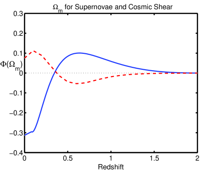
Figure 7: The $\Omega_{m}$ weight function quantifies the deviation in the fit of $\Omega_{\rm m}$ resulting from redshift variations in $w$. This plot shows that if we fit a constant $w$ when it actually increases with redshift, we will obtain an overestimated value for $\Omega_{\rm m}$ with supernovae (solid) but an underestimate with cosmic shear (dashed).

VI Mistaken matter density

So far, we discussed how the fitted values of a parameterised equation of state relate to the true function. This is of particular concern when the parametric form is a poor representation of the true equation of state. A further consequence may be the production of misleading values of the other cosmological parameters. As the most important example, we focus our attention on $\Omega_{\rm m}$.

In the work mentioned earlier, Maor et al found that fitting a constant equation of state to data simulated from $[w(z)=-0.7+0.8z,\Omega_{\rm m}=0.3]$, the best fit values were $[w_{0}=-1.75,\Omega_{\rm m}=0.65$]. Of course, this strongly erroneous value of $\Omega_{\rm m}$ could be ruled out independently. But when on a less dramatic scale this effect will persist, and becomes more difficult to exclude.

Here we quantify the apparent deviation in $\Omega_{\rm m}$ induced by fitting a constant equation of state to the data, when the true equation of state is actually evolving.

$$\Omega_{\rm m}^{\rm fit}=\Omega_{\rm m}^{\rm true}+\int\Phi_{\Omega_{\rm m}}(z)\delta w(z)\mathrm{d}z.$$ (7)

This gives the fitted value of $\Omega_{\rm m}$ in terms of the true value, and the deviation of the equation of state $\delta w(z)$ from the constant $w$ model.

The weight function $\Phi_{\Omega_{\rm m}}(z)$ is defined by this equation, but is only valid for small perturbations about the fiducial model. Other parameter’s fits may also be skewed by perturbations in $w(z)$, and the general expression for the weight function of a given parameter is outlined in Appendix E. Note that these weight functions integrate to zero, as expected since the parameter is correctly estimated if the true equation of state is a constant.

Fig. 7 compares the sensitivity with which a perturbation in $w$ will be interpreted as a change in the best-fit value of $\Omega_{\rm m}$. The responses of supernovae and cosmic shear are similar, but of opposite sign. Results from baryon oscillations are omitted as they are unable to provide competitive constraints on $\Omega_{\rm m}$, for the survey parameters considered here.

The supernova $\Omega_{\rm m}$ weight function is initially negative, becoming positive beyond $z\sim 0.4$. Consider the outcome of Eq. 7, for the case of an equation of state with positive gradient. The fitted $\Omega_{\rm m}$ value will be larger than the true value of $\Omega_{\rm m}$. This qualitatively fits the result of Maor et al. The quantitative deviation is inaccurate since such large deviations from the fiducial model leads to a major underestimation of the weight function’s amplitude at high redshift.

The cosmic shear $\Omega_{\rm m}$ weight function has the opposite shape, a good illustration of the complementarity with supernovae. So a positive gradient in $w(z)$ leads to an underestimated $\Omega_{\rm m}$ if fitting a $w={\rm const}$ model. The amplitude of the cosmic shear weight function is smaller, so this effect is slightly weaker, due to its ability to constrain $\Omega_{\rm m}$.

VII Discussion

For the foreseeable future, a full reconstruction of $w(z)$ is out of reach, but we can significantly narrow the family of functions which remain compatible with observation. We have seen how constraints from three dark energy probes, each capable of placing percent-level constraints on $w$, respond to a general $w(z)$.

The weight functions produced offer a compact and intuitive way of characterising fitted parameters such as $w_{0}$ and $w_{a}$. For a SNAP-like supernova survey sensitivity to dark energy typically peaks at $z\sim 0.05$, but this peak may be at slightly higher redshift either when applying a prior on $\Omega_{\rm m}$, or when lacking a local sample. Mean redshift sensitivities are 0.28, 0.58, and 0.54, for supernovae (SNAP-like), cosmic shear (SNAP-like), and baryon oscillations (WFMOS).

Results from baryon oscillations offer the most straightforward interpretation since their weight function is everywhere positive. This is due to a combination of factors, including the direct measure of the Hubble parameter, and the cosmological dependence of the sound horizon. At high redshift, the sensitivity is inevitably suppressed by the lack of dark energy. Indeed, at redshifts beyond those considered here, it becomes more appropriate to discuss constraints in terms of $\Omega_{\Lambda}$ as opposed to $w$.

There is a further benefit to an everywhere-positive weight function, besides a more intuitive interpretation of results. Let us consider the constraints from SNLS, where $w=-1.023\pm 0.09$. Upon adding a theoretical prior that $w(z)$ does not traverse the $-1$ boundary, the evolution of $w(z)$ becomes strongly confined, since we know the average value must be close to $-1$. This would not be the case if there were significant regions of negative weight, since higher-order terms in the Taylor expansion of $w(z)$ would enable significant evolution away from minus one, whilst maintaining a constant fit close to minus one. An alternative perspective is that the family of dark energy models constrained by a survey weight is more widely dispersed when the corresponding weight function exhibits negative regions.

The choice of dark energy probe is an eagerly anticipated one. Of primary concern is the level of reliability and accuracy of constraints which could be attained. In the case of comparable performance, one could then prioritise by considering the weight functions to indicate those which probe preferential regions. However, none of the approaches could be considered sufficiently foolproof to act alone. For example, it is unlikely that any detected deviation from $w=-1$ would become widely accepted until there is independent verification.

Appendix A The Scale Factor

Expressing our results in terms of the scale factor $a=(1+z)^{-1}$ arguably provides greater clarity, and a more physical representation of the expansion history. We define the weight function in terms of the scale factor such that

$$w_{a}^{fit}=\int\Phi(a)w(a)\mathrm{d}a.$$ (8)

This function is obtained by noting the relation $\Phi(a)\mathrm{d}a=\Phi(z)\mathrm{d}z$. The plots shown in Fig. 8 are equivalent to those in Fig. 2. Note the galaxy redshift bins for the baryon oscillations are now visible in the form of the weight function.

In an extension of this approach, Fig. 9 reproduces the gradient sensitivities to $w$, and is equivalent to the left panel of Fig. 6.

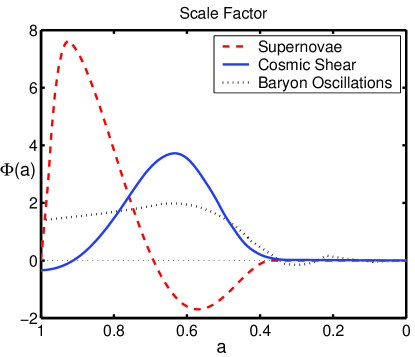
Figure 8: Here we express the sensitivity, when fitting a constant $w$, as a weighted average over the scale factor.

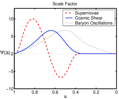
Figure 9: The sensitivity to the gradient in $w$, as a weighted average over the scale factor.

Appendix B Cosmological Dependence

Weight functions, as with PCAs, are limited by their dependence on cosmological parameters. In Fig.10, the solid line is for a fiducial model with $w=-1$ and the dashed line for a fiducial model with $w=-0.8$. We see that a change in the fiducial value of $w$ preserves the form of $\Psi$, but there is a moderate change in amplitude. If investigating a particular model, it is likely this could be compensated for by including a functional dependence of $w(z)$ on the weight function, thereby scaling the amplitude in accordance with the amount on dark energy present. For example, a scenario in which $w$ progresses towards zero (as may be anticipated to avoid fine-tuning issues) would lead to weight functions with amplified power at high redshift.

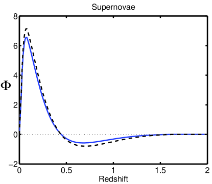
Figure 10: Here we see the enhancement of the weight function produced when the fiducial model is $w=-0.8$ (dashed line). This is pronounced at high redshift, where dark energy is now more prevalent.

Appendix C Weight Functions from PCAs

Here we derive Eq. 3 which relates the weight function for a constant $w$ fit to the principal components. The coefficients of the principal components defined in Eq. 2 provide a convenient representation of our observations:

$$\chi^{2}=\sum\Big{(}\frac{\alpha_{i}^{true}-\alpha_{i}^{fit}}{\sigma(\alpha_{i})}\Big{)}^{2}$$ (9)

and we use the orthonormality of the eigenmodes to deduce

$$\alpha^{true}_{i}=\int w(z)e_{i}(z)\mathrm{d}z\,\,\,,$$ (10)

$$\alpha^{fit}_{i}=w^{fit}\int e_{i}(z)\mathrm{d}z\,\,\,.$$ (11)

By minimising $\chi^{2}$, and solving for $w^{fit}$, the expression for $\Phi(z)$ follows from our definition of the weight function,

$$w^{fit}=\int\Phi(z)w(z)\mathrm{d}z\,\,\,,$$ (12)

$$\Phi(z)=\frac{\sum_{i}{e_{i}(z)\int e_{i}(z^{\prime})\mathrm{d}z^{\prime}/\sigma^{2}(\alpha_{i})}}{\sum_{j}(\int e_{j}(z^{\prime\prime})\mathrm{d}z^{\prime\prime})^{2}/\sigma^{2}(\alpha_{j})}\,\,.$$ (13)

In practice, we divide $z$ into 200 bins, and therefore the equivalent expression in matrix form becomes

$$\Phi(z_{j})=\frac{\sum_{i,k}K_{ij}K_{ik}}{\sum_{i,k}K_{ik}K_{ik}}$$ (14)

where we have defined

$$K_{ij}=e_{i}(z_{j})/\sigma(\alpha_{i})$$ (15)

(no summation).

Appendix D The Gradient Weight Function

We turn our attention to the derivation of the gradient weight function, which quantifies the redshift at which the derivative of $w(z)$ is measured,

$$w_{a}^{fit}=\int\Psi(z)\frac{\mathrm{d}w(z)}{\mathrm{d}z}\mathrm{d}z.$$ (16)

The most rapid evaluation of $\Psi(z)$ again involves the PCAs, and we only need consider the first few eigenmodes. We start by defining the matrix

$$K_{ij}=e_{i}(z_{j})/\sigma(\alpha_{i})$$ (17)

as this concisely represents the data in terms of observations with uncorrelated errors. When simultaneously fitting two parameters, as with $w=w_{0}+w_{a}(1-a)$, we are left with a pair of simultaneous equations, arising from the minimisation of $\chi^{2}$. Therefore

$$\Phi_{a}=\frac{(uK^{T}Ku^{T})uL^{T}K-(uK^{T}Lu^{T})uK^{T}K}{(uK^{T}Ku^{T})(uL^{T}Lu^{T})-(uK^{T}Lu^{T})^{2}}$$ (18)

where we have defined

$$L_{ij}=K_{ij}(1-1/(1+z_{j}))$$ (19)

(no summation). This is essentially an extension of Equation 19 from Saini et al. Deep Saini et al. (2003). We then convert to the gradient form $\Psi(z)$ via (6).

Appendix E The Generalised Weight Function

Previously we have considered the PCAs corresponding to measuring $w(z)$, when marginalising over other parameters. To learn of the effects of fitting other parameters, we introduce them as an extension of the principal components. Our eigenvalues are redefined as

$$\alpha^{true}_{i}=\sum_{j}e_{ij}P^{true}_{j}\,\,\,,$$ (20)

$$\alpha^{fit}_{i}=\sum_{j}e_{ij}P^{fit}_{j}\,\,\,,$$ (21)

where the components of $P$ include our original $w$ bins as before, plus the extra parameters of interest. These correspond to the $j$th component of the eigenmodes $e_{ij}$.

Thus repeating the procedure of the previous section, with $\chi^{2}$ minimisation, we arrive at a set of $n$ simultaneous equations, where $n$ is the number of fitted parameters. This is most readily solved with the division of matrices.

References

- Perlmutter et al. (1999) S. Perlmutter, G. Aldering, G. Goldhaber, R. A. Knop, P. Nugent, P. G. Castro, S. Deustua, S. Fabbro, A. Goobar, D. E. Groom, et al., Astrophys. J. 517, 565 (1999).
- Riess et al. (2004) A. G. Riess, L.-G. Strolger, J. Tonry, S. Casertano, H. C. Ferguson, B. Mobasher, P. Challis, A. V. Filippenko, S. Jha, W. Li, et al., Astrophys. J. 607, 665 (2004).
- Hoekstra et al. (2005) H. Hoekstra, Y. Mellier, L. van Waerbeke, E. Semboloni, L. Fu, M. J. Hudson, L. C. Parker, I. Tereno, and K. Benabed, First cosmic shear results from the canada-france-hawaii telescope wide synoptic legacy survey (2005), URL http://arxiv.org/abs/astro-ph/0511089.
- Cole et al. (2005) S. Cole, W. J. Percival, J. A. Peacock, P. Norberg, C. M. Baugh, C. S. Frenk, I. Baldry, J. Bland-Hawthorn, T. Bridges, R. Cannon, et al., Mon.Not.Roy.As.Soc. 362, 505 (2005).
- Lange et al. (2001) A. E. Lange, P. A. Ade, J. J. Bock, J. R. Bond, J. Borrill, A. Boscaleri, K. Coble, B. P. Crill, P. de Bernardis, P. Farese, et al., Phys. Rev. D 63, 042001 (2001).
- Spergel et al. (2003) D. N. Spergel, L. Verde, H. V. Peiris, E. Komatsu, M. R. Nolta, C. L. Bennett, M. Halpern, G. Hinshaw, N. Jarosik, A. Kogut, et al., Astrophys. J. Supp. 148, 175 (2003).
- Allen et al. (2004) S. W. Allen, R. W. Schmidt, H. Ebeling, A. C. Fabian, and L. van Speybroeck, Mon.Not.Roy.As.Soc. 353, 457 (2004).
- Riess et al. (1998) A. G. Riess, A. V. Filippenko, P. Challis, A. Clocchiatti, A. Diercks, P. M. Garnavich, R. L. Gilliland, C. J. Hogan, S. Jha, R. P. Kirshner, et al., Astron. J. 116, 1009 (1998).
- Eisenstein et al. (2005) D. J. Eisenstein, I. Zehavi, D. W. Hogg, R. Scoccimarro, M. R. Blanton, R. C. Nichol, R. Scranton, H.-J. Seo, M. Tegmark, Z. Zheng, et al., Astrophys. J. 633, 560 (2005).
- Blake and Glazebrook (2003) C. Blake and K. Glazebrook, Astrophys. J. 594, 665 (2003).
- Seo and Eisenstein (2003) H.-J. Seo and D. J. Eisenstein, Astrophys. J. 598, 720 (2003).
- Blake et al. (2004) C. A. Blake, F. B. Abdalla, S. L. Bridle, and S. Rawlings, New Astronomy Review 48, 1063 (2004).
- Linder and Huterer (2005) E. V. Linder and D. Huterer, Phys. Rev. D 72, 043509 (2005).
- Saini et al. (2004) T. D. Saini, J. Weller, and S. L. Bridle, Mon.Not.Roy.As.Soc. 348, 603 (2004).
- Huterer and Starkman (2003) D. Huterer and G. Starkman, Physical Review Letters 90, 031301 (2003).
- Knox et al. (2005) L. Knox, A. Albrecht, and Y. S. Song, in ASP Conf. Ser. 339: Observing Dark Energy (2005), pp. 107–+.
- Crittenden and Pogosian (2005) R. G. Crittenden and L. Pogosian, Investigating dark energy experiments with principal components (2005), URL http://arxiv.org/abs/astro-ph/0510293.
- Deep Saini et al. (2003) T. Deep Saini, T. Padmanabhan, and S. Bridle, Mon.Not.Roy.As.Soc. 343, 533 (2003).
- Simpson and Bridle (2005) F. Simpson and S. Bridle, Phys. Rev. D 71, 083501 (2005).
- Maor et al. (2002) I. Maor, R. Brustein, J. McMahon, and P. J. Steinhardt, Phys. Rev. D 65, 123003 (2002).
- Chevallier and Polarski (2001) M. Chevallier and D. Polarski, International Journal of Modern Physics D 10, 213 (2001).
- Linder (2003) E. V. Linder, Physical Review Letters 90, 091301 (2003).
- Linder and Huterer (2003) E. V. Linder and D. Huterer, Phys. Rev. D 67, 081303 (2003).
- Refregier et al. (2004) A. Refregier, R. Massey, J. Rhodes, R. Ellis, J. Albert, D. Bacon, G. Bernstein, T. McKay, and S. Perlmutter, Astron. J. 127, 3102 (2004).
- Glazebrook and Blake (2005) K. Glazebrook and C. Blake, Astrophys. J. 631, 1 (2005).
- Eisenstein and Hu (1998) D. J. Eisenstein and W. Hu, Astrophys. J. 496, 605 (1998).
- Blake et al. (2006) C. Blake, D. Parkinson, B. Bassett, K. Glazebrook, M. Kunz, and R. C. Nichol, Mon.Not.Roy.As.Soc. 365, 255 (2006).
- Astier et al. (2005) P. Astier, J. Guy, N. Regnault, R. Pain, E. Aubourg, D. Balam, S. Basa, R. G. Carlberg, S. Fabbro, D. Fouchez, et al., The supernova legacy survey: Measurement of , and from the first year data set (2005), URL http://arxiv.org/abs/astro-ph/0510447.
- Aldering et al. (2002) G. Aldering, G. Adam, P. Antilogus, P. Astier, R. Bacon, S. Bongard, C. Bonnaud, Y. Copin, D. Hardin, F. Henault, et al., in Survey and Other Telescope Technologies and Discoveries. Edited by Tyson, J. Anthony; Wolff, Sidney. Proceedings of the SPIE, Volume 4836, pp. 61-72 (2002). (2002), pp. 61–72.