XMM–Newton study of the complex and variable spectrum of NGC 4051

Abstract

We study the X–ray spectral variability of the Narrow Line Seyfert 1 galaxy NGC 4051 as observed during two XMM–Newton observations. To gain insight on the general behaviour, we first apply model–independent techniques such as RMS spectra and flux-flux plots. We then perform time–resolved spectral analysis by splitting the observations into 68 spectra (2 ks each). The data show evidence for a neutral and constant reflection component and for constant emission from photoionized gas, which are included in all spectral models. The nuclear emission can be modelled both in terms of a “standard model” (pivoting power law plus a black body component for the soft excess) and of a two–component one (power law plus ionized reflection from the accretion disc). Both models reproduce the source spectral variability and cannot be distinguished on a statistical ground. The distinction has thus to be made on a physical basis. The standard model results indicate that the soft excess does not follow the standard black body law (L${}_{BB}\propto T^{4}$) despite a variation in luminosity by about one order of magnitude. The resulting temperature is consistent with being constant and has the same value as observed in PG quasars. Moreover, although the spectral slope is correlated with flux, which is consistent with spectral pivoting, the hardest photon indexes are so flat ($\Gamma\sim$1.3–1.4) as to require rather unusual scenarios. Furthermore, the very low flux states exhibit an inverted $\Gamma$–flux behaviour which disagrees with a simple pivoting interpretation. These problems can be solved in terms of the two–component model in which the soft excess is not thermal, but due to the ionized reflection component. In this context, the power law has constant slope (about 2.2) and the slope–flux correlation is explained in terms of the relative contribution of the power law and reflection components which also explains the shape of the flux–flux plot relationship. The variability of the reflection component from the inner disc closely follows the predictions of the light bending model, suggesting that most of the primary nuclear emission is produced in the very innermost regions, only a few gravitational radii from the central black hole.

1 Introduction

NGC 4051 is a nearby (z=0.0023) low–luminosity Narrow–Line Seyfert 1 (NLS1) galaxy which exhibits extreme X–ray variability in flux and spectral shape on both long and short timescales. The source sometimes enters relatively long and unusual low flux states in which the hard spectrum becomes very flat ($\Gamma\sim 1$) while the soft band is dominated by a much steeper component ($\Gamma\sim 3$, or blackbody with  $kT\sim 0.12$ keV). Most remarkable is the 1998 BeppoSAX observation reported by Guainazzi et al (1998) in which the source reached its minimum historical flux state, the spectral slope was $\Gamma\simeq 0.8$, and the overall spectrum was best explained by assuming that the nuclear emission had switched off leaving only a reflection component from distant material (clearly visible in the hard spectrum) which still responded to previous higher flux levels. A different interpretation assumes that the nuclear emission in low flux states originates so close to the central black hole that only a tiny fraction can escape the gravitational pull of the hole so that the nuclear continuum is virtually undetectable at infinity (e.g. Miniutti & Fabian 2004).

In general, the 2–10 keV spectral slope appears to be well correlated with flux. However, the correlation is not linear with the slope hardening rapidly at low fluxes and reaching an asymptotic value at high fluxes (see e.g. Lamer et al 2003, based on RXTE monitoring data over about three years). This behaviour is relatively common in other sources as well, such as MCG–6-30-15, 1H 0419–577, NGC 3516 (among many others) and might be due to flux–correlated variations of the power law slope produced in a corona above an accretion disc as originally proposed by Haardt & Maraschi (1991; 1993) and Haardt et al. (1994) and related to changes in the input soft seed photons (e.g. Maraschi & Haardt 1997, Haardt, Maraschi & Ghisellini 1997, Poutanen & Fabian 1999, Zdziarski et al 2003). On the other hand, such slope–flux behaviour can be explained in terms of a two–component model (McHardy et al 1998; Shih, Iwasawa & Fabian 2002) in which a constant slope power law varies in normalisation only, while a harder component remains approximately constant hardening the spectral slope at low flux levels only, when it becomes prominent in the hard band.

In the well studied case of MCG–6-30-15, detailed spectral and variability analysis (e.g. Fabian & Vaughan 2003; Vaughan & Fabian 2004) allowed the presence of two main spectral components to be disentangled, namely a variable power law component (PLC) with constant slope, and a reflection–dominated component (RDC) from the inner accretion disc which does not follow the PLC variation, confirming for this particular case the validity of the two–component model and ruling out spectral pivoting as the main source of spectral variability. The contribution from a distant reflector is limited to 10 per cent or less (see e.g. the long Chandra observation reported by Young et al 2005) i.e. the RDC is completely dominated by lowly ionized reflection from the inner disc, including the broad relativistic Fe line. From a theoretical point of view, the lack of response of the disc RDC to the PLC variations has been interpreted in terms of strong gravitational light bending by Miniutti et al (2003) and Miniutti & Fabian (2004), which predicts this behaviour during normal flux periods and gives a correlation at low flux levels only.

It should be stressed that, in the framework of the two–component model, the 2–10 keV slope–flux correlation in NGC 4051 cannot entirely be explained by the contribution of a distant reflector in the hard band (the presence of which is required by the detection of a narrow component to the iron line). Indeed, as shown by Lamer et al (2003) the correlation is still present even if the distant reflector contribution is taken into account. Even at low flux levels, soft and hard components are significantly variable and well correlated, which excludes any dominant extended emission (torus and/or extended scattering region). Extended emission is undetected by Chandra on $\sim$ 100 pc scales (Collinge et al 2001; Uttley et al 2003). Therefore, the residual slope–flux correlation can be due to intrinsic pivoting or to an additional, almost constant, spectral component (i.e. RDC from the disc, as for MCG–6-30-15). Throughout the paper for “two–component model” we mean a parametrization of the nuclear emission in terms of two components. Other spectral components such as absorption, emission from photoionized gas, and reflection from distant matter can be present but do not represent nuclear emission.

Other important clues on the nature of the spectral variability in NGC 4051 (and other sources as well) comes from the so–called flux–flux plot analysis, first presented by Churazov, Gilfanov & Revnivtsev (2001) to demonstrate the stability of the disc emission in the high/soft state of Cyg–X1. Taylor, Uttley & McHardy (2003) have applied the same technique to a few Seyfert galaxies by using RXTE data. In the case of NGC 4051, Uttley et al (2004) have performed such an analysis by using the same XMM–Newton data we are presenting here and showed that the distribution of high, intermediate, and low flux state data points are smoothly joined together, indicating that the same process causing the spectral variability in high and intermediate flux states continues to operate even at the very low flux levels probed by the XMM–Newton data (Uttley et al 2004). This evidence seems to challenge the interpretation of the spectral variability as due to variable absorption by a substantial column of photoionized gas (Pounds et al. 2004).

Here we report results based on the two XMM–Newton observations of NGC 4051. The data have been previously analysed by Uttley et al (2004) and Pounds et al (2004) who reach different conclusions on the nature of the spectral variability in NGC 4051 and on the main spectral components that come into play. Our analysis is complementary to previous studies and offers a novel point of view that may also be relevant for other similar sources.

         

Figure 1: The broadband 0.2–10 keV XMM–Newton EPIC–pn light curves of NGC 4051 for the first (left panel, rev. 263) and the second (right panel, rev. 541) observations. The 2 ks time slices used in the time–resolved spectroscopic analysis are also shown.

2 The two XMM–Newton observations

NGC 4051 has been observed twice by XMM–Newton. The first observation took place during revolution 263 (2001 May) for $\sim$117 ks, the second during revolution 541 (2002 November) for $\sim$52 ks. These data are public and have been obtained from the XMM-Newton  data archive. The analysis has been made with the latest version of the SAS software, starting from the ODF files. During the first observation the EPIC pn and the MOS2 were operated in small window mode with the medium filter. No significant pile-up is present in the pn data, so single and double pixel events were selected. The MOS2 data show $\sim$1% of pile-up when the count rate is higher than 5 counts/s (during the first observation it sometimes reaches 15 counts/s). This could invalidate the results of time–resolved spectral variability, because, even if pile-up is not strong, its effect is increasing with flux. Thus, for the time–resolved spectral analysis, we use the MOS2 data selecting only single events and extracting the source photons within a circular region of 30^′′ radius when the count rate is lower than 5 counts/s, and within an annular region with 7^′′ and 30^′′ radii, during the higher count rate intervals. The MOS1 data were in Fast Uncompressed mode and, due to cross calibration uncertainty, we did not used those. The second observation was timed to coincide with an extended period of low X–ray emission from NGC 4051. During this observation the pile-up is negligible in all the EPIC cameras and single plus double pixel events are used for MOS1, MOS2 and pn cameras.

The background spectrum has been taken from source–free regions in the same chip as the source and ancillary and response files have been created. After filtering out periods of high background, we obtain net exposures of about 97 ks ($\sim$69 ks for the pn small window mode) and 39 ks for the first and second observation respectively. At the moment the pn camera is not well calibrated below 0.5 keV. For the data we are presenting here, for example, the ratio between the MOS and pn camera below 0.5 keV is of about 20 per cent. Thus, the data from the pn camera are used in the 0.5–10 keV band only, while MOS data are used down to 0.2 keV. All spectral fits include absorption due to the NGC 4051  line-of-sight Galactic column of $N_{H}$=1.32$\times$10²⁰ cm^-2 (Elvis et al. 1989). In the subsequent spectral analysis, errors are quoted at the 90 per cent confidence level ($\Delta\chi^{2}$=2.7 for one interesting parameter).

3 Spectral variability: a quick look

The XMM–Newton broadband light curve of NGC 4051 exhibits large amplitude count rate variations in both observations, typical for this source and for NLS1 galaxies in general. Fast large amplitude variability is superimposed on longer trends which are mainly characterized by persistent low flux periods in which variability is suppressed. The XMM–Newton light curves shown in Fig. 1 are a good representation of this behaviour which can be described in more general terms by the RMS–flux relation in which the absolute RMS variability is proportional to the source flux (Uttley & M^cHardy 2001). Light curves such as those shown in Fig. 1 are just a realization of the RMS–flux relation which naturally produces large amplitude spikes at high fluxes and periods of relative quiescence at low fluxes (e.g. Uttley, M^cHardy & Vaughan 2005).

The general shape of the broadband spectrum of NGC 4051 in both observations can be roughly described by the presence of a power law continuum, reflection from distant matter including a narrow 6.4 keV Fe line, and a prominent soft excess below about 1 keV. The Fe line is unresolved and fluxes are consistent with each other in the two observations. A Warm Absorber imprints its presence in the spectrum particularly through two edge like features at 0.74 and 0.87 keV (O VII and O VIII). Even modelling the absorption, some structures persist between 0.8 keV and 1 keV, particularly evident in the low flux state. This further structure can be interpreted as a broad absorption structure (as suggested by Pounds et al 2004), emission around 0.9 keV (see Collinge et al 2001, Uttley et al 2004), or a combination of the two.

Spectral variability is clearly present between the two observations with the source being much harder in the second, lower flux observation. Moreover, when the source is faint and hard, the spectrum above $\sim$ 2 keV appears to be more curved than in the high state. To illustrate the differences in spectral slope and hard curvature between the two observations we show the two 3–10 keV time–averaged spectra in the top panel of Fig. 2. The best–fitting power law slope is indicated, the fit including a narrow 6.4 keV Fe line as well. The spectral curvature can be interpreted as the effect of absorption by a relatively high column of ionized gas or could be the signature of a relativistically blurred reflection component from the accretion disc.

Two main mechanisms have been proposed so far to explain the spectral variability of NGC 4051. Pounds et al (2004) performed a comparative analysis of the two XMM–Newton observations based on the time–averaged spectra and on the simultaneous high–resolution RGS data in the soft band. Their main conclusions is that the spectral variability between the high flux (rev. 263) and low flux (rev. 541) observations is mainly due to variable absorption by a substantial column of photoionized gas in the line of sight. The authors suggest that in the low state (observed about 20 days after the source entered one of its characteristic low state periods) part of the gas had recombined in response to the extended period of lower X–ray flux so providing a partial coverer (with $N_{H}\sim 3.6\times 10^{23}$ cm^-2). The variable opacity of the absorber could then explain in a natural way both the flat spectrum and the hard curvature that is observed in the second low flux observation.

This interpretation is challenged by the analysis by Uttley et al (2004) who proposed spectral pivoting as the main driver of the spectral variability in NGC 4051 and pointed out that a variation in the absorber opacity in the line of sight during the low state is not consistent with the nature of the spectral variability, as revealed by flux–flux plot analysis, in which no sharp transition is seen between the two observations. The flux–flux relationship rather indicates that the spectral variability is flux–dependent and the low flux states of the first observation are virtually identical in spectral shape to the high flux state of the second. This would rule out that the low flux spectral shape during the second observation depends on the fact that data were obtained following an extended low flux state allowing the absorbing gas to recombine.

It is clear that the Pounds et al interpretation implies that the spectral shape is different in the two observations. For instance, the low flux states of the first (high flux) observation should not be as flat and curved as the spectrum in the second observation. This idea can be easily checked by comparing two spectra: the first one is representative of the very low flux state during the first observation (around 60 ks, see Fig. 1) and the second one is extracted from the second observation. We choose the two spectra to have the same exposure and approximately the same count rate. The two spectra are shown in the bottom panel of Fig. 2 in the hard band. The best fitting power law slope is also indicated. The fit also includes Fe emission at 6.4 keV. Firstly, the spectral slope is exactly the same in the two spectra. Therefore the slope is count–rate dependent and the time–averaged flat spectrum during the low flux observation has thus little to do with the extended period of low flux preceding the second observation. Secondly, the two spectra also seem to have approximately the same hard curvature. When fitted with a partial covering model, both spectra require a large column density of $\sim 0.5$–$2\times 10^{23}$ cm^-2 and a covering fraction of 60–70 per cent. This demonstrates that not only the apparent spectral slope is flux–dependent, but also that the hard curvature depends on flux only.

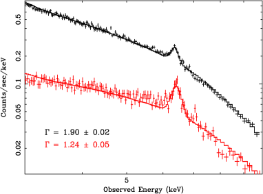
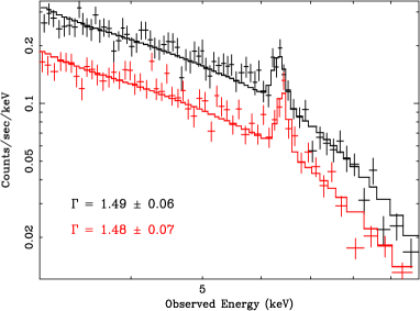
Figure 2: In the top panel we show the time averaged 3–10 keV for the first and second observation. The spectrum in the second low flux observation is flatter and much more curved that during the first high flux one. In the bottom panel we show two $\sim$ 10 ks spectra extracted from the first and second observation respectively. The one from the first observation is taken around 60 ks (see right panel of Fig. 1) and is representative of the low flux state during that (higher mean flux) observation. The two spectra are chosen from intervals that have approximately the same count rate. The two spectra have the same spectral slope and the same hard curvature showing that the spectral variability is clearly flux–dependent and that the same flat spectrum and curvature characteristic of the second observation can be found also in the first, if low flux levels are selected.

From the above analysis, it seems likely that the spectral variability in NGC 4051 is simply flux–dependent and that the second low flux observation is not peculiar but indeed identical to low flux states during the first observation. As already mentioned by Uttley et al (2004) one possible explanation for the flux–dependent spectral variability is spectral pivoting. In this paper we shall also explore an alternative explanation invoking a reflection component from the accretion disc. Before considering time–resolved spectral analysis, we perform some model–independent tests with the aim of identifying the main spectral components and their relative contribution to the spectrum and variability, in order to have a guide for our subsequent analysis.

4 RMS spectra

We start our analysis of the spectral variability of NGC 4051  by calculating the RMS spectrum, which measures the total amount of variability as a function of energy (Edelson et al. 2002; Vaughan et al. 2004; Ponti et al. 2004). Fig. 3 shows the RMS spectra during rev. 263 and 541. The RMS spectra have been calculated with time bins of $\sim$2 ks (the same as the subsequent time–resolved spectral analysis) and with energy bins chosen in order to have at least 300 counts per energy–time bin. In this way the poissonian noise is negligible compared to the RMS value and thus the use of the uncertainty given in Ponti et al. (2004) is valid.

During the high flux observation of rev. 263 (Fig. 3) the variability rapidly increases toward softer energies, i.e. the broadband emission tends to steepen as it brightens. Some reduction in the variability is seen below about 800 eV followed by a plateau below 500 eV. A similar RMS shape has been observed in other sources (Ponti et al. 2005; Vaughan et al. 2003; Vaughan et al. 2004) and the two simplest explanations for the broadband trend invoke either spectral pivoting of the variable component, or the two–component model (see e.g Markowitz, Edelson & Vaughan 2003). Another important feature of the RMS spectrum is a drop of variability at 6.4 keV, the energy of the narrow Fe line which is seen in the time–averaged spectrum. Such a drop shows that the narrow Fe line (and therefore the associated reflection continuum) is much less variable than the continuum (if variable at all) indicating an origin in distant material. Some structure is also present around 0.9 keV, with the possible presence of either a drop at that energy or two peaks.

Figure 3: The RMS spectra of the rev. 263 (top panel) and rev. 541 (bottom panel). The RMS spectra are computed with time bins of 2 ks with a minimum of 300 counts per energy bin.

In the bottom panel of the same Figure, we show the RMS spectrum obtained for the low flux observation during rev 541. The variability below 3 keV is strongly suppressed with respect to the high flux observation. Moreover, the shape of the RMS spectrum is totally different and rather unusual. The trend of increasing variability toward softer energies breaks down completely and the most striking feature is the marked drop of variability around 0.9 keV. This feature, as well as the other drop of variability at $\sim$0.55 keV, could have the same nature as the structure seen in the high flux RMS spectrum, but is much more significant and prominent here. As a sanity check, we show in Fig. 4 the source light curve around 0.9 keV and in two bands below and above for comparison. The source appears to be constant around 0.9 keV ($\chi^{2}$=144.2 for 140 degrees of freedom). The constant hypothesis is unacceptable fits in the other two bands. As in the high flux observation, the variability is also suppressed around 6.4 keV. The drop at 6–7 keV is here even more dramatic due to the reduced continuum level and therefore increased visibility of the constant narrow Fe line.

Figure 4: Source light curves during the rev. 541. The top panel shows the light curve in the big drop of variability energy band (0.86–0.93 keV, see Fig. 3); the middle panel shows the same in the 0.47–0.5 keV band; the bottom panel shows the 2.5–3.9 keV band.

4.1 Constant components

The RMS spectrum analysis given above indicate the presence of two constant or weakly variable components. The first is related to X–ray reflection and Fe emission and is seen in both observations. The second is associated with the drop in variability around 0.9 keV which is clearer in the low flux data where the contribution of the continuum is lower.

4.1.1 Reflection from distant material

Fig. 3 shows a clear minimum at 6.4 keV indicating that the narrow Fe emission line is less variable than the continuum in both observations. The Fe line is clearly detected in the time–averaged spectra of both observations. In the low flux one, the line is unresolved, has an energy of $6.42\pm 0.015$ keV, a flux of $(1.5\pm 0.2)\times$10^-5 ph s^-1 cm^-2, and an equivalent width of about 260 eV. The line energy and flux are consistent with measurements obtained in the high flux observation and also with previous data from Chandra (Collinge et al 2001) and BeppoSAX (Guainazzi et al 1998). As mentioned, a constant and narrow Fe emission line is also required by the RMS spectra. Since the Fe line must be associated with a reflection continuum, in all subsequent fits we always include a constant and neutral reflection model from Magdziarz & Zdziarski (1995) and a narrow Fe line. The reflection continuum normalization is chosen such that the Fe line equivalent width (with respect to such continuum only) is consistent with the BeppoSAX observation (EW${}_{FeK}\sim$700 eV) by Guainazzi et al (1998). This is because that observation caught NGC 4051 in a particularly low flux state in which the primary continuum had switched off leaving only reflection from distant matter in the hard band, thereby providing a most useful way to constrain that component (under the reasonable assumption that it remains constant).

4.1.2 Photo-ionized plasma emission

The second constant component is clearer in the low flux state RMS spectrum (bottom panel of Fig. 3) and appears as a deep minimum, that reach almost null variability, at around 0.9 keV and with a lower variability at $\sim$0.55 keV (see also Fig. 4). These prominent drops indicate the presence of constant emission around $\sim$0.9 and $\sim$0.5 keV, as the drop at 6.4 keV is easily interpreted as constant Fe emission. Moreover, an emission–like feature is seen in the pn spectrum of the low flux observation and in previous Chandra low flux spectra as well (Collinge et al 2001; Uttley et al 2003). The energy of the feature in the pn spectrum is $\sim$ 0.9 keV, consistent with Ne IX (and possibly Fe emission plus O VIII recombination continuum, or RRC). A second feature is also detected around 0.5–0.6 keV, where emission from O VII and O VIII is expected. As an illustration, in the top panel of Fig.5, we show the ratio of the low flux pn and MOS data to a simple continuum model comprising Galactic absorption power law and blackbody in the relevant energy band. The energies of the emission features and their intensities over the continuum correspond with the two drops seen in the RMS spectrum. The larger strength of these features during rev. 541 is due to the lower continuum. In fact, the same drop of variability at about 0.9 keV observed during the rev. 263 can be reproduced by the same constant emission lines with a higher continuum.

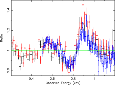
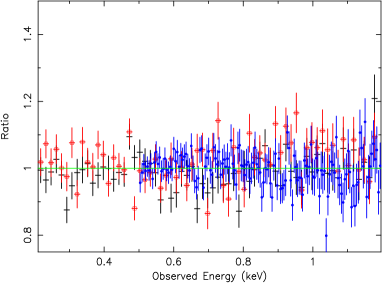
Figure 5: A portion of the MOS and pn data during the low flux observation. The top panel shows the ratio to a simple continuum model (power law plus thermal emission absorbed by the Galactic column). In the bottom panel we show the ratio to a model in which we added Oxygen lines (and edge) and emission around 0.9 keV consistently with what is seen in the high–resolution simultaneous RGS data.

To understand the nature of these constant emission components, we then inspected the simultaneous high–resolution RGS data to better search for possible narrow emission lines that could explain the features seen at CCD resolution. As already shown by Pounds et al (2004) the high–resolution RGS data during the low flux XMM–Newton observation indeed show an emission line spectrum which is very similar to that of typical Seyfert 2 galaxies (e.g.Kinkhabwala et al 2002; Bianchi et al 2005). We take the same continuum as in the CCD data and add a O VII edge at 0.74 keV to account for the absorption seen there. The most prominent emission lines are due to the O VII triplet (dominated by the forbidden and intercombination lines and with no clear resonance), the O VIII K$\alpha$ line and the N VII K$\alpha$ line (see Fig. 6). The Ne IX (forbidden) line is also clearly detected at 0.905 keV with a flux of $(3.5\pm 1.0)\times 10^{-5}$ ph s^-1 cm^-2, not enough to account for the pn feature around 0.9 keV. However, the Ne line sits on top of a broad feature most likely due to O VIII RRC and possibly unresolved Fe emission lines. When fitted with a crude Gaussian model in the RGS data, such a feature has an energy of $0.88\pm 0.01$ keV and a flux of $(5.0\pm 1.5)\times 10^{-5}$ ph s^-1 cm^-2. By combining the Ne line with this broad feature ($\sigma\simeq 20$ eV) we obtain a flux of (0.7-1.1)$\times 10^{-4}$ ph s^-1 cm^-2 around 0.9 keV.

We then included (with all parameters fixed to the RGS results) the N and O lines in the MOS/pn model, together with a O VII edge at 0.74 keV (fixed energy) and a Gaussian emission line with free energy, width, and normalization to account for the blend of Ne line plus broad feature around 0.9 keV. The resulting fit is acceptable and is shown as a ratio plot in the bottom panel of Fig. 5. As for the emission feature at 0.9 keV, we measure an energy of $0.88\pm 0.02$ keV and a flux of $(1.2\pm 0.2)\times 10^{-4}$ ph s^-1 cm^-2, consistent with the RGS upper limit. As mentioned in Pounds et al (2004) excess absorption might be present around 0.76 keV (possibly related to a M–shell unresolved transition array from Fe). If included in both CCD and RGS data, this has the effect of reducing the broad 0.9 keV feature intensity, making so much more difficult to reproduce the variability drop in the RMS spectra.

The above analysis demonstrates that emission from photoionized gas is present in the low flux data and detected both in the RGS and in the lower resolution CCD detectors. Such components, as shown by the RMS spectra, are constant over time, thus then are likely to come from relatively extended gas (see Pounds et al 2004). A constant emission component, indeed, does explain the unusual drop of variability around 0.9 keV in the low flux RMS spectrum. The line intensities are also consistent (though not detected) with the higher flux observation data. They are not detected because of the much higher continuum level. We then included, in addition to the constant neutral reflection from distant material, such lines with fixed energies and intensities (as obtained from the low flux RGS data) in all subsequent fits.

Figure 6: A portion of the RGS 1 spectrum of NGC 4051 in its low flux state. Emission by photo-ionized gas is clearly visible in the form of several emission lines. Here we show the O K$\alpha$ lines only. Such emission line spectrum is generally seen in Seyfert 2 galaxies and is detectable here thanks to the extremely low continuum.

5 Flux–flux plots: is pivoting the only solution?

Another model–independent approach that provides information on the dominant driver of the spectral variations is the flux–flux technique (see Taylor, Uttley & M^cHardy 2003; Uttley et al 2004). We recall here that a linear flux–flux relationship reveals that the data can be described by a simple two–component model where one component varies in flux but not in spectral shape, while the other remains constant both in flux and spectral shape. An offset on the hard or soft axis allows one to infer in which of the two bands the constant component contributes the most. On the other hand, if the flux–flux relationship has a power law functional form, then the data are consistent with spectral pivoting of the variable component.

Uttley et al (2004) plotted the 2–10 keV band count rate versus the 0.1–0.5 keV one and found a very accurate power law flux–flux relationship which was interpreted as evidence for spectral pivoting of the variable component. The choice of the soft and hard energy ranges by Uttley et al (2004) is driven by the requirement of having well separated bands to best reveal the spectral variability. However the 0.1–0.5 keV band does not seem to have the same variability properties of the broadband continuum. This is clearly seen in the top panel of Fig. 3 in which the soft plateau indicates the presence of a component with different variability properties than the continuum above 1 keV. Such a component is likely to be that producing the soft excess. Therefore we consider as the reference soft band the 1–1.4 keV range to avoid possible contamination from undesired components. In all previously reported analysis of the X–ray spectrum of NGC 4051, the intermediate 1–1.4 keV band is dominated by a power law continuum which is not strongly affected by absorption, soft excess, or reflection. As for the hard band, we consider the 4-10 keV range, simply to allow enough leverage for spectral variability to show up clearly.

In the top panel of Fig. 7, we show the flux–flux relationship in the chosen hard and soft bands. The two XMM–Newton observations are shown with different symbols. As already pointed out by Uttley et al (2004) the low flux state data join gently on to the normal/high flux state ones, showing that the spectral variability is likely to be due to the same mechanism at all flux levels. There is no dramatic discontinuity between the two observations suggesting, once again, that the spectral changes are not due to a dramatic change in one of the physical parameters (such a substantial change in the absorbing column, as suggested by Pounds et al 2004). The flux–flux relation is clearly non–linear with some curvature showing up especially at low fluxes. In the bottom panel, we show a binned version of the same plot (minimum of 10 points per bin). In the same figure, the solid line is the best fit for a power law model representing a situation in which the main driver of the spectral variability is spectral pivoting (see e.g. Taylor, Uttley & M^cHardy 2003 for details). The fit is performed as in Uttley et al (2004) with a power law relationship including constant components which are required in both the hard and the soft band. The power law relationship does not provide a good fit to the data ($\chi^{2}=62.4$ for 22 degrees of freedom), mainly because the model has too much curvature at high fluxes and not enough at low fluxes. This does not exclude spectral pivoting as the main driver for the spectral variability, but suggests that we need to look for an alternative explanation.

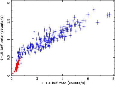
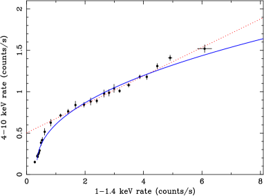
Figure 7: The flux–flux plot obtained by plotting the (pn) 4–10 keV count rate versus that in the 1–1.4 keV band. The bottom panel is just the binned version of the original flux–flux plot (top panel). The solid line is the best fit power–law relationship, while the dotted one is the best fit linear relationship if the lowest flux data points are excluded (see text for details).

In fact, if the lowest flux data points are excluded, the flux–flux relationship is linear with high accuracy. This is shown as a dotted line in the bottom panel of Fig. 7 which is the best fit linear relationship obtained when the lowest flux data points are ignored. We obtain a very good fit ($\chi^{2}=14.3$ for 15 degrees of freedom) with large hard offset of $0.50\pm 0.02$. As mentioned, a linear relationship suggests that the spectral variability is due to a two–component model, i.e. to the relative contribution of a variable component whose spectral shape is flux–independent (e.g. a constant $\Gamma$ power law varying in normalization only) and a constant or weakly variable harder component. If the flux–flux relationship at normal/high fluxes is indeed linear, one can compute the contribution of the constant component in the 4–10 keV from the y–axis offset $C_{\rm h}$. Since the mean 4-10 keV rate for the normal/high flux data points is $F_{\rm h}\simeq 1.0$, this means that the putative constant component contribution in the 4–10 keV band is as large as 50 per cent in the normal/high flux states.

However, if indeed the two–component model is a fair representation of the spectral variability at normal/high fluxes, the low flux data imply that the spectral variability must smoothly change regime at low fluxes producing the gentle low–flux bending in the relationship. Such a transition could be reproduced if, below a given flux level, the constant component (or part of it) is not constant anymore but rather follows the changes of the variable one. In fact, any two–component model in which the less variable component varies together with the variable one at low fluxes and saturates to an approximately constant flux at higher fluxes would produce the same kind of relationship as observed here.

5.1 Is the two component model consistent with the shape of the RMS spectrum?

In order to check if the source spectral variability could be due to the two–component model we try to reproduce the RMS spectrum during rev. 263 with a simple phenomenological parametrization (the RMS spectrum during rev. 541 is not considered because its shape is mainly dictated by the constant components coming from distant material). The model is composed of a direct Power–Law Component (PLC) and an ionized Reflection–Dominated Component (RDC, from Ross & Fabian 2005) the spectrum of which is convolved with a LAOR kernel with fixed inner and outer disc radius (to $1.24~{}r_{g}$ and $100~{}r_{g}$ respectively), and fixed disc inclination ($30^{\circ}$). In the RMS simulation the contribution from neutral distant reflection is also considered.

We assume that all the source variability is due to the variation of the normalisation of the direct PLC that has a spectral index fixed at $\Gamma$=2.4 (Lamer et al. 2003) and that the reflection component is completely constant not only in normalisation, but also in spectral shape (i.e. ionisation and relativistic blurring parameters). To simulate the RMS we vary the PLC normalization from the lowest to the highest value observed. For the RDC we have chosen the best fit values of the spectrum during the low flux state of rev. 263 ($\xi\simeq$50 and disc emissivity index of $\alpha\simeq$6). Figure 8 shows this simulated RMS (dotted line, green in the colour version) and, for comparison, the simulated RMS with the reflection parameters of $\xi$=5 and $\alpha$=4 (solid line, blue in the colour version), that also roughly reproduce the low flux spectrum.

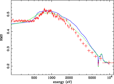
Figure 8: The observed RMS spectrum obtained during rev. 263 is compared with synthetic ones. The solid line (blue in the colour version) is obtained varying in normalization (from the lowest to the highest value observed) a PLC with $\Gamma$=2.4 and keeping a RDC with ionization parameter $\xi$=5 and disc emissivity index $\alpha$=4 completely constant. While the simulated RMS shown by the dotted line (green in colour) is calculated in the same way as above, but with $\xi\simeq$50 and $\alpha\simeq$6. In both models the contribution from neutral distant reflection is considered.

The interplay between the PLC and the RDC can roughly reproduce the shape of the RMS (within $\Delta RMS\hbox{\raise 2.15277pt\hbox{$<\lower 4.56386pt\hbox{$\kern-10.70009pt{\sim}$}$}}$0.02). This means that the two component model can explain the bulk of the spectral variability requiring no further variable component at low energy. The variability in the soft band can be explained by a variable power law and a constant soft excess (which is in this case due to constant RDC)

Clearly, a completely constant reflection component is an over–approximation. In fact, although, it is possible to reproduce the bulk of the variability, some variations of the normalization of the RDC are required in order to match with more details the RMS spectra and to reproduce the constant spectral shape below 0.5 keV (see Section 6.3.2).

6 Time–resolved spectral analysis

In sources such as NGC 4051 where large amplitude fast variability is associated with spectral variability, time–resolved or flux–resolved spectroscopy provides much more detailed information on the nature of the source than time–averaged spectroscopy. In the particular case of NGC 4051, flux–resolved spectroscopy could be a risky procedure to adopt because of the small central black hole mass (and therefore the short dynamical timescale associated with it). As an example, if we were to consider the very high flux state of the first XMM–Newton observation (see left panel of Fig. 1) and make a selection say above 40 counts/s, we would accumulate spectra from intervals sometimes spaced by 70 ks. This timescale is about 140 times the dynamical timescale at 10 $r_{g}$ (where $r_{g}=GM/c^{2}$) for a black hole mass of $\sim 5\times 10^{5}~{}M_{\odot}$ (e.g. Shemmer et al 2003) which is, in our opinion, too large a factor to extract any truly significant information on the nature of the spectral variability of the source.

We therefore explore time–resolved spectroscopy on the shortest possible timescale (set by requiring good quality time–resolved individual spectra). In the following, we present results obtained by performing such an analysis on a 2 ks timescale (about four dynamical timescales at 10 $r_{g}$). The 2 ks slices that have been used in the analysis are shown in Fig. 1 and have been numbered for reference.

6.1 The 2–10 keV $\Gamma$–flux relationship

It is well known that the 2–10 keV spectral slope in NGC 4051 (and other sources) is correlated with the source flux. In the top panel of Fig. 9, we show such a correlation when all the 2 ks spectra are fitted with a simple power–law model in the 2–10 keV band. Data for the two observations are shown with different symbols. The photon index increases with flux and seems to saturate around $\Gamma\simeq 2.2$ with a $\Delta\Gamma\simeq 1.2$ between the low and high flux states. However, the power law model is clearly inadequate to fit the 2–10 keV spectra in NGC 4051. This is because of the presence of a narrow 6.4 keV Fe K$\alpha$ line and the associated reflection continuum in the hard band. As shown above, such a component is constant and likely originates in some distant material (such as the torus).

We then fit again the 2 ks data by including the constant reflection component and show in the bottom panel of Fig. 9 the resulting $\Gamma$–flux relationship. The $\Delta\Gamma$ between the low and high flux states is now reduced to about 0.7–0.8. Again the photon index seems to saturate at high fluxes to $\Gamma\simeq 2.2$. This value is slightly different from the one ($\Gamma\simeq 2.3-2.4$) observed during a long RXTE observation campaign (Lamer et al. 2003). The difference could be due to long term spectral variability. Moreover, the photon index seems to saturate not only at high fluxes but also at low fluxes (to $\Gamma=1.3$–$1.4$). Since the two asymptotes are not extremely well defined, such behaviour could still be consistent with spectral pivoting, even though it should be stressed that the low flux photon index is still somewhat hard to be explained in terms of standard Comptonization models and would suggest some peculiar physical scenario (such as a photon–starved corona).

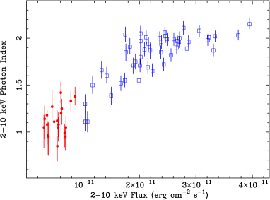
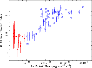
Figure 9: The best fit spectral index vs. flux in the 2–10 keV band. In the top panel the spectral model is a simple power law, while constant reflection (including a narrow Fe line) is added to the model for the bottom panel results.

On the other hand, the $\Gamma$–flux relationship seen in the bottom panel of Fig. 9 can be explained if an additional and weakly variable component is present in the 2–10 keV band. If so, such a component dominates the low flux states and the hard photon index measured there is just a measure of its intrinsic spectral shape in the 2–10 keV band, while it is overwhelmed by the power law at high fluxes where $\Gamma\simeq 2.2$ is then the intrinsic power law photon index.

In other words, as an alternative to spectral pivoting, the $\Gamma$–flux relationship can be explained by assuming the presence of i) a constant reflection component from distant matter; ii) a variable power law with constant or weakly variable slope $\Gamma\simeq 2.2$; iii) an additional component with approximate spectral shape of $\Gamma=1.3$–$1.4$ in the 2–10 keV band which must be almost constant at normal/high fluxes and is allowed to vary significantly only at low fluxes.

We point out here that our flux–flux plot analysis showed that the two–component model might indeed be appropriate in the normal/high flux states. If so, the constant component contributes by about 50 per cent in the 4–10 keV band (from the y–axis offset in the linear fit) and this is much too large a fraction to be accounted for by constant reflection from distant material (and associated narrow Fe line) which contributes in that band by only 10 per cent. The two–component model interpretation of the flux–flux relationship at normal/high fluxes implies that an additional constant component is present in the normal/high flux states and contributes by about 40 per cent to the 4–10 keV band. Such a component naturally produces the observed $\Gamma$–flux relationship because as the flux drops the spectrum becomes more and more dominated by it.

6.2 Broadband analysis I: the standard model

As a first step, we consider a simple continuum model comprising a power law plus black body (BB) emission to model the prominent soft excess. This is, in many respects, the “standard model” to fit AGN X–ray spectra and, though often crude and phenomenological, provides useful indications that can guide further analysis. The power law slope is free to vary to account for possible spectral pivoting. We add to the model neutral photoelectric absorption with column density fixed to the Galactic value. To account for the presence of absorbing ionized gas in the line of sight we include two edges (O VII and O VIII). We searched for possible variations of their energies without finding any evidence, so we fixed the absorption energies to the rest–frame ones. This is clearly a crude approximation for the effects of the warm absorber in NGC 4051, but the quality of the 2 ks spectra is not such to suggest the use of more sophisticated models. In addition, the constant components discussed above (reflection from distant matter and emission from photoionized gas) are also included in the spectral model. The overall model has six free parameters only.

The resulting fits are very good with a reduced $\chi^{2}$ ranging between 0.9 and 1.2 with a mean close to unity. Therefore, from a statistical point of view, a single model is able to describe the spectral variability of the source in a very satisfactory way. Below, we discuss the main results of the fitting procedure and their main physical consequences.

6.2.1 Variations of the central source

In Fig. 10 (top panel) we show the relation between the measured BB temperature and its intensity, which is proportional to the luminosity (in the present case A_BB=10^-4 correspond to L_BB=9.7$\times$10⁴⁰ ergs s^-1, assuming H₀=71 Mpc km^-1 s^-1). The BB luminosity spans about one order of magnitude, while the BB temperature ranges from about 90 eV to 140 eV with an average of 110–120 eV. Such a temperature is somewhat high, but can still be consistent with that expected from a black hole with mass $\simeq 5\times 10^{5}~{}M_{\odot}$ (Shemmer et al 2003; M^cHardy et al 2004) accreting at high rate (for the given black hole mass, the expected disc temperature is of the order of 70 eV for an object accreting at the Eddington rate). We point out that even in the lowest flux states the temperature (about 100 eV) is larger than predicted and, in the framework of standard disc models, would already require the system to be accreting at the Eddington rate.

If the soft excess in NGC 4051 is really due to BB emission from a constant area, we should be able to detect the BB law (L${}_{BB}\propto T^{4}$) in data spanning one order of magnitude in BB luminosity. However, such a relation is ruled out. A fit of the L_BB versus temperature data (top panel of Fig. 10) with the BB law (leaving only the normalization as a free parameter) produces a very bad fit with $\chi^{2}=1552$ for 67 degrees of freedom. The relation appears to be much steeper (with an index of 6.3–6.4 rather than 4), but even so, a power law fit is unacceptable. The measured temperature appears to be much more constant (the fit with a constant gives a $\chi^{2}=75$ for 67 degrees of freedom) than predicted by standard disc models.

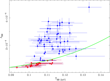
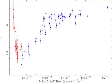
Figure 10: In the top panel we show the blackbody intensity as a function of its observed temperature. The green line shows the best fit relation between the A${}_{BB}\propto$T${}_{BB}^{4}$. In the bottom panel, we show the broadband $\Gamma$–flux relationship as obtained from the standard model fits (see text for details).

The properties of the soft excess in NGC 4051 are remarkably similar to those of 26 bright radio–quiet quasars (considered as a population) studied e.g. by Gierlinski & Done (2004) and selected from the XMM–Newton archive by their strong UV continuum (such that they have strong accretion disc emission). The quasar sample spans a wide range of black hole masses and luminosities and should therefore exhibit a wide range of disc temperatures (between a few eV to about 70 eV). However, when fitted with a cool Comptonized component, the measured temperature of the soft excess is remarkably constant throughout the sample with a mean of 120 eV (and very small variance). It is a rather surprising coincidence that this is exactly the average temperature we measure for the soft excess in NGC 4051, considering also that the black hole mass in NGC 4051 is about 3 orders of magnitude smaller than the typical black hole mass in the quasar sample. Moreover, no correlation between the measured soft excess temperature of quasars and the expected disc temperature was found, in line with the results presented above.

Such discrepancies naturally raises questions on the real nature of the X–ray soft excess. As pointed out by Gierlinski & Done (2004), the remarkable constancy of the “soft excess temperature” might indicate an origin in atomic rather than thermal physical conditions. Possible candidates seems to be absorption (e.g. from a disc wind, as suggested by Gierlinski & Done 2004) and/or ionized reflection (e.g. from the accretion disc itself, as suggested e.g. in Ross & Fabian 2005).

The “standard model” of the source emission seems to be inadequate to describe the corona parameters as well. In the bottom panel of Fig. 10 we show the power law slope as a function of the 0.5–10 keV flux. In the normal/high flux observation the photon index steepens with flux, as already pointed out in the 2–10 keV analysis. This behaviour is consistent with spectral pivoting. Once again, the lowest $\Gamma$ are of the order of 1.4 which is a hard spectral shape to be accounted for by standard Comptonization models and might require a photon–starved corona scenario. The main problems arise at very low fluxes, where the $\Gamma$–flux relation is inverted in a manner that is not consistent with simple spectral pivoting. Such behaviour could indicate the presence of an additional soft (steep) component which becomes prominent at low fluxes and is not properly accounted for by the black body component. In fact, the power law is trying to fit the soft data by steepening the index at low fluxes and leaves significant residuals in the hard band where a slope of about 1.3–1.4 would be more appropriate even at very low fluxes (see Fig. 9).

As a final comment, the mean optical depth of the ionized absorber (here modelled crudely by the O VII and O VIII edges) is of the order of 0.1–0.3, consistent with the value obtained from the RGS analysis (Pounds et al. 2004). These values are left free to vary and they seem to suggest some variations during the two observations. Nevertheless, the uncertainty associated with these is so big that a fit to the optical depth with a constant during the first observation results in a $\chi^{2}$ of 26 (O VII) and 47 (O VIII) for 47 degrees of freedom, while during the second low flux observation the $\chi^{2}$ are 29 and 7 for 19 degrees of freedom.

6.3 Broadband analysis II: the two–component model

The results of the fits with the “standard model” presented above suggest that the soft excess is not (or not completely) truly disc black body emission. Moreover, if the spectral variability is due to spectral pivoting, the power law slope at low fluxes is somewhat too hard to be accounted for by standard Comptonization (Haardt et al. 1997). In addition, a steeper component appears in the soft band at the lowest flux levels. We then explore here an alternative model to describe the spectral variability of NGC 4051.

6.3.1 Motivation: the light bending model

In order to reproduce the flux–flux plot and the $\Gamma$–flux relationship without imposing spectral pivoting, we need two main continuum components. The first one is variable in normalization only retaining an approximately constant spectral shape at all flux levels. We make here the assumption that this can be represented by a power law component (PLC). Its slope should be similar to the high–flux asymptote of the $\Gamma$–flux relationship, i.e. $\simeq$ 2.2. The other component must be almost constant in normal/high flux states where its contribution to the 4–10 keV band is of the order of 40 per cent. In the lower flux states it has instead to correlate with the PLC in order to reproduce the flux–flux plot. From the 2–10 keV $\Gamma$–flux relationship we have also some indication that its spectral shape in the hard band can be approximated by a slope of $\Gamma=$1.3–1.4.

The obvious candidate is a relativistically blurred reflection–dominated component (RDC) from a ionized accretion disc. Such a component is characterised by an X–ray spectrum which is hard in the hard band ($\Gamma=$1.3–1.6 depending on the parameters) and steep in the soft band therefore naturally producing a soft excess. As pointed out e.g. by Ross & Fabian (2005) when fitted with a thermal model in the XMM–Newton band, such a soft excess has a temperature of the order of 150 eV, very similar to the constant temperature of radio–quiet bright quasars and to the one we have measured in NGC 4051.

Since the RDC is produced in the inner disc by irradiation by the PLC, the two components should always be well correlated while, in the present case, the flux–flux plot would require that the RDC is well correlated with the PLC at low fluxes but is then only weakly variable at higher fluxes despite large changes in the PLC flux. This is however precisely the main feature of the gravitational light bending model proposed by Miniutti et al (2003) and Miniutti & Fabian (2004). In this model the variability is dominated by a power law component (PLC) which changes in flux but not in spectral shape. The PLC is (naively) assumed to have constant intrinsic luminosity and all the PLC variability is due to light bending effects as the primary PLC sources have different positions at different times with respect to the central black hole. The PLC illuminates the accretion disc giving rise to a reflection component which is affected by the relativistic effects arising in the inner disc. Such a reflection–dominated component (RDC) does not respond trivially to the PLC variability because of strong gravity effects (see Miniutti & Fabian 2004 for more details). At low fluxes the RDC is indeed well correlated with the PLC, but it gradually varies less and less as the flux increases reaching a regime in which it becomes almost constant in a range in which the PLC varies up to a factor 5. Therefore, the model successfully reproduces the two–component model (variable PLC plus constant RDC) at mean/high fluxes and since it predicts a correlation between the two components at low fluxes, it has the potential of explaining the curved flux–flux plot relationship without invoking spectral pivoting.

In this framework, low flux states correspond to situations in which the PLC originates few $r_{g}$ from the black hole strongly illuminating the innermost disc. Light bending reduces at the same time the observed PLC flux at infinity. As the PLC source is further away from the black hole, more photons can escape to infinity (so that the observed PLC flux increases) and the illuminating flux on the disc is reduced. The model therefore predicts also a relation between the emissivity profile of the RDC on the disc and flux. The lower the flux, the more centrally concentrated the disc irradiation and the steeper the emissivity.

6.3.2 Spectral fitting results and discussion

The two–component model we have tested comprises then i) a PLC with fixed slope at $\Gamma=2.2$ (consistent with the high–flux asymptote of the $\Gamma$–flux relationship) and variable normalization and ii) an ionized RDC (from Ross & Fabian 2005) the spectrum of which is convolved with a LAOR kernel with fixed inner and outer disc radius (to $1.24~{}r_{g}$ and $100~{}r_{g}$ respectively), and fixed disc inclination ($30^{\circ}$). The inner disc radius corresponds to the innermost stable circular orbit around a Kerr black hole. The only free parameters of the relativistic kernel is then the index $q$ of the disc emissivity profile ($\epsilon=r^{-q}$). The ionized reflection model is appropriate for solar abundances and has ionization parameter and normalization as free parameters, while the photon index of the illuminating power law in the RDC model is tied to that of the PLC and therefore fixed to $\Gamma=2.2$. As for the “standard model” discussed in the previous Section, the overall spectral model also includes Galactic absorption, constant emission from photoionized gas and from a distant reflector and the O VII and O VIII edges with fixed energies. The number of free parameters in the model is just the same as in the “standard model” case (6 free parameters).

The model reproduces very well the data at all flux levels with a reduced $\chi^{2}$ between 0.8 and 1.2. Given that the standard model and the two–component one have the same number of free parameters, we can directly compare the resulting averaged reduced $\chi^{2}$ which are $1.08\pm 0.07$ for the standard model and $1.06\pm 0.08$ for the two–component one. Therefore, the two–component model is statistically indistinguishable from the standard one and has to be considered as a possible alternative to be accepted or rejected on a physical rather than statistical basis.

As mentioned, the PLC used to model the data has a fixed slope of $\Gamma=2.2$ at all flux levels. In fact, we also tested a variable $\Gamma$ fit to the data and found that all 68 spectra are consistent with $\Gamma=2.2$ with only three exceptions in which the statistics is significantly better with a different power law slope (with small $\Delta\Gamma<0.15$). Therefore, we demonstrate here by direct spectral fitting that the curvature in both the flux–flux plot and the $\Gamma$–flux relationship does not imply spectral pivoting but is only consistent with it.

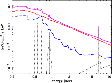
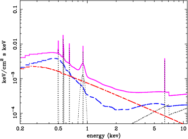
Figure 11: In the top panel we show the best fit model during the highest flux period. The PLC is shown with a dash–dotted red line; the blurred ionized reflection component is shown with a dashed blue line; the constant reflection component and the emission from photionized gas is shown with dotted grey lines and the total emission is shown with solid magenta line. In the lower panel we show the the best fit model, as before, during a low flux spectrum, showing the typical variability properties in the two–component model.

The second characteristic of the model is that the soft excess is not due to a thermal component anymore (see Fig.11). It is in fact the result of including ionized reflection from the disc, which naturally produces a soft excess. The “constant temperature” problem can then be naturally solved because of the very non–thermal nature of that component. The same kind of model successfully reproduces the soft excesses in other sources as well (e.g. Fabian et al 2004; 2005).

The ionization parameter of the reflection spectrum is not very well constrained by the data and most spectra are consistent with $\xi$ between 50 and 300 erg cm s^-1 with only few exceptions below and above (and no clear trend with flux). The reason for the non–accurate measurement of $\xi$ is probably twofold. Firstly, the spectra lack sharp emission lines which would help in constraining the ionization state (if present, the emission lines are broadened and skewed because emitted from the inner disc). Secondly, we are using a reflection model with a single uniform ionization parameter over all the disc surface from the innermost to the outermost regions. This is clearly a rough approximation for a real case in which the ionization parameter has a structured radial profile. Such approximation is likely to play a role in the non–accurate measurement of $\xi$.

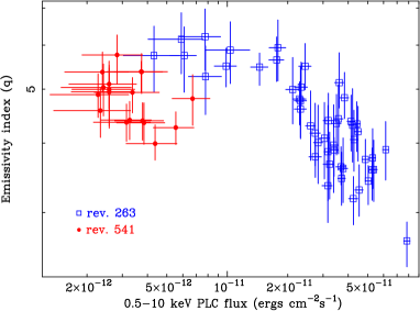
Figure 12: The emissivity index of the relativistic blurring model is plotted versus the PLC flux in the 0.5–10 keV band.

On the other hand, the disc reflection emissivity index of the relativistic blurring model is better constrained. In Fig. 12 we show the emissivity index $q$ as a function of the PLC flux. Some trend can be seen in the figure with low flux states generally corresponding to steeper emissivity profiles (with $q$ of the order of 5) than high flux ones. As mentioned above, this result is in line with the predictions of the light bending model (Miniutti & Fabian 2004).

The other main prediction of the light bending model is the RDC versus PLC relation. As mentioned, the model predicts a correlation at low flux levels and an almost constant RDC at higher flux levels, despite large variation in the PLC. In Fig. 13 we show the 0.5–10 keV flux of the RDC versus the PLC flux in the same band. The RDC is well correlated with the PLC at low flux levels (the solid line represent perfect correlation between the two components). However, as the PLC flux increases, the correlation clearly breaks down and the RDC is much less variable (about a factor 2.5) than the PLC (about a factor 7) in very good agreement with the qualitative predictions of the model. The main difference between the predicted and observed behaviour is that some residual correlation is seen at normal/high flux (while the model predicts an almost constant RDC). Such residual correlation can be easily interpreted by intrinsic luminosity variations of the PLC source which are not accounted for in the model.

We finally remark that, if the light bending interpretation is correct, the RDC versus PLC behaviour requires the primary source of PLC to be centrally concentrated above the accretion disc within 15 gravitational radii at most from the central black hole (see Miniutti & Fabian 2004). In particular, the correlation between the two component is predicted to occur only if the primary source of the PLC is within $\sim$ 5 gravitational radii from the hole. Therefore, one consequence of this interpretation is that low flux states are characterized by an extremely compact region of primary emission, well inside the relativistic region around the black hole.

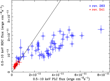
Figure 13: RDC vs. PLC 0.5–10 keV fluxes. The data clearly rule out a perfect correlation between the two components (solid line). The RDC is well correlated with the PLC at low fluxes only and varies with smaller amplitude in normal/high flux states.

7 Reproducing the RMS spectra

We tested both spectral models further by comparing the RMS spectra with synthetic ones, obtained from the best–fitting models discussed above. Obviously, the better the fits to the 2 ks spectra are, the more closely the RMS spectra will be matched, but the comparison is not trivial because the $\chi^{2}$ obtained from the time–resolved spectroscopy is a global quantity in the energy space (in fact it depend over all the energies considered) while the RMS is a local quantity (it does not depend on what is the model at other energies). It is possible, for example, that the spectral model slightly fails always in the same energy band. If this is the case, a comparison between observed and simulated RMS spectra is useful.

In Fig. 14 we show the observed and synthetic RMS spectra for both observations. In back (blue in the colour version) we plot the RMS spectra obtained from the two–component model best–fitting parameters and in grey (green) that from the standard BB plus power law model. Both models reproduce well the broadband shape of the RMS spectra in the two observations with residuals of the order of few per cent only. This is possible, allowing the three parameters of the RDC component (ionization, emissivity index and normalization) to vary (see Sect. 6.3). We do not exclude the presence of further soft component with a possibly different physical origin, but we show that that is not required when variations of the parameters of the RDC are considered. In particular, the sharp features in the RMS spectra have been reproduced thanks to the inclusion of the two constant components due to distant neutral reflection and photoionized gas emission. This reinforces our previous qualitatively interpretation indicating that the emission line intensities and their constancy (not only during each observation but also between the two one year apart) are needed in order to reproduce the RMS spectra.

The variability spectrum during the rev. 263 is less affected by the two constant components and carries more informations about the nuclear variability. Its shape can be explained equivalently well by the two models investigated. In the “standard scenario” the gradual drop of variability with energy is mainly due to the steepening of the power law slope with flux, while the lower variability at low energy is due to a less variable BB component. In the two–component model scenario it is expected that the source has lower variability both a high and low energy, because these are the regions where the almost constant relativistic reflection component is more important.

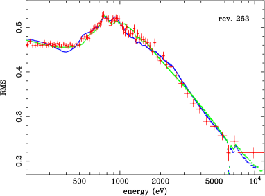
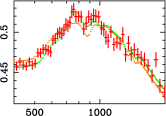
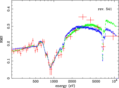
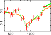
Figure 14: The observed RMS spectra of both observations are compared with synthetic ones obtained from the best–fitting standard (grey, green in the colour version) and two–component models (black, blue in colour). The inserts show the enlargement of the RMS in the soft energy band. The grey (green in the colour version) line shows the synthetic RMS obtained starting from the best–fitting parameters with the standard model and with varying optical depth edges, while the black (orange in colour) line shows the RMS expected from refitting the data with the imposition of a constant warm absorber.

In order to estimate the contribution, to the overall spectral variability, due to the variations of the warm absorber, we have simulated the RMS spectra both with constant and varying optical depth edges. The inserts of Figure 14 show the enlargement of the RMS in the soft energy band, where the effect of the warm absorber are stronger. The grey (green in the colour version) line shows the synthetic RMS obtained starting from the best–fitting parameters with the “standard model” and with varying optical depth edges, while the black (orange in the colour version) line shows the RMS expected from refitting the data with the imposition of a constant warm absorber. We show here only the results obtained considering the standard model, but similar results are obtained with the two component model. The inserts of Figure 14 show that, when the constancy of the optical depth is imposed, some deviations in the reproduction of the RMS are present. The intensity of these deviations are of the order of few percent suggesting that a variation of the warm absorber is possible but the bulk of the spectral variability is due to the interplay of the back body and power law components (power law and reflection, in the two component model) if the continuum is left completely free to vary.

8 Discussion

The analysis we presented above shows that RMS spectra, flux-flux plots and individual 2 ks spectra can be explained either in terms of a standard back body plus power law model or of a two–component model. In both cases, the presence of constant emission from photoionized gas and from a distant reflector are required.

The standard model comprises a blackbody component which provides the soft excess and a power law with variable slope (and normalization). The blackbody temperature is surprisingly constant given that its luminosity spans one order of magnitude and does not seem to follow the blackbody law ($L\propto T^{4}$). Moreover the average temperature we measure (about 110-120 eV) is remarkably similar to the average temperature measured in a sample of 26 radio–quiet quasars with typical black hole masses three orders of magnitude larger than in NGC 4051. These surprising results suggest that a pure thermal component is not appropriate to account for all the soft excess in NGC 4051. In fact, as shown in Crummy et al. (in prep.) the soft excess in type 1 active galactic nuclei is consistent, like here, with being produced by ionized reflection. The power law slope in NGC 4051  correlates with flux except at very low flux levels where the relation expected from simple spectral pivoting breaks down. Moreover the hardest photon index we measure (about 1.3–1.4) seem too hard to be explained in terms of standard Comptonization models. It should be stressed also that while spectral pivoting describes well the flux–flux plot relationship between the 0.1–0.5 keV and 2–10 keV bands (see Uttley et al 2004), it fails (or at least reduces its accuracy) when the reference soft band is chosen to be between 1 keV and 1.4 keV. This is somewhat surprising because the latter band is dominated (whatever spectral model is preferred) by the power law component, while at softer energies a contribution from the prominent soft excess is unavoidable.

In the context of the two–component model, the soft excess is instead accounted for by ionized reflection from the accretion disc which simultaneously hardens the hard spectral shape as the flux drops. The apparent constant temperature of the soft excess is then explained, because the soft excess spectral shape is dictated by atomic rather than thermal mechanisms. The two–component model is consistent with the variability being dominated by a constant–slope power law which varies in normalization only. The $\Gamma$–flux relationship is then interpreted as spurious and due to the relative flux of the power law and reflection components. The RDC is in fact correlated with the PLC at low fluxes and varies with much smaller amplitude at normal/high fluxes. Such behaviour explains not only the spurious $\Gamma$–flux relationship, but is also consistent with the flux–flux plot analysis.

9 Conclusions

We investigated the X–ray spectral variability of the Narrow Line Seyfert 1 galaxy NGC 4051  with model independent techniques (RMS spectra and Flux–Flux plots) and with time resolved spectral variability. The main features of the X–ray emission of NGC 4051 are here summarized.

1. The XMM-Newton  data of NGC 4051  show evidence for a distant neutral and constant reflection component contributing by about 10 per cent in the 4–10 keV band at mean fluxes.

2. During the low flux observation a photoionized gas imprints its presence in the soft X–ray band. This emission is consistent with being constant not only during, but also between the two observations one year apart. It is not clearly detected during the high flux observation because of a much stronger continuum.

   The constancy of this component, as well as the previous one, is primarily shown thanks to the powerful RMS spectra.

3. The nuclear emission has been interpreted both in a “standard scenario” (consisting of BB plus power law emission) and by a two–component (PLC plus ionized RDC from the disc). Both models reproduce the RMS spectra, and describe the time–resolved spectra in a comparable way from a statistical point of view. Our results are consistent with the warm absorber playing a minor role in the spectral variability.

4. The standard model results indicate that the BB emission does not follow the L${}_{BB}\propto T^{4}$ relation, even if more than an order of magnitude in luminosity is spanned. The best fit BB temperature is almost constant, clustering its value between 0.1 and 0.12 keV. The power law slope is consistent with spectral pivoting and steepens from 1.3–1.4 to about 2.2 with flux. The hardest photon indexes are so flat to require rather unusual scenarios such as a photon–starved corona. Moreover, the very low flux states exhibit an inverted $\Gamma$–flux behaviour which disagree with a simple pivoting interpretation. It is then possible that further unmodelled soft/steep component manifest itself at very low fluxes.

5. In the framework of the two–component model the soft excess is interpreted as the soft part of ionized reflection from the accretion disc. The constant temperature problem is then solved in terms of atomic rather than truly thermal processes. Moreover, the RDC explains the $\Gamma$–flux relationship at all flux levels in terms of the relative contribution of a PLC with constant slope $\Gamma=2.2$ and the RDC. The variability properties of the RDC with respect to the PLC explain also the reason why the flux–flux plot is curved without the need for invoking spectral pivoting. The RDC is well correlated with the PLC at low fluxes and varies with much smaller amplitude than it at normal/high fluxes, in line with the predictions of the light bending model in which the variability is mainly due to the fact that primary sources close to the black hole appear fainter than sources far from it because of light bending, which reduces the net observed flux at infinity as the source (of the PLC) is closer and closer to the hole.

We then propose the light bending model as a possible alternative explanation for the spectral variability of NGC 4051 in which most of the nuclear emission is emitted from the very inner regions of the flow, only few gravitational radii from the central black hole. From a physical point of view, the model does not require extreme parameters. The only true requirement is that the PLC originates in some compact region above the accretion disc and that the active region changes location in time (or disappears and a new one appears at a different location) but always within about 15 gravitational radii from the center. We stress here that if, as it is generally believed for high accretion rate sources (such as NGC 4051), the bulk of the X–ray emission comes from the inner regions of the accretion flow, the effects we are talking about are simply unavoidable. No radiation can escape from the inner regions of the flow without being affected by gravitational light bending and other relativistic effects. This is true not only for disc emission (and reflection) but also for the primary radiation.

References

- Bianchi et al (2005) Bianchi S., Miniutti G., Fabian A.C., Iwasawa K., 2005, MNRAS, 360, 380
- Collinge et al (2001) Collinge M.J. et al, 2001, ApJ, 557, 2
- Crummy et al. (2006) Crummy, J., Fabian, A. C., Gallo, L., & Ross, R. R. 2006, MNRAS, 365, 1067
- Churazov et al. (2001) Churazov, E., Gilfanov, M., & Revnivtsev, M., 2001, MNRAS, 321, 759
- Elvis et al. (1989) Elvis, M., Wilkes, B. J., & Lockman, F. J., 1989, AJ, 97, 777
- Edelson et al. (2002) Edelson, R., Turner, T. J., Pounds, K., Vaughan, S., Markowitz, A., Marshall, H., Dobbie, P., & Warwick, R., 2002, ApJ, 568, 610
- Fabian & Vaughan (2003) Fabian, A. C., & Vaughan, S., 2003, MNRAS, 340, L28
- Fabian et al. (2004) Fabian, A. C., Miniutti, G., Gallo, L., Boller, T., Tanaka, Y., Vaughan, S., & Ross, R. R., 2004, MNRAS, 353, 1071
- Fabian et al. (2005) Fabian, A. C., Miniutti, G., Iwasawa, K., & Ross, R. R., 2005, MNRAS, 361, 795
- Gierliński & Done (2004) Gierliński, M., & Done, C., 2004, MNRAS, 349, L7
- Guainazzi et al (1998) Guainazzi M. et al, 1998, MNRAS, 301, L1
- Haardt & Maraschi (1991) Haardt, F., & Maraschi, L., 1991, ApJL, 380, L51
- Haardt & Maraschi (1993) Haardt, F., & Maraschi, L., 1993, ApJ, 413, 507
- Haardt et al. (1994) Haardt, F., Maraschi, L., & Ghisellini, G., 1994, ApJL, 432, L95
- Haardt et al. (1997) Haardt, F., Maraschi, L., & Ghisellini, G., 1997, ApJ, 476, 620
- Kinkhabwala A. et al (2002) Kinkhabwala A. et al, 2002, ApJ, 575, 732
- Lamer et al (2003) Lamer G., McHardy I.M., Uttley P., Jahoda K., 2003, MNRAS, 338, 323
- Maraschi & Haardt (1997) Maraschi, L., & Haardt, F. 1997, ASP Conf. Ser. 121: IAU Colloq. 163: Accretion Phenomena and Related Outflows, 121, 101
- McHardy et al. (1998) McHardy, I. M., Papadakis, I. E., & Uttley, P., 1998, The Active X-ray Sky: Results from BeppoSAX and RXTE, 509
- McHardy et al (2004) McHardy I.M., Papadakis I.E., Uttley P., Page M.J., Mason K.O., 2004, MNRAS, 348, 783
- Magdziarz & Zdziarski (1995) Magdziarz P., Zdziarski A.A., 1995, MNRAS, 273, 837
- Markowitz, Edelson & Vaughan (2003) Markowitz A., Edelson R., Vaughan S., 2003, ApJ, 598, 935
- Miniutti et al. (2003) Miniutti, G., Fabian, A. C., Goyder, R., & Lasenby, A. N., 2003, MNRAS, 344, L22
- Miniutti & Fabian (2004) Miniutti, G., & Fabian, A. C., 2004, MNRAS, 349, 1435
- Papadakis & Lawrence (1995) Papadakis I.E., Lawrence A., 1995, MNRAS, 272, 161
- Peterson et al (1995) Peterson B.M. et al, 2000, ApJ, 542, 161
- Ponti et al. (2004) Ponti, G., Cappi, M., Dadina, M., & Malaguti, G., 2004, A&A, 417, 451
- Ponti et al. (2005) Ponti, G., Cappi, M., Dadina, Maraschi, L., Palumbo, G.G.C., Foschini, L. & Malaguti, G., 2005, Proceedings of the 6th Italian Conference on Active Galactic Nuclei, http://www.arcetri.astro.it/ agn6/
- Pounds et al (2004) Pounds K.A., Reeves J.N., King A.R., Page K.L., 2004, MNRAS, 350, 10
- Poutanen & Fabian (1999) Poutanen, J., & Fabian, A. C. 1999, MNRAS, 306, L31
- Ross & Fabian (2005) Ross, R. R., & Fabian, A. C., 2005, MNRAS, 358, 211
- Shemmer et al (2003) Shemmer O., Uttley P., Netzer H., McHardy I.M, 2003, MNRAS, 343, 1341
- Shih et al. (2002) Shih, D. C., Iwasawa, K., & Fabian, A. C., 2002, MNRAS, 333, 687
- Taylor, Uttley & McHardy (2003) Taylor R.D., Uttley P., McHardy I.M., 2003, MNRAS, 342, L31
- Uttley & McHardy (2001) Uttley P., McHardy I.M., 2001, MNRAS, 323, L26
- Uttley et al (2003) Uttley P., Fruscione A., McHardy I.M., Lamer G., 2003, ApJ, 595, 656
- Uttley et al (2004) Uttley P., Taylor R.D., McHardy I.M., Page M.J., Mason K.O., Lamer G., Fruscione A., 2004, MNRAS, 347, 1345
- Uttley, McHardy & Vaughan (2005) Uttley P., McHardy I.M., Vaughan S., 2005, MNRAS, 359, 345
- Vaughan et al. (2003) Vaughan, S., Edelson, R., Warwick, R. S., & Uttley, P., 2003, MNRAS, 345, 1271
- Vaughan & Fabian (2004) Vaughan, S., & Fabian, A. C., 2004, MNRAS, 348, 1415
- Young et al. (2005) Young, A. J., Lee, J. C., Fabian, A. C., Reynolds, C. S., Gibson, R. R., & Canizares, C. R., 2005, ArXiv Astrophysics e-prints, arXiv:astro-ph/0506082
- Zdziarski et al. (2003) Zdziarski, A. A., Lubiński, P., Gilfanov, M., & Revnivtsev, M., 2003, MNRAS, 342, 355