Voigt Profile Fitting to Quasar Absorption Lines: An Analytic Approximation to the Voigt-Hjerting Function

Abstract

The Voigt-Hjerting function is fundamental in order to correctly model the profiles of absorption lines imprinted in the spectra of bright background sources by intervening absorbing systems. In this work we present a simple analytic approximation to this function in the context of absorption line profiles of intergalactic HI absorbers. Using basic calculus tools, we derive an analytic expression for the Voigt-Hjerting function that contains only fourth order polynomial and Gaussian functions. In connection with the absorption coefficient of intergalactic neutral hydrogen, this approximation is suitable for modeling Voigt profiles with an accuracy of $10^{-4}$ or better for an arbitrary wavelength baseline, for column densities up to $\mathrm{N_{HI}}=10^{\,22}\,\mathrm{cm}^{-2}$, and for damping parameters $a\lesssim 10^{-4}$, i.e. the entire range of parameters characteristic to all Lyman transitions arising in a variety of HI absorbing systems such as Ly$\alpha$ Forest clouds, Lyman Limit systems and Damped Ly$\alpha$ systems. We hence present an approximation to the Voigt-Hjerting function that is both accurate and flexible to implement in various types of programming languages and machines, and with which Voigt profiles can be calculated in a reliable and very simple manner.

1 Introduction

Absorption processes and their signatures (absorption lines) imprinted on the spectra of bright background sources (quasars, Gamma-ray bursts, etc.) are one of the main sources of information about the physical and chemical properties of intervening systems. It is well known that information about their temperature, density, chemical abundances, and kinematics can be extracted from the analysis of these absorption lines. For instance, a detailed insight into the physical state of the intergalactic medium (IGM) is provided by the analysis of the absorption lines found in the spectra of distant quasars (QSOs) (see e.g. Hu et al., 1995; Kim et al., 1997, 2001, 2002). These lines are due mainly to absorption by neutral hydrogen (HI) present in a class of low column density absorbers generally known as Ly$\alpha$ Forest, and due to other elements in low ionisation stages (CII, CIV, SiII, MgII, FeII, OII, etc.), which arise in higher column densities absorbing systems associated with galaxies, such as the Lyman Limit Systems (LLSs) and Damped Ly$\alpha$ Absorbers (DLAs). A wealth of information about the distribution, density, temperature, metal content, etc. of these systems is now available as a result of exhaustive and extensive studies of QSO absorption lines (see e.g. Rauch, 1998; Rao, 2005, for a review on Ly$\alpha$ absorbers, and on metal systems and DLAs, respectively).

In this type of analysis, and within the realm of a given cosmological model, the number and observed central wavelength of the absorption lines provide information on the spatial distribution of the absorbing systems. Furthermore, knowledge about the actual physical state of these systems can be obtained basically from the line profiles. Both line counting and line profile measurement are tricky tasks though, since the accuracy with which they can be performed highly depends on the resolution of the observed spectra. For instance, depending on the spatial distribution of the absorbing systems, lines can appear very close to each other or even superpose (line blending), and a low spectral resolution may lead to the misidentification of the resulting composite profile as being a single, complex one. Because of this same reason, the determination of the exact shape of each individual absorption profile is far from being trivial, and misidentified profiles may lead to wrong conclusions about the properties of the absorbing systems.

If one assumes that the physical state of the absorbing medium is uniquely defined by its temperature and column density, single absorption line profiles are ideally described by Voigt profiles. Mathematically, a Voigt profile is given in terms of the convolution of a Gaussian and a Lorentzian distribution function, known as Voigt-Hjerting function (Hjerting, 1938), and a constant factor that contains information about the relevant physical properties of the absorbing medium (cf. Sect. 2.1). Any departure from a pure Voigt profile in the observed lines is expected to yield information about the kinematic properties (non-thermal broadening, rotational or turbulent macroscopic motions), as well as spatial information (clustering) of the absorbing systems.

The Voigt-Hjerting function has long been known and, consequently, various numerical methods to estimate and tabulate this function have been developed and presented (Hjerting, 1938; Harris, 1948; Finn & Mugglestone, 1965). Also, a great effort has been done in order to derive a semi-analytic approximation to this function that reproduces its behavior with high accuracy (see e.g. Whiting, 1968; Kielkopf, 1973; Monaghan, 1971), being the latter by far the one with the highest accuracy. With the help of these methods, computational subroutines have been developed that make it nowadays possible to numerically integrate this function for a wide parameter space (see e.g. Humlí$\check{\textnormal{c}}$ek, 1982).

The aim of this work is to make a further contribution to the practical handling of the Voigt-Hjerting function in order to compute Voigt profiles. Starting with an exact expression for this function in terms of Harris’ infinite series, we argue why this series may be truncated to first order in $a$ in the context of intergalactic HI absorption lines. We then show that the second term of this series can be approximated with a non-algebraic polynomial function, which is mathematically simple to handle in the sense that is does not contain singularities. Such an analytic, ’well-behaved’ expression in terms of simple functions as presented here is very attractive, since it allows one to replace the many steps and operations needed for numerical integration, or to read from look-up tables of values, by a single line with simple operations. It is also extremely flexible to implement in various types of codes and machines, and is particularly useful for computational routines in higher-level programming languages (e.g. IDL, Mathematica, Maple, etc.), in which numerical integration or look-up table reading is cumbersome, especially if absorption line profiles have to be calculated many times with moderate precision and relative high speed. For instance, such an analytic expression should be very useful to synthesise Ly$\alpha$ absorption spectra as in e.g. Zhang et al. (1997); Richter et al. (2005), or in line-fitting algorithms like AUTOVP (Davé et al., 1997) or FITLYMAN (Fontana & Ballester, 1995), used to obtain line parameters such as redshift, column density, and Doppler width from absorption Voigt profiles imprinted on observed spectra.

In the next section we briefly outline the origin of the Voigt-Hjerting function in the Physics of absorption processes, and define the context in which the desired approximation of this function is of interest to us. In Sections 3 and 4 we derive this approximation, and in Section 5 we compare the accuracy and speed of a numerical method for computing Voigt profiles based on our approximation to other existing methods. In Section 6 we present an application of our method to model Voigt profiles, and in Section 7 we summarise our main results.

2 The Voigt-Hjerting Function in the context of HI Absorption Lines

2.1 The Absorption Coefficient

The probability of a photon with an energy $E=h\,c/\lambda$ to be absorbed within a gas with column density N and kinetic temperature $T$, also known as absorption coefficient, is given by

$$\tau_{i}(\lambda)=\left(C_{i}\cdot\mathrm{N}\cdot a\right)\cdot H(a,x(\lambda))\,,$$ (1)

where

$$C_{i}\equiv\frac{4\sqrt{\pi^{3}}\,e^{2}}{m_{e}c}\frac{f_{i}}{\Gamma_{i}}$$

is a constant for the $i$th electronic transition caused by the photon absorption. Here $m_{e}$ is the electron mass, $f_{i}$ is the oscillator strength, and $\Gamma_{i}$ the damping constant or reciprocal of the mean lifetime of the transition. The function $H$ is the so-called Voigt-Hjerting function and is given by

$$H(a,x)\equiv\frac{a}{\pi}\int_{-\infty}^{+\infty}\,\frac{\mathrm{e}^{-y^{2}}}{(x-y)^{2}+a^{2}}\,\mathrm{d}y\,.$$ (2)

Let $\lambda_{i}=h\,c/E_{i}$ be the resonant wavelength of the corresponding transition , and $\Delta\lambda_{D}\equiv\frac{b}{c}\lambda_{i}$ the thermal or Doppler broadening, which defines a Doppler unit. Here, the Doppler parameter $b$ is related to the kinetic temperature of the gas via $b=\sqrt{2kT/m_{p}}$, where $k$ is the Boltzmann constant and $m_{p}$ is the proton mass. It follows from these definitions that the damping parameter

$$a\equiv\frac{\lambda_{i}^{2}\Gamma_{i}}{4\pi c\Delta\lambda_{D}}$$

quantifies the relative strength of damping broadening to thermal broadening, and that the variables $x\equiv\frac{(\lambda-\lambda_{i})}{\Delta\lambda_{D}}$ and $y\equiv\frac{\mathrm{v}}{b}$ are just the wavelength difference relative to the resonant wavelength in Doppler units, and the particle velocity in units of the Doppler parameter, respectively.

The particular form of the absorption coefficient (1) induces a characteristic absorption feature known as Voigt profile. Hence, the Voigt profile, and consequently the Voigt-Hjerting function, naturally arise in the process of absorption-line formation, when one assumes that the physical state of the absorbing medium is uniquely defined by its density and kinetic temperature. Generally speaking, it is the physical conditions what determines the shape of the absorbing features, i.e. the line profiles. Conversely, it is true that line profiles give information about the physical state of the absorbing medium. In particular, line profiles other than Voigt profiles give information about the departure of the physical conditions assumed here.

The class of HI absorbers present in the IGM (Ly$\alpha$ Forest Clouds) and associated with galaxies and larger structures (LLSs, DLAs) can be characterised by their column density $\mathrm{N_{HI}}$ and kinetic temperature, and consequently their absorption features observed on e.g. QSO spectra are well described by Voigt profiles. Their observed column densities span a range of ten orders of magnitude, approximately from $10^{12}-10^{22}\,\mathrm{cm}^{-2}$, and have temperatures that correspond to Doppler parameters approximately in the range $10-100\,\mathrm{km\,s^{-1}}$, with a median value around $b_{m}=36\,\mathrm{km\,s^{-1}}$ that decreases with redshift (Kim et al., 1997). For such a range in $b$, the damping parameter $a$ for the Lyman transitions of intergalactic HI spans a range of $9.3\cdot 10^{-9}-6.05\cdot 10^{-4}$. In this case, high values of $a$ correspond to Ly$\alpha$, while lower values are typical for higher order Lyman transitions. Transitions of other elements, such as C, Si, Mg, Fe, O, etc., and their various ionisation stages, are also typically found on QSO spectra, and their damping parameters cover a range which strongly overlaps with that of HI. This can be seen in Figure 1, where we show the distribution of $a$ for different elements (including HI) in different ionisation stages, for a Doppler parameter $b_{\mathrm{HI}}=36\,\mathrm{km\,s^{-1}}$ for HI, and assuming that the doppler parameter for other elements is related to $b_{HI}$ via $b_{X}=b_{\mathrm{HI}}\cdot\sqrt{m_{\mathrm{HI}}/m_{X}}$, where $m_{X}$ is the mass of element $X$. For clarity, we have grouped all different ionisation stages of a given element under a single label. The values of the atomic constants (central wavelength of the transition and $\Gamma$-value) have been taken from Morton (2003). The shaded area contains the values of $a$ above the range characteristic to intergalactic HI for which our approximation to the Voigt-Hjerting function–derived in the next sections–cannot be applied or should be applied with caution. Note, however, that the region spanned by $a$ for intergalactic HI, i.e. the region underneath the shaded area, contains most of the $a$-ranges spanned by all other elements, especially those corresponding to C, O, Mg, and Fe. For other elements, such as Cr or Zn, the damping parameter has values right at the upper limit of this range.

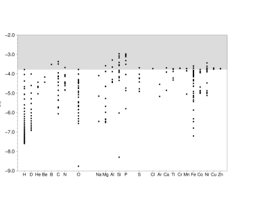
Figure 1: Value of the damping parameter $a$, assuming $b_{\mathrm{HI}}=36\,\mathrm{km\,s^{-1}}$, for different elements in different ionisation stages typically found in QSO spectra. The doppler parameter for other elements is assumed to be given by $b_{X}=b_{\mathrm{HI}}\cdot\sqrt{m_{\mathrm{HI}}/m_{X}}$ , where $m_{X}$ is the mass of element $X$. Elements are listed by increasing atomic mass on the $x$-axis, and the logarithmic value of $a$ is given on the $y$-axis. For clarity, different ionisation stages of a given element have been grouped under a single label. The shaded area marks the range above the largest value of $a$ for the intergalactic HI Lyman transitions. Note that for the sake of completeness, other elements than those found to date in QSO spectra have been included as well.

For this reason and for the sake of simplicity, in the following we will constrain our discussion to the Lyman absorption lines of intergalactic HI, but the reader shall bear in mind that the the discussion and method to synthesise Voigt profiles presented in this work can be directly applied to the transitions of other elements associated with HI absorbing systems, according to Figure 1.

2.2 The Absorption Coefficient of HI at Low Column Densities

Following Harris (1948), it is true that for $a<1$, i.e. when Doppler broadening dominates over damping broadening, the Voigt-Hjerting function (2) can be expressed as

$$H(a,x)=\sum_{n=0}^{\infty}H_{n}\,(x)\,a^{n}\,,$$ (3)

where the functions $H_{n}(x)$ are defined by

$$H_{n}\,(x)\equiv\frac{(-1)^{n}}{\sqrt{\pi}\,n!}\int_{0}^{\infty}v^{n}\mathrm{e}^{-(v/2)^{2}}\cos(xv)\,\mathrm{d}v\,.$$ (4)

These functions are bounded with respect to $n$ and $x$, and they have values of the order of unity. Indeed, taking the absolute value of the integral, neglecting the cosine, which takes values of the order of unity, and computing the resulting integral one can show that

$$|H_{n}(x)|\leq\frac{2}{\sqrt{\pi}}\approx 1.123\,,$$ (5)

for all $n\in\{0,1,2,\ldots\}$ and $x\in\mathbb{R}$. From this it follows that if $a\ll 1$, the Voigt-Hjerting function can very well be approximated to zeroth order in $a$ by the first term of the series (3), i.e. $H(a,x)\approx H_{0}(x)\,,$ as first noted by Walshaw (1955). Note that this result is exact in the limit $a\to 0$. Taking the definition (4), it follows that

$$H_{0}\,(x)\ =\,\mathrm{e}^{-x^{2}}\,,$$ (6)

and thus $H(a,x)\approx\mathrm{e}^{-x^{2}},$ for $a\ll 1$. We call this the Voigt-Hjerting function to zeroth order.

But what actually means that the condition $a\ll 1$ be satisfied, so that this zeroth order approximation can be safely used to model absorption line profiles? In order to address this, we compute for the extreme values of $a$ for intergalactic HI, $a\approx 10^{-8}$ and $a\approx 10^{-4}$, the departure of the Voigt-Hjerting function from a pure Gaussian function. This is shown in Figure 2 as the logarithmic difference between $H$ and $H_{0}$ relative to $H$ as a function of $x$, i.e. the quantity $\delta H_{0}\equiv 1-H_{0}/H$. Note how the zeroth order approximation completelly differs from the actual Voigt-Hjerting function at $x\gtrsim 3.5$ for $a=10^{-4}$, and at $x\gtrsim 4.5$ for $a=10^{-8}$. Thus, even a value of $a$ as small as $10^{-8}$ is not a sufficient condition for the zeroth order term to be a good approximation of $H$ for an arbitrary range in $x$.

Figure 2: Departure of the Voigt-Hjerting function from a pure Gaussian function for $a=10^{-8}$ (solid line) and $a=10^{-4}$ (dashed line) as a function of $x$. The departure is given as the logarithmic difference between the Voigt-Hjerting function and the zeroth order approximation in the form $\delta H_{0}\equiv 1-H_{0}/H$. The greater this quantity, the less accurate is the zeroth order approximation.

In the context of the HI absorption coefficient, the condition on $a$ for which the approximation to zeroth order of the Voigt-Hjerting function is valid, translates into a restriction on $\mathrm{N_{HI}}$, and more specifically on the quantity $C_{i}\cdot a\cdot\mathrm{N_{HI}}$. This can be seen by taking a glance at equation (1): Despite the fact that the condition $a\ll 1$ holds, the product $C_{i}\cdot a\cdot\mathrm{N_{HI}}$ can be very large for high enough column densities, and since the functions $H_{n}$ are of the order of unity, such terms can have a significant contribution to the absorption coefficient. Along this line of reasoning, and taking into consideration that the constant $C_{i}$ in equation (1) is of the order of $10^{-11}\,\mathrm{cm}^{2}$ for all Lyman transitions, it is clear that the departure of the Voigt-Hjerting function from its zeroth order approximation becomes significant in the wavelength ranges $x\gtrsim 3.5$ and $x\gtrsim 4.5$ (in Doppler units) at column densities $\mathrm{N_{HI}}\gtrsim 10^{15}\,\mathrm{cm}^{-2}$ for a damping parameter $a=10^{-4}$, and at column densities $\mathrm{N_{HI}}\gtrsim 10^{19}\,\mathrm{cm}^{-2}$ for $a=10^{-8}$. Since intervening HI absorbers typically have column densities in the range $10^{12}-10^{22}\,\mathrm{cm}^{-2}$, a Gaussian approximation to $H$ for modeling intergalactic HI absorption line profiles is only suitable for the low end of the column density range.

In addition to the factor $C_{i}\cdot a\cdot\mathrm{N_{HI}}$ being large and even more decisive for the uselessness of the zeroth order approximation for an arbitrary range in $x$, is the fact that the zeroth order term, $\mathrm{e}^{-x^{2}}$, rapidly decreases for large values of $x$ and is therefore overwhelmed by higher order terms in Harris’ expansion, which hence dominate the behavior of the absorption coefficient, as already seen in Figure 2. To shed some light on this, consider the following numerical example: Out to $x\approx 4$ (in Doppler units), and for $a=10^{-4}$, the Voigt-Hjerting function is of the order of $4.2\cdot 10^{-6}$. The zeroth order term in the series (3) satisfies $H_{0}~{}(x=4)\approx 1.1\cdot 10^{-7}$, whereas the first order term $(a\cdot H_{1})~{}(x=4)\approx 3.9\cdot 10^{-6}$. Thus, at large enough $x$, the behaviour of $\tau$ is evidently governed by the terms of order $n\geq 1$ in the series (3).

2.3 Higher Column Densities and First Order Term

Due to the arguments stated above, and even though the damping parameter satisfies $a\ll 1$, it is clear that the absorption coefficient of intergalactic HI cannot simply be approximated by a constant times $\mathrm{e}^{-x^{2}}$ for an arbitrary wavelength range and column densities grater than $10^{15}\,\mathrm{cm}^{-2}$. One actually has to take into account terms of higher order in the series (3), at least to first order in $a$, i.e. $H(a,x)\approx(H_{0}+a\cdot H_{1})~{}(x)\,.$ In fact, one should take into account all terms up to $N$th order for values of $(C_{i}\cdot a\cdot\mathrm{N_{HI}})^{-1}$ that are nearly equal or greater than the absolute difference between the sum $\sum_{n=0}^{N}H_{n}\,(x)\,a^{n}\,,$ and the exact Voigt-Hjerting function. However, as we shall show next, the approximation to first order in $a$ in Harris’ expansion is enough to model absorption line profiles with moderate to high accuracy for the range of parameters $(a,\,\mathrm{N_{HI}},\,C_{i})$ characteristic to intervening HI absorbers.

In order to prove the above statement, we look at the relative contribution of the zeroth and first order terms to the Voigt-Hjerting function for $a\in\{10^{-8},10^{-4}\}$ and an arbitrary range in $x$. This is achieved, for example, by computing the logarithm of the quantity $\delta H_{1}\equiv\left|1-(H_{0}+a\cdot H_{1})/H\right|$ as a function of $x$ for the two extreme values of $a$, as shown in Figure 3. Here we have advanced the function $H_{1}$ which is being handled in the next section. Note that the greater the contribution from the zeroth and first order term to $H$, the smaller the quantity $\delta H_{1}$. In this case, as can clearly be seen, $\delta H_{1}$ takes on values of the order of $10^{-7}$ or less over the whole wavelength range shown here and for the whole range in $a$ for intergalactic HI.

If one takes into account that $H(x)\leq 1$ for all $x$, it is obvious that the relative difference is equal or greater than the absolute difference, i.e. $\delta H_{1}\geq\left|H-(H_{0}+a\cdot H_{1})\right|$. Thus, in the case of $a\approx 10^{-4}$ and $\delta H_{1}=10^{-7}$, the departure of $H$ from its first order approximation becomes significant at column densities $\mathrm{N_{HI}}>(a\cdot\delta H_{1}\cdot C_{i})^{-1}=10^{22}\,\mathrm{cm}^{-2}$, and at even larger $\mathrm{N_{HI}}$ for $a<10^{-8}$ and/or smaller $\delta H_{1}$. Hence, the first two terms of Harris’ expansion dominate the behaviour of $H$ over the whole wavelength range shown here, with an accuracy of $10^{-7}$ or greater, for the range in $a$ characteristic to intergalactic HI. On this basis, we consider thar an approximation to first order in $a$ of the Voigt-Hjerting function in terms of the functions $H_{0}$ and $H_{1}$ is suitable to model Voigt profiles.

Figure 3: Contribution from the zeroth and first order terms of the series (3) to the absorption coefficient, when $(C_{i}\cdot a\cdot\mathrm{N_{HI}})$ is of the order of unity. The curves show the logarithmic difference between $H$ and $H_{0}+a\cdot H_{1}$, relative to $H$ as a function of $x$ for $a=10^{-8}$ (solid line) and $a=10^{-4}$ (dashed line). The smaller this difference, the greater the contribution from the zeroth and first order term to $H$. Note that the behavior of $H$ is indeed dominated with a difference of seven or more orders of magnitude by the first two terms of Harris’ expansion for the whole range in $x$ shown here. The values for $H_{1}$ were calculated according to equation (7), Section 3, using numerical integration to compute the function $F$.

Since the function $H_{0}$ is known and simple per se, we now turn to the task of finding an approximation to the function $H_{1}$ in terms of a simple, analytic expression.

3 The Dawson Function Revisited

According to definition (4) we have

$$H_{1}(x)=\frac{-4}{\sqrt{\pi}}\int_{0}^{\infty}v\,\mathrm{e}^{-v^{2}}\cos(2xv)\,\mathrm{d}v\,.$$

Integrating this equation partially, and computing the resulting Sinus transform of a Gaussian it follows (Mihalas, 1970)

$$H_{1}(x)=\frac{-2}{\sqrt{\pi}}\Big{[}1-2x\,F(x)\Big{]}\,,$$ (7)

where we adopt the notation first introduced by Miller & Gordon (1931)

$$F(x)\equiv\mathrm{e}^{-x^{2}}\int_{0}^{x}\mathrm{e}^{v^{2}}\,\mathrm{d}v\,.$$ (8)

$F$ is known as the Dawson function (Dawson, 1898).

It is evident that finding an approximation for $H_{1}$ translates into the same problem for $F$. We thus want to show that a simple analytic expression can be found which approximates the Dawson function, and hence the function $H_{1}$, accurately enough, in order for an approximation of the Voigt-Hjerting function in terms of these functions to be useful for synthesising Voigt profiles.

3.1 Properties of the Dawson Function

We briefly want to state some important properties of the Dawson-Function. First, this function is antisymmetric, i.e. $F(-x)=-F(x)$ for all $x\in\mathbb{R}$. Because of this, from now on we restrict our analysis to $x\geq 0$. Besides, it has no roots in the positive semi-axis, and $F(0)=0$, as can easily be seen from its definition (Fundamental Theorem of Calculus). Furthermore, $F$ is bounded, since $H_{1}$ is bounded itself (cf. Sect. 2.2). Indeed, differentiation with respect to $x$ gives

$$\frac{\,\mathrm{d}}{\,\mathrm{d}x}F(x)=1-2x\,F(x)\,.$$ (9)

Hence, the upper bound is given by $F(x_{0})=(2x_{0})^{-1}$, where $x_{0}$ is defined by equating $F$’s derivative to zero and solving for $x$. Actually, $F$ has its maximum at $x_{0}=0.92413$ with $F(0.92413)=0.54104$ (see e.g. Abramowitz & Stegun eds., 1965). From this last equation it follows also that equation (7) can be rewritten as

$$H_{1}(x)=\frac{-2}{\sqrt{\pi}}\frac{\,\mathrm{d}}{\,\mathrm{d}x}F(x)\,.$$ (10)

We want to know how the function $F$ behaves asymptotically, i.e. for $x\ll 1$ as well as for $x\gg 1$. Using the power series of the exponential we get

$$F(x)=\mathrm{e}^{-x^{2}}\int_{0}^{x}\sum_{n=0}^{\infty}\frac{1}{n!}v^{2n}\,\mathrm{d}v=\mathrm{e}^{-x^{2}}\cdot\sum_{n=0}^{\infty}\frac{1}{n!}\frac{x^{2n+1}}{2n+1}\,.$$ (11)

In this case, the sum and the integral operator commute, since the power series of the exponential converges uniformly in any interval $[a,b]$, particularly for $v\in[0,x]$ (see e.g. Forster, 1983). Expressing the term $\mathrm{e}^{-x^{2}}$ by its corresponding power series and rearranging terms, this last equation reads in explicit form

$$F(x)=x\cdot\Big{(}1-\frac{2}{3}x^{2}+\frac{4}{15}x^{4}+\cdots\Big{)}\,.$$

Thus, for $x\ll 1$ the Dawson function behaves asymptotically up to third order as

$$F(x)\approx x\cdot(1-\frac{2}{3}x^{2}),\qquad x\ll 1\,.$$ (12)

In order to investigate how $F$ behaves for $x\gg 1$, we first rewrite the function (8) with the replacement $v^{\prime}=x-v$ and the aid of the power series of the exponential as

$$F(x)=\sum_{n=0}^{\infty}\frac{1}{n!}I_{n}(x)\,,$$ (13)

with the definition

$$I_{n}(x)\equiv\int_{0}^{x}v^{2n}\mathrm{e}^{-2xv}\,\mathrm{d}v\,.$$ (14)

It is not hard to see that every term of the series (13) is separately bounded with respect to $x$ as well as $n$. Making the replacement $v^{\prime}=2vx$ in eq. (14), and integrating for $x\neq 0$ we get for $n\in\mathbb{N}_{0}$

$$I_{n}(x)=\frac{1}{(2x)^{2n+1}}(2n)!(1-\mathrm{e}^{-2x^{2}})-\mathrm{e}^{-2x^{2}}R_{n}(x)\,,$$ (15)

where $R_{n}(x)$ is a rather cumbersome polynomial function. Now, for $x\gg 1$, we may drop all terms which contain an exponential factor and in this way we get the asymptotic form

$$F(x)\approx\sum_{n=0}^{\infty}\frac{1}{(2x)^{2n+1}}(2n)!,\qquad x\gg 1\,.$$ (16)

It can be seen from this expression that $F$ vanishes as $(2x)^{-1}$ for $x\to\infty$, and that the first derivative (9), and thus the function $H_{1}$, also vanish in this limit as $(2x^{2})^{-1}$. From equation (9) it is also true that $F^{\prime}$ converges to unity for $x\to 0$ and that $H_{1}$ converges to $(-2\ /\sqrt{\pi})$ in this limit. Since we want our approximation to $F$, and consequently to $H_{1}$ and $H$, to be valid in the whole range $x\in[0,\infty)$, we require it to fulfill both these conditions as well.

4 The analytic approximation $D_{1}$

Equation (13), together with eq. (14), represent indeed an exact expression for the Dawson function. However, these expression are not suitable for practical computation. We therefore explore the possibility of finding an analytic expression which is easy to handle and which can be used to compute the value of $F(x)$ for $x\in[0,\infty)$. In particular, we shall see if it is possible to truncate the series (13) in order to find an approximation to $F$, which has all its properties (antisymmetry, boundedness, etc.), which converges for $x\to\infty$ as well as for $x\to 0$, and which is well defined in the whole range $[0,\infty)$. For instance, equations (12) and (16) do not fulfill these requirements. Nevertheless, they show us how our desired function has to behave asymptotically.

Let us define

$$D_{N}(x)\equiv\sum_{n=0}^{N}\frac{1}{n!}I_{n}(x)\,.$$ (17)

where the $I_{n}$’s are given by eq. (14). Using this definition we get

$$D_{1}(x)=(1-\mathrm{e}^{-2x^{2}})\cdot\left[\frac{1}{2x}+\frac{1}{4x^{3}}\right]-\mathrm{e}^{-2x^{2}}\cdot\left[\frac{x}{2}+\frac{1}{2x}\right]\,.$$ (18)

It is easy to show that this function behaves qualitatively in the same way as $F$ does, i.e. it is antisymmetric, bounded, and has no roots in the positive semi-axis. Furthermore, both these functions have the same asymptotical behavior. Indeed, up to third order we have for $x\ll 1$

$$D_{1}(x)\approx x\cdot(1-\frac{2}{3}x^{2}),\qquad x\ll 1\,.$$ (19)

as can be shown by expanding the exponentials in eq. (18) in terms of their power series. A glance at eq. (12) makes the similarity between $F$ and $D_{1}$ evident in this limit. For $x\gg 1$ we get from eq. (18), neglecting the exponentials,

$$D_{1}(x)\approx\frac{1}{2x}+\frac{1}{2^{2}x^{3}},\qquad x\gg 1\,,$$

that is the same as for $F$ (see eq. 16). Furthermore, the first derivative of $D_{1}$ with respect to $x$ is unity at $x=0$ and vanishes as $(2x^{2})^{-1}$ for $x\to\infty$. However, the maximum of $D_{1}$ is at $x=0.87269$ with $D_{1}(0.87269)=0.52212$, i.e. at slightly different values from those of $F$.

The magnitude and range of the error in approximating the Dawson function by the function $D_{1}$ can be estimated, at least qualitatively, in the following way: From equations (13) and (17) it follows that

$$F(x)=D_{1}(x)+\sum_{n=2}^{\infty}\frac{1}{n!}I_{n}(x)\,.$$ (20)

The sum in this last equation, i.e. the absolute error in our approximation $F(x)\approx D_{1}(x)$, is a positive semi-definite quantity, since each term of the sum has this property. Hence, it is true that $0\leq D_{1}(x)\leq F(x)$ for $x\in[0,\infty)$. Furthermore, since both $F$ and $D_{1}$ converge to zero for $x\to 0$ as well as for $x\to\infty$, and both these functions are bounded, it follows from eq. (20), that the error also vanishes for $x\to 0$ as well as for $x\to\infty$, that it is also bounded, and that its maximum value is less equal than ${max}\left\{F(x)-D_{1}(x)\right\}_{x>0}$. From this, and since their respective maxima are slightly shifted with respect to each other, one is led to the conclusion, that the error is constrained to a narrow range in $x$ and that the maximum error in our approximation to $F$ occurs near the maxima of these functions, i.e. in the vicinity of $x=1$.

We wont further try to quantify the actual error in our approximation to $F$. It shall be enough to know, for our purposes of finding an approximation to the Voigt-Hjerting function, that the error in the approximation $F(x)\approx D_{1}(x)$ is bounded and constrained to a narrow wavelength interval around $x=1$. Besides, we will indirectly estimate the error in this approximation when quantifying the error in our approximation to $H$ in Section 5.

4.1 The Voigt-Hjerting function to First Order

Once we have found an approximation to the Dawson function, we can use it to give the desired expression for the Voigt-Hjerting function using Harris’ expansion to first order in $a$. Replacing in equation (10) the function $F$ by our approximation $D_{1}$ (eq. 18), taking the corresponding derivative, and rearranging terms we get

$$H_{1}(x)\approx\frac{-2}{\sqrt{\pi}}K(x)\,\mathrm{e}^{-x^{2}}\,,$$ (21)

where we have defined

$$K(x)=\frac{1}{2x^{2}}\left[(4x^{2}+3)\,(x^{2}+1)\,\mathrm{e}^{-x^{2}}-\frac{1}{x^{2}}(2x^{2}+3)\sinh x^{2}\right]\,.$$ (22)

We want to highlight the fact that equation (21) is well defined, i.e. it has no singularities in the whole interval $[0,\infty)$. Furthermore, it converges to the correct value in the limits $x\to 0$ and $x\to\infty$. Indeed, it is easy to show that $\lim_{x\to 0}H_{1}(x)=\frac{-2}{\sqrt{\pi}}\,,$ and $\lim_{x\to\infty}H_{1}(x)=0\,,$ whether one uses for $H_{1}$ the exact expression (7) or the approximation (21). In contrast, in approximations to the Voigt-Hjerting function to model Voigt profiles often used in the literature (see e.g. Spitzer, 1978; Zhang et al., 1997) and given in the form $c_{1}\cdot\mathrm{e}^{-x^{2}}+c_{2}\cdot\frac{1}{x^{2}}\,,$ where the $c_{i}$’s are constants, the second term which represents the Lorentzian damping clearly diverges for $x\to 0$, and one has to artificially define the wavelength range in which this second term is used. It is customary to neglect this term for low column densities and in the vicinity of $x=0$, but how to exactly choose the radius of the vicinity is not clear and completely arbitrary. However, with an expression like equation (21) at hand, no such assumptions have to be made.

Taking into account that $a\ll 1$ in order to neglect terms of order $n\geq 2$ in the series (3), we get, using the expressions for $H_{0}$ (eq. 6) and $H_{1}$ (eq. 21), that the Voigt-Hjerting function to first order in $a$ is given by

$$H(a,x)\approx\mathrm{e}^{-x^{2}}\left[1-a\frac{2}{\sqrt{\pi}}\,K(x)\right]\,.$$ (23)

This expression is symmetric in $x$, as it should be, and thus it is valid for $x\in\mathbb{R}$ and $a\ll 1$. According to this equation, the Voigt-Hjerting function can be regarded as a ”corrected” Gaussian function, where the correction term depends on the parameter $a$. In the context of the absorption coefficient of HI, this correction term also depends on the column density $\mathrm{N_{HI}}$, of course, via the quantity $a\cdot\mathrm{N_{HI}}$.

5 Analysis

In order to quantify the quality of our approximation to $H$, we perform a test on speed as well as on precision, comparing a numerical method to compute $H$, based on our approximation, to other standard, available methods to numerically compute this function. For this purpose, we use the approach and corresponding computational routine developed by Murphy (2002), which consists of the numerical implementation in FORTRAN of four different methods to compute $H$: Harris’ $H1$ and $H2$, Humlí$\check{\textnormal{c}}$ek’s, and Monaghan’s. In Murphy’s notation, Harris’ $H1$ and $H2$ correspond to the Voigt-Hjerting function approximated by the first three and five terms of the series expansion (3), respectively. Humlí$\check{\textnormal{c}}$ek’s optimized algorithm and Monaghan’s differential approach to approximate $H$ are explained in detail in Humlí$\check{\textnormal{c}}$ek (1982) and Monaghan (1971), respectively. Our method to compute $H$ consists simply in the numerical implementation in FORTRAN of equations (22) and (23).

5.1 Speed

Following Murphy’s approach, the relative speed of all five methods are determined by calculating the time that a routine based on each method requires to compute the Voigt-Hjerting function for $x\in[0,10]$ and damping parameters $a$ in the range $10^{-8}-10^{-4}$ for a total of $1.5\cdot 10^{7}$ runs. In this way, we get that the relative speed of each method in the order $H1$ : (this work) : Humlí$\check{\textnormal{c}}$ek : $H2$ : Monaghan corresponds to 1 : 4.2 : 5.8 : 6.8 : 66.6, independent of $a$. According to this result, our method is second fastest.

5.2 Precision

Figure 4: Precision of different methods to compute the Voigt-Hjerting function, relative to Monaghan’s differential method. Shown here is the logarithmic difference as a function of $x$, i.e. the quantity $\log_{10}\,\delta H$, with $\delta H\equiv 1-H_{method}/H_{Mon}$, where $H_{Mon}$ and $H_{method}$ are, respectively, the Voigt-Hjerting function computed using Monaghan’s algorithm and each of the methods mentioned in the text: H1 (solid line), H2 (short-dashed line), Humlí$\check{\textnormal{c}}$ek (dot-dashed line), this work (long-dashed line). Each panel corresponds to a different damping parameter. Here we chose the range of $a$ characteristic to intergalactic HI, i.e. $a\in[10^{-8},10^{-4}]$. This graph was created using the approach and corresponding routine developed by Murphy (2002), and is adapted from Figure A.1 of the same work.

The precision of our method relative to the other methods mentioned above is determined in the following way: First, the values of the Voigt-Hjerting function computed using Monaghan’s algorithm for $x\in[0,10]$ and $a\in[10^{-8},10^{-4}]$ are taken as fiducial. Then, the value of $H$ for the same range in $x$ and $a$ is computed using each of these methods, and the logarithmic difference between each method and its fiducial value, i.e. the quantity $\log_{10}\,\delta H$ with $\delta H\equiv 1-H_{method}/H_{Mon}$, is calculated as a function of $x$ for each different $a$. The result is shown in Figure 4. It can be seen from this figure that Harris’ $H2$ is the second most precise method to compute $H$, if one takes Monaghan’s algorithm as fiducial, but is six times slower than Harris’ $H1$, and one-and-a-half times slower than our method, as stated in the previous section. Our method has a precision of $10^{-4}$ or better for $x\lesssim 4$. For all values of $a$, the difference peaks around $x=4$ to a value of the order of 0.01, and the precision increases again for values of $x>4$. The precision is better for smaller $a$, as expected, since the zeroth order term gains in importance in our approximation for decreasing $a$. For $a\lesssim 10^{-6}$ and $x<1.5$, our method is more precise than Harris’ $H1$ or Humlí$\check{\textnormal{c}}$ek’s, and, as seen above, 1.5 times faster than the latter.

5.3 Modeling of HI absorption profiles

We now turn to analyse how accurate is our method in order to model HI absorption profiles. Taking the whole range in column density $\log\mathrm{N_{HI}}\in[12.0,22.0]$ dex and Doppler parameters $b\in[10.0,100.0]\,\mathrm{km\,s^{-1}}$ characteristic to intergalactic HI, we synthesise for each pair $(\mathrm{N_{HI}},b)$ (with a resolution of $\Delta\log\mathrm{N_{HI}}=0.05$ dex, and $\Delta b=0.5\,\mathrm{km\,s^{-1}}$) a single Ly$\alpha$ absorption profile in the range $\lambda\in[100,2300]$ Å with a resolution of $\Delta\lambda=0.01$ Å. The absorption profile is synthesised according to equations (1) and (2), using both our method and Monaghan’s to compute $H$. We then compute for each pair $(\mathrm{N_{HI}},b)$ the absolute value of the difference between the profiles generated using these two methods relative to Monaghan’s, i.e. $\delta V\equiv|1-\mathrm{e^{-\Delta\tau}}|$, with $\Delta\tau\equiv\tau_{our}-\tau_{Mon}$, as a function of wavelength for the whole wavelength range, and pick the maximum value of this difference in the entire range. We choose to do so in order to pick up the worst cases possible, i.e. those with the lowest accuracy, and put in this way a stringent lower limit to the accuracy of our method. The result is shown as a contrast diagram on the $(\log\mathrm{N_{HI}},b)$-plane in Figure 5. Note that, in this case, it is not the logarithmic, but the linear difference which is shown. The highest precision is of the order of $10^{-16}$ or even better. However, for the sake of simplicity, any value below $10^{-4}$ has been coded as zero. The largest discrepancy between both methods, i.e. the lower limit in the precision of our method if one takes Monaghan’s as fiducial, amounts to 0.01, in agreement with the result shown in Figure 4.

Figure 5: Worst Scenario: Lower limit to the precision of our method to synthesise Voigt profiles, given as the maximum value of the difference $\delta V$ (cf. text for definition) between a Ly$\alpha$ absorption profile computed according to equation (1) using our approximation to the Voigt-Hjerting function (eq. 22 and 23) and Monaghan’s algorithm, for the whole range of values for the parameters $(\log\mathrm{N_{HI}},b)$ characteristic to intergalactic HI. The value corresponding to each pair $(\log\mathrm{N_{HI}},b)$ is the maximum value of the quantity $\delta V$ in the entire wavelength range $\lambda\in[100,2300]$ Å. For clarity, any value below $10^{-4}$ has been coded as zero.

Figure 6: Examples of Worst Scenarios: Ly$\alpha$ absorption line profile synthesised using our method (upper panel in each row) and corresponding logarithmic difference with respect to our fiducial function (lower panel in each row) for the parameter pairs $(\log\mathrm{N_{HI}},b)=(17.0,10.0)$, $(18.0,20.0)$, and $(19.0,70.0)$, from top to bottom, for which the maximum discrepancy with respect to the fiducial value of $H$ in Figure 5 is largest. The maximum difference of the order of 0.01 shown in Figure 5 amounts to an extremely narrow wavelength range between Gaussian core and Lorentzian wings. Away from these ranges, the accuracy improves significantly. For reference, and for comparison with Figure 5, a line corresponding to a constant logarithmic difference of -4 dex has been included in each of the lower panels.

As can clearly be seen, the (lower limit in the) precision of our method depends both on $b$ and $\mathrm{N_{HI}}$. While the dependence on $b$ extends to the whole range $10.0-100.0\,\mathrm{km\,s^{-1}}$, the dependence on $\mathrm{N_{HI}}$ is limited to the range $\log\mathrm{N_{HI}}=16-20$ dex. For a fixed $b$, there is a regime of values around 0.01 with a width of nearly 2 dex, which gives as a result a narrow region of low accuracy all across the plane. Along this stripe, the difference reaches its highest value of the order of 0.01 or smaller for the combinations (low $b$, low $\mathrm{N_{HI}}$) or (high $b$, high $\mathrm{N_{HI}}$), in the $b-$ and $\mathrm{N_{HI}}-$ranges stated above. Outside this stripe, the accuracy increases dramatically to values of the order of $10^{-4}$ or even better.

The origin of any inaccuracy in our method is obviously the fact that terms of order $n\geq 2$ have been neglected in the series (3), and furthermore, that the second term is this series has been approximated as well. In particular, the origin of the ’low-accuracy’ stripe on the $(\log\mathrm{N_{HI}},b)$-plane can qualitatively be understood in terms of the functional dependence of $\delta V$ on $b$ and $\mathrm{N_{HI}}$. Considering that both our method and Monaghan’s take the zeroth order term exactly into account, it is legitime to state that the quantity $\Delta H\equiv H_{our}-H_{Mon}$ has a least a dependence of first order on $a$, i.e. $\Delta H(a,x)=a\cdot h(a,x)$ where $h$ is a function that may be of zeroth order in $a$. Hence, using equation (1) and this last expression, it follows that

$$\Delta\tau(\lambda)=C^{\prime}_{i}\cdot\frac{\mathrm{N_{HI}}}{b^{2}}\cdot h(a,x)\,,\quad\mathrm{with}\quad C^{\prime}_{i}\equiv\frac{e^{2}}{4\,\sqrt{\pi}\,m_{e}\,c}\,\lambda^{2}_{i}\,f_{i}\,\Gamma_{i}\,.$$

As can be seen, $\tau$ strongly depends on the ratio $\frac{\mathrm{N_{HI}}}{b^{2}}$. Therefore, an increase in $b$ of one order of magnitude (from 10 to 100 $\mathrm{km\,s^{-1}}$) is nearly compensated (in the sense that the value of $\tau$ remains nearly constant) by an increase in $\mathrm{N_{HI}}$ of two orders of magnitude, which accounts for the stripe of 2 dex in column density seen on the $(\log\mathrm{N_{HI}},b)$-plane. Why this happens precisely between $\log\mathrm{N_{HI}}=16-20$ dex, as well as the shape of this stripe, is non-trivially related to the exact value of the constant $C^{\prime}_{i}$, the fact that $h$ may depend also on $b$ through the damping parameter $a$, and the fact that the $\Delta V$ depends effectively not on $\Delta\tau$, but on $\mathrm{e}^{-\Delta\tau}$.

It is worth mentioning that, for higher-order Lyman transitions, the precision of our method to compute Voigt profile has the same behaviour on the $(\log\mathrm{N_{HI}},b)$-plane, and is the same as or even better than the precision of the Ly$\alpha$ transition shown here. The reasons for this are, first of all, that the functional form of the absorption coefficient is obviously the same, irrespective of the transition. In addition, the lowest precision possible of 0.01 is the same for the whole range in $a$ spanned by the Lyman transitions, according to Figure 4. Furthermore, higher transitions have lower damping parameters and our approximation is better the lower $a$, as already mentioned. Finally, since the constant $C^{\prime}_{i}$ is smaller the higher the order of the transition, the critical range of lowest precision is shifted to higher column densities and higher Doppler parameters. Since the ranges in $\mathrm{N_{HI}}$ and $b$ are fixed for intergalactic HI, this has the net effect of increasing the high-precision region on the $(\log\mathrm{N_{HI}},b)$-plane–i.e. the region to the left of the stripe–for higher order transitions. In other words, the precision of our method improves from Ly$\alpha$ to higher Lyman transitions.

Even though a discrepancy of the order of 0.01 when using our method to model Voigt profiles may seem large, we want to emphasise again that this is merely an lower limit for the precision in the entire wavelength range $\lambda\in[100,2300]$ Å, in the case of Ly$\alpha$. It turns out that the range in wavelength for which the accuracy is lowest is negligible for practical purposes. In order to show this, we first choose three points on the $(\log\mathrm{N_{HI}},b)$-plane along the stripe of lowest precision, i.e. for which the maximum difference is largest. Using these parameters, we synthesise Ly$\alpha$ absorption profiles using our method and Monaghan’s, and compute again for each of these ”worst scenarios” the quantity $\delta V$ for the whole wavelength range. The result is shown in Figure 6. Each row corresponds, from top to bottom, to the parameter pairs $(\log\mathrm{N_{HI}},b)=(17.0,10.0)$, $(18.0,20.0)$, and $(19.0,70.0)$ chosen along the low-precision stripe. The upper panel of each row shows the Ly$\alpha$ absorption profile synthesised using our method, and the corresponding lower panel gives the logarithmic difference $\log_{10}\delta V$ between our method and Monaghan’s as a function of wavelength. As can be seen, the smallest discrepancies are given at the line cores, as expected, since in this regime the zeroth order term dominates and both our approach and Monaghan’s exactly take this term into account. The largest discrepancies, of the order of 0.01, are present in an extremely narrow range of $\Delta\lambda\approx 0.06$ Å for $(\log\mathrm{N_{HI}},b)=(17.0,10.0)$, of $\Delta\lambda\approx 0.17$ Å for $(\log\mathrm{N_{HI}},b)=(18.0,20.0)$, and of $\Delta\lambda\approx 0.53$ Å for $(\log\mathrm{N_{HI}},b)=(17.0,20.0)$. This discrepancies are found at the boundaries between Gaussian core and Lorentzian wings, due to the fact that our method neglects terms of order $n\geq 2$, which dominate the behaviour of $H$ in that regime. Note, however, that the difference rapidly drops with increasing distance (in Å) from the line center to values of the order of e.g. $10^{-10}$ at a distance $\Delta\lambda\approx 5$ Å for the first two rows, and $\Delta\lambda\approx 15$ Å for last row. Hence, the effective accuracy of our method is far better than 0.01 in the wavelength range shown here. For the same reason mentioned in the last paragraph, the precision for higher order Lyman transitions is of the same order as or even better than for the Ly$\alpha$ transition shown here.

6 Application

As a further test of the quality of our approximation to model Voigt profiles, and to show its accuracy in a less academic situation as in the last section, we consider fitting a synthetic spectrum to a real quasar absorption spectrum with a population of intergalactic HI absorbers spanning a representative range in $b$ and $\mathrm{N_{HI}}$ along a random line-of-sight. For this purpose we use the observed spectrum of the quasistellar source QSO J2233-606, a relatively bright ($B=17.5$) quasar at an intermediate redshift $z_{em}=2.238$.

The spectrum of the source QSO J2233-606, centered at the HDF-S, was obtained during the Commissioning of the UVES instrument at the VLT Kueyen Telescope and reduced at the Space Telescope European Coordinating Facility. The high-resolution spectroscopy (R $\approx$ 45000) was carried out with the VLT UV-Visual Echelle Spectrograph (UVES). The data were reduced in the ECHELLE/UVES context available in MIDAS. The final combined spectrum has constant pixel size of 0.05 Å and covers the wavelength range 3050-10000 Å. The S/N ratio of the final spectrum is about 50 per resolution element at 4000 Å, 90 at 5000 Å, 80 at 6000 Å, 40 at 8000 Å. The data used here are publicly available and were retrieved from www.stecf.org/hstprogrammes/J22/J22.html, in its version of November 23, 2005.

With help of the MIDAS package FITLYMAN (Fontana & Ballester, 1995), which performs line fitting through $\chi^{2}$ minimization of Voigt profiles, Cristiani & D’Odorico (2000) determined the redshifts, column densities, and Doppler widths of the identified absorption features imprinted in the spectra of QSO J2233-606. In this way, they found that the line of sight to QSO J2233-606 intersects a total of 270 Ly$\alpha$ Forest clouds, and identified other 24 absorption systems containing metal lines. The Ly$\alpha$ absorbers span a range in column density of $10^{12.20}-10^{17.10}\,\mathrm{cm^{-2}}$, and a range in Doppler parameters of $1.0-111.0\,\mathrm{km\,s^{-1}}$. The distribution of the parameter pairs $(\mathrm{N_{HI}},b)$ for these systems for $b\in[10,100]\,\mathrm{km\,s^{-1}}$ is shown in Figure 7.

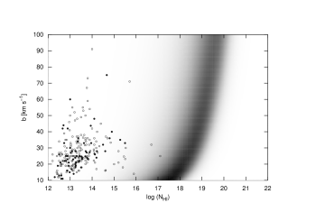
Figure 7: Distribution in column density and Doppler parameter of the absorbing systems along the line-of-sight towards the source QSO J2233-606. This particular LOS contains a total of 264 absorbing systems with $b\in[10,100]\,\mathrm{km\,s^{-1}}$ in the range $3050-10000$ Å (open circles), 69 from which are in the wavelength range $3340-3530$ Å (filled circles). The data was taken from Cristiani & D’Odorico (2000). For reference and comparison, the contrast diagram shown in Figure 5 has also been included.

Using this list of Ly$\alpha$ line parameters $(z_{abs},\ b,\ \mathrm{N_{HI}})$, we generate a synthetic spectrum of the QSO J2233-606 in the wavelength range $3340-3530$ Å with a higher resolution than that of the observed spectrum of $\Delta\,\lambda=0.01$ Å, using eqs. (1), (21), (22), and (23). We synthesise a second spectrum using Monaghan’s algorithm, and compute the logarithmic difference $\delta V$ between these two synthetic spectra in the same fashion as in the previous section. In this way, we test again our method against the highest-precision method available, for a typical range in column densities and Doppler parameters present in a QSO spectrum. The result is shown in Figure 8. The upper panels of each row show the observed spectrum and the spectrum synthesised using our method, whereas the lower panels show the logarithmic difference between both synthetic spectra. We choose to cut off the logarithmic difference at $10^{-16}$, since differences smaller than these are out of the range of the highest available numerical precision. It can be seen again, as in Figure 6, that the smallest discrepancies are given at the line cores, and the largest, of the order of $10^{-4}$, are given at the wings (cf. discussion of Figure 6, Section 5.3). As can be seen from the column density and Doppler parameter distribution in Figure 7, the largest discrepancies in this wavelength range are consistent with the maximum absolute differences shown in Figure 5. Note that in the spectral regions where no apparent absorption features are found, the logarithmic difference does not fall to $-\infty$, as one would naively expect. These features are present in Figure 6 as well. The reason for this ’valley-shaped’ features is that, even though having small values away from the line center, the function $H$ does not fall to zero, and thus in these regions the wings of two or more lines overlap. Strictly speaking, in these regions there is always some absorption left, i.e. $\tau<1$, and different methods to compute $H$ will account for this effect differently. Again, since our method neglects terms of order $n\geq 2$, the absorption in these regimes differs from its fiducial value. The lack of this terms in our approximation to $H$ is also pointed out pictorially by the local maxima symmetrically placed around the deeps corresponding to the logarithmic difference at the line cores.

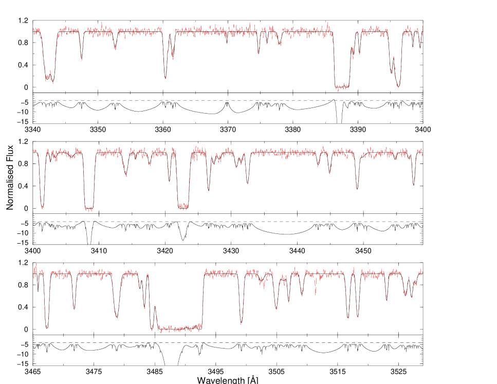
Figure 8: Observed (dashed line) and synthetic (solid line) spectrum of the quasar HDF-S QSO J2233-606 (upper panel in each row) in the wavelength range $[3340,3530]$ Å (cf. text for reference). The synthetic spectrum was generated using our approximation to the Voigt-Hjerting function and the list of line parameters obtained by Cristiani & D’Odorico (2000). The lower panels show the logarithmic difference between our synthetic spectrum and one generated using the same list of line parameters and Monaghan’s algorithm to calculate Voigt profiles. For reference, we include in the difference panels an horizontal line corresponding to a logarithmic difference of -4 dex.

7 Summary

The absorption lines imprinted in the spectra of background sources yield a wealth of information about the physical and chemical properties of the intervening absorbing material, as is the case of intervening neutral hydrogen (HI) systems embedded in the intergalactic medium (IGM) and associated with galaxies and larger structures. In order to extract the desired information from these absorption lines, their profiles have to be modeled in a proper way. In the case of absorption features found on QSO spectra, absorption line profiles are best modeled by Voigt profiles, which are mathematically given in terms of the Voigt-Hjerting function.

In this work, we presented a simple analytic approximation to the Voigt-Hjerting function with which Voigt profiles can be modeled for an arbitrary range in wavelength (or frequency), column densities up to $10^{22}\ \mathrm{cm}^{-2}$, and for damping parameters satisfying $a\lesssim 10^{-4}$. Starting with an exact expression for the Voigt-Hjerting function in terms of Harris’ expansion that is valid for $a<1$, we showed that the zeroth order term of this series, a Gaussian function, is suitable for modeling absorption line profiles emerging in a medium with low column density $\mathrm{N_{HI}}\lesssim 10^{15}\mathrm{cm}^{-2}$. However, for higher column densities, terms of higher order have to be taken into account. A key point leading to this conclusion is the fact that it is not the damping parameter alone, but rather the factor $a\cdot\mathrm{N_{HI}}$ that determines to which extent terms of order higher than zeroth in Harris’ expansion may or may not be neglected. We showed that the departure of the actual Voigt-Hjerting function from the first two terms in Harris’ expansion is of the order of $10^{-7}$ or less for an arbitrary wavelength range and $a\lesssim 10^{-4}$. Hence, we concluded that with an approximation to first order in $a$ to the Voigt-Hjerting function Voigt profiles can be modeled with moderate to high accuracy.

On this basis, we obtained a simple analytic expression for the Voigt-Hjerting function and consequently for the absorption coefficient of intergalactic HI, in terms of an approximation for the second term $H_{1}$ of Harris’ expansion. The main advantages of the analytic expression we presented here are, first, that it is valid for an arbitrary wavelength range, in the sense that is has no singularities. In addition, it is simple and flexible to implement in a variety of programming languages to numerically compute Voigt profiles with moderate speed and moderate to high accuracy. As a matter of fact, our method to compute the Voigt-Hjerting function is faster with respect to other known standard methods, for instance, Humlí$\check{\textnormal{c}}$ek’s or Monaghan’s algorithm. Furthermore, our approximation reaches an accuracy of $10^{-4}$ or better in a wide wavelength range, and of the order of than $10^{-2}$ only a negligible wavelength interval, for values of $a$ and $\mathrm{N_{HI}}$ characteristic to intergalactic HI absorbers. Our method thus offers a great compromise between speed, accuracy, and flexibility in its implementation.

Even though we did not extend our discussion in this work to other transitions typically present in quasar absorption spectra and associated to HI absorbers, such as metal lines, our method to synthesise Voigt profiles can certainly be applied to most of these elements as well, since their column densities are obviously the same, and their ranges in $a$ strongly overlap with the range of $a$ for intergalactic HI, for which our approximation to the Voigt-Hjerting function is valid. As a matter of fact, our approximation is valid to model absorption Voigt profiles found in any type of spectrum (stellar, solar, etc.), which arise in a medium whose damping parameter and column density satisfy $a\lesssim 10^{-4}$ and $\mathrm{N_{HI}}\leq 10^{22}\,\mathrm{cm}^{-2}$, respectively.

References

- Abramowitz & Stegun eds. (1965) Abramowitz, M. & Stegun, I.A., eds. 1965, Handbook of Mathematical Functions National Bureau of Standards
- Cristiani & D’Odorico (2000) Cristiani, S., & D’Odorico, V. 2000, AJ, 120, 1648
- Davé et al. (1997) Davé, R., Hernquist, L., Weinberg, D.H., & Katz, N. 1997, ApJ, 477, 21
- Dawson (1898) Dawson, H.G. 1898, Proc. London. Math. Soc., 29, 519
- Finn & Mugglestone (1965) Finn, G.D. & Mugglestone, D. 1965, MNRAS, 129, 221
- Fontana & Ballester (1995) Fontana, A., & Ballester, P. 1995, The ESO Messenger, 80, 37
- Forster (1983) Forster, O. 1983, Analysis, 4. Auflage, Band 1, Vieweg Verlag
- Gregg et al. (2000) Gregg, M.D., Wisotzki, L., Becker, R.H., Maza, J., Schechter, P.L., White, R.L., Brotherton, M.S., & Winn, J.N. 2000, AJ, 119, 2535
- Harris (1948) Harris, D.L. III 1948, ApJ, 108, 112
- Hjerting (1938) Hjerting, F. 1938, ApJ, 88, 508
- Hu et al. (1995) Hu, E.M., Kim, T.-S., Cowie, L.L., & Songaila, A. 1995, AJ, 110, 1526
- Humlíek (1982) Humlíek, J. 1982, JQSRT, 27, 437
- Kielkopf (1973) Kielkopf, J.F. 1973, JOSA, 63, 987
- Kim et al. (1997) Kim, T.-S., Hu, E.M., Cowie, L.L., & Songaila, A. 1997, AJ, 114, 1
- Kim et al. (2001) Kim, T.-S., Cristiani, S. & D’Odorico, S. 2001, A & A, 373, 757
- Kim et al. (2002) Kim, T.-S., Carswell, R.F., Cristiani, S., D’Odorico, S. & Giallongo, E. 2002, MNRAS, 335, 555
- Mihalas (1970) Mihalas, D. 1970, Stellar Atmospheres, W.H. Freeman and Company, San Francisco
- Miller & Gordon (1931) Miller, W.L. & Gordon, A.R. 1931, J.Phys.Chem, 35, 2785
- Monaghan (1971) Monaghan, J.J., 1971, MNRAS, 152, 509
- Morton (2003) Morton, D.C., 2003 ApJ Suppl. 149, 205
- Murphy (2002) Murphy, M.T., 2002, Probing Variations in the Fundamental Constants With Quasar Absorption Lines, PhD thesis, University of New South Wales
- Rao (2005) Rao, S.M. 2005, Probing Galaxies Through Quasar Absorption Lines, Proceedings IAU Colloquium No. 199, Williams, P.R., Shu, C., Ménard, B. eds.
- Rauch (1998) Rauch, M. 1998, ARA&A, 36, 267
- Richter et al. (2005) Richter, P., Fang, T., & Bryan. G.L. 2005, A & A, astro-ph/0511609
- Spitzer (1978) Spitzer, L. 1978, Physical Processes in the Interstellar Medium, Wiley: New York, p. 143
- Walshaw (1955) Walshaw, C. D. 1955, Proc. Phys. Soc., A68, 530
- Whiting (1968) Whiting, E.E. 1968, JQSRT, 8, 1379
- Zhang et al. (1997) Zhang, Y., Anninos, P., Norman, M.L., & Meiksin A. 1997, ApJ, 485, 496