Analysis and modeling of high temporal resolution spectroscopic observations of flares on AD Leo

We report the results of a high temporal resolution spectroscopic monitoring of the flare star AD Leo. During 4 nights, more than 600 spectra were taken in the optical range using the Isaac Newton Telescope (INT) and the Intermediate Dispersion Spectrograph (IDS). We have observed a large number of short and weak flares occurring very frequently (flare activity $>$ 0.71 hours^-1). This is in favour of the very important role that flares can play in stellar coronal heating. The detected flares are non white-light flares and, though most of solar flares belong to this kind, very few such events had been previously observed on stars. The behaviour of different chromospheric lines (Balmer series from H$\alpha$ to H₁₁, Ca ii H & K, Na i D₁ & D₂, He i 4026 Å and He i D₃) has been studied in detail for a total of 14 flares. We have also estimated the physical parameters of the flaring plasma by using a procedure which assumes a simplified slab model of flares. All the obtained physical parameters are consistent with previously derived values for stellar flares, and the areas – less than 2.3 $\%$ of the stellar surface – are comparable with the size inferred for other solar and stellar flares. Finally, we have studied the relationships between the physical parameters and the area, duration, maximum flux and energy released during the detected flares.

1 Introduction

Stellar flares are events where a large amount of energy is released in a short interval of time, taking place changes at almost all frequencies in the electromagnetic spectrum. Flares are believed to be the result of the release of part of the magnetic energy stored in the corona through magnetic reconnection (see reviews by Mirzoyan 1984; Haisch et al. 1991; García-Alvarez 2000). However, the exact mechanisms leading to the energy release and subsequent excitation of various emission features remain poorly understood. Many types of cool stars produce flares, sometimes at levels several orders of magnitude more energetic than their solar counterparts (Pettersen 1989; García-Alvarez et al. 2002). In dMe stars (UV Ceti-type stars) optical flares are a common phenomenon. On the contrary, in more luminous stars flares are usually only detected through UV or X-ray observations (Doyle et al. 1989), though some optical flares have been observed in young early K dwarfs like LQ Hya and PW And (Montes et al. 1999; López-Santiago et al. 2003).

Table 1: Observing log INT/IDS (2 – 5 April 2001).

R1200B

R1200Y

Night

$N$

UT

$t_{\rm exp}$(s)

$SNR$

$N$

UT

$t_{\rm exp}$(s)

$SNR$

start–end

min–max

min–max

start–end

min–max

min–max

H$\beta$

H$\gamma$

H$\delta$

Ca ii H

H8

H$\alpha$

Na i D1

Ca ii K

H9

Na i D2

H10

He i D3

1

18

00:02–01:47

180–300

76–85

53–58

45–49

33–37

28–31

0

–

–

–

–

2

91

20:19–01:58

60–120

46–73

32–48

26–40

20–29

17–25

0

–

–

–

–

3

246

20:10–02:37

15–120

33–89

21–58

18–51

13–38

12–31

0

–

–

–

–

4

104

20:28–22:44

15–120

27–72

18–48

15–41

11–30

10–25

189

23:38–03:13

5–120

32–172

23–114

One would like to trace all the energetic processes in a flare to a common origin, though the released energy can be very different. The largest solar flares involve energies of $10^{32}\ \mathrm{ergs}$ (Gershberg 1989). Large flares on dMe stars can be two orders of magnitude larger (Doyle & Mathioudakis 1990; Byrne & McKay 1990), while very energetic flares are produced by RS CVn binary systems, where the total energy may exceed $10^{38}\ \mathrm{ergs}$ (Doyle et al. 1992; Foing et al. 1994; García-Alvarez et al. 2003). Such a change in the star’s radiation field modifies drastically the atmospheric properties over large areas, from photospheric to coronal layers. Models by Houdebine (1992) indicate that heating may be propagated down to low photospheric levels, with densities higher than $10^{16}\ \mathrm{cm}^{-3}$. However, electrons with energies in the $\mathrm{MeV}$ range would be required to attain such depth.

Spectral emission lines are the most appropriate diagnostics to constrain the physical properties and motions of flaring plasmas (see Houdebine 2003, and references therein). Unfortunately, only a few sets of observations with adequate time and spectral resolution are so far available (Rodonò et al. 1989; Hawley & Pettersen 1991; Houdebine 1992; Gunn et al. 1994b; García-Alvarez et al. 2002; Hawley et al. 2003). Furthermore, there are also few attempts to derive the physical parameters of the flare plasmas (Donati-Falchi et al. 1985; Kunkel 1970; Gershberg 1974; Katsova 1990; Jevremović et al. 1998). García-Alvarez et al. (2002) obtained the first detailed trace of physical parameters during a large optical flare, on AT Mic, using the Jevremović et al. (1998) procedure. Good quality spectroscopic observations, as those analyzed in this work for AD Leo, and a correct description of the different flare components are required to constrain numerical simulations.

AD Leo is well-known for being a frequent source of flares. It has been subject of numerous studies in the optical, EUV and X-rays because of its nature as one of the most active M dwarfs (Pettersen et al. 1984, 1990; Lang & Willson 1986; Güdel et al. 1989; Hawley & Pettersen 1991; Hawley et al. 1995, 2003; Abada-Simon et al. 1997; Cully et al. 1997; Favata et al. 2000; Sanz-Forcada & Micela 2002; van den Besselaar et al. 2003; Maggio et al. 2004; Robrade & Schmitt 2005; Smith et al. 2005). AD Leo (GJ 388) is classified as dM3Ve (Henry et al. 1994). This star has an unseen companion – detected using speckle interferometry – with a period of about 27 years which is expected to have a very low mass (Balega et al. 1984). AD Leo is located in the immediate solar neighbourhood, at a distance of $\sim$ 4.9 pc (from the ground-based parallax (Gray & Johanson 1991) – it was not a Hipparcos target). Its high activity is probably due to its high rotation rate ($P_{\rm phot}$ $\sim$ $2.7$ days, Spiesman & Hawley 1986). In fact, its rotational velocity ($v{\rm sin}i$ = 6.2 $\pm$ 0.8 km s^-1) places AD Leo among the tail of rare fast rotating M dwarfs (Delfosse et al. 1998). The radius and mass of AD Leo are $R$ $\sim$ 0.44$R_{\odot}$ and $M$ $\sim$ 0.40$M_{\odot}$, respectively (Pettersen 1976; Favata et al. 2000). At this mass, stars are expected to have a substantial radiative core, so that the interior structure is still “solar-like” (Chabrier & Baraffe 1997). Saar & Linsky (1985) detected, through infrared line measurements, photospheric fields on AD Leo showing the presence of strong magnetic fields. They inferred that 73 % of the AD Leo's surface is covered by active regions outside of dark spots containing a mean field strength of $B$ = 3800 $\pm$ 260 G.

Here we present the results of a long spectroscopic monitoring of AD Leo that was carried out using an intermediate dispersion spectrograph and high temporal resolution. This work has considerably extended the existing sample of stellar flares analyzed with good quality spectroscopy in the optical range. Details about the technical information of the observations and data reduction are given in $\S$ 2. Section 3 describes the analysis of the observations and the detected flares, including equivalent widths, line fluxes, released energy, line profiles and asymmetries. In $\S$ 4 we present the main physical plasma parameters obtained for the observed flares using the code developed by Jevremović et al. (1998). The discussion of the results and conclusions are given in $\S$ 5, where the relationships between the physical and observational parameters are also analyzed. The preliminary results for this star and V1054 Oph were presented by Montes et al. (2003) and Crespo-Chacón et al. (2004).

Figure 1: Observed spectrum of AD Leo at the maximum of the strongest flare detected with the R1200B grating (flare 2, see $\S$ 3.1) and in its quiescent state. The observed spectrum of the reference star Gl 687B is shown at the bottom. The chromospheric lines are identified.

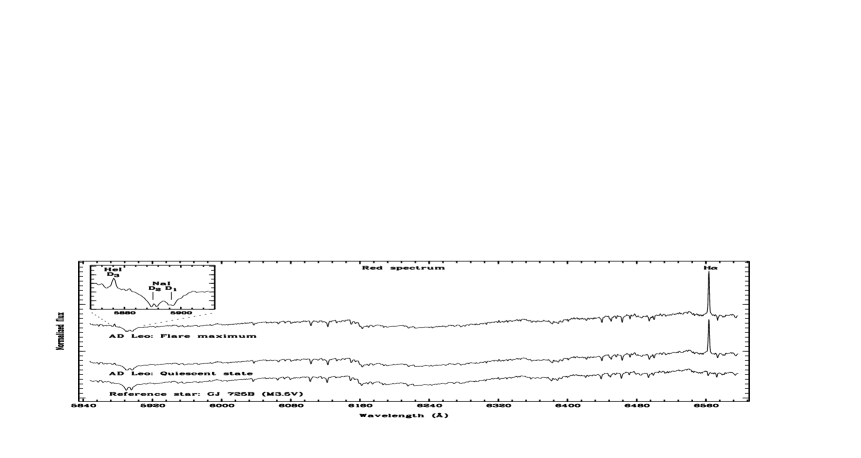
Figure 2: As Fig. 1 but for the spectra taken with the R1200Y grating, the strongest flare detected using this spectral configuration (flare 12, see $\S$ 3.1), and the reference star GJ 725B.

2 Observations and data reduction

The data were taken during the MUlti-SIte COntinuous Spectroscopy (MUSICOS) 2001 campaign. It involved observations at two sites: El Roque de los Muchachos Observatory from La Palma (Spain) and SAAO (South Africa). However, due to poor weather conditions, the only useful data were those taken at La Palma. This observing run was carried out with the 2.5 m Isaac Newton Telescope (INT) during 2 – 5 April 2001. The Intermediate Dispersion Spectrograph (IDS) was utilized together with the 2148x4200 EEV10a CCD detector. Two gratings were used: R1200B (every night) and R1200Y (second half of the last night). The wavelength covered by R1200B (blue spectrum) ranges from 3554 Å to 5176 Å (including the Balmer lines from H$\beta$ to H₁₁ as well as the Ca ii H & K and He i 4026 Å lines). The reciprocal dispersion of these spectra is 0.48 Å/pixel. The wavelength covered by R1200Y (red spectrum) ranges from 5527 Å to 7137 Å (including the H$\alpha$, Na i D₁ & D₂ and He i D₃ lines), being the reciprocal dispersion 0.47 Å/pixel. The spectral resolution, determined as the full width at half maximum (FWHM) of the arc comparison lines, is 1.22 Å for the blue region and 1.13 Å for the red one.

Figure 3: Temporal evolution of the $EW$ of the H$\beta$ line. The strongest observed flares are labeled.

Figure 4: As Fig. 3 but for the H$\alpha$ line. The observed flares have been numbered following the order in Fig. 3.

We took series of spectra with short exposure times: from 15 to 300 s for R1200B and from 5 to 120 s for R1200Y. The spectra in each series were separated only by the CCD readout time (less than 60 s) in order to obtain the highest temporal resolution as possible. During 4 nights, a total of 459 spectra of AD Leo were obtained with R1200B and 189 with R1200Y. The observing log (Table 1) lists: the number of spectra taken every night ($N$), the universal time (UT) at the beginning and end of the AD Leo observations, the minimum and maximum exposure time ($t_{\rm exp}$) of the spectra, and the signal-to-noise ratio ($SNR$) of the continuum near each line region. These quantities are given for both gratings (R1200B and R1200Y). Note that, despite the short exposure times, the $SNR$ is large enough to perform a reliable analysis.

The reduction has been done following the standard procedure: bias and dark subtraction, flat-field correction using exposures of a tungsten lamp, cosmic rays correction, and sky background subtraction from the region of the aperture chosen for doing an optimal extraction of each spectrum. The software packages of IRAF have been used. The wavelength calibration has been done by using spectra of Cu–Ar lamps. Finally, all the spectra have been normalized to their maximum flux value of the observed continuum.

3 Analysis of the observations

In Fig. 1 we have plotted the observed blue spectrum of AD Leo in its quiescent state (minimum observed emission level) and at the maximum of the strongest flare detected with the R1200B grating (flare 2, see $\S$ 3.1). Fig. 2 is similar to Fig. 1 but for the red spectra, taken with the R1200Y grating, and the strongest flare detected with this spectral configuration (flare 12, see $\S$ 3.1). In addition, the spectra of Gl 687B and GJ 725B have been plotted as examples of inactive stars with a spectral type and luminosity class (M3.5V) very similar to those of AD Leo (M3V). Note that the origin of the Y-axis is different for every spectrum in order to avoid the overlapping between them.

Table 2: Minimum and maximum relative error in the $EW$ of the different chromospheric lines.

Night	$\bigtriangleup EW_{\rm rel}$ (%)
	(min–max)
	H$\beta$	H$\gamma$	H$\delta$	He i $\lambda$4026Å	Ca ii K	Ca ii H+H$\epsilon$	H8	H9	H10	H11	H$\alpha$	Na i D1	Na i D2	He i D3
1	10–13	6–9	8–14	20–46	5–8	5–8	9–20	9–17	11–24	16–37	–	–	–	–
2	9–15	6–10	7–17	19–57	5–9	5–10	9–23	9–22	12–34	17–62	–	–	–	–
3	10–17	6–12	8–20	24–109	5–13	5–13	10–28	9–29	12–41	17–61	–	–	–	–
4	10–20	6–15	8–23	27–152	5–14	6–15	10–34	10–39	12–56	18–145	9–20	2–5	1–5	32–328

AD Leo shows a high level of chromospheric activity. A strong emission in the Balmer series and the Ca ii H & K lines is observed even in its quiescent state (see Fig. 1 and 2). The greatest emission in these lines is found at the maximum of the detected flares. The He i D₃ and He i 4026 Å lines also show emission above the continuum, which is more noticeable during the strongest flares. The Na i D₁ & D₂ absorption lines only present a slight filled-in profile in the quiescent state, though a low emission is observed in their core during flares. High resolution spectroscopic observations of the quiescent state of AD Leo confirm the presence of chromospheric emission lines that range from a weak emission in the center of the Ca ii IRT and the Na i D₁ & D₂ lines to a strong emission in the He i D₃, Mg ii h & k, Ca ii H & K and H i Balmer lines (Pettersen & Coleman 1981; Doyle 1987; Crespo-Chacón et al. 2006). In addition, Sundland et al. (1988) suggested that Balmer lines are the most important components to chromospheric radiation loss.

AD Leo is well-known for having strong flares (see, for example, Hawley & Pettersen 1991). However, after overlapping the normalized spectra and comparing the depth of the absorption lines and the shape of the continuum, we have not detected any noticeable continuum change (see also Fig. 1 and 2). Therefore the flares analyzed in this work are non white-light flares and, within the studied wavelength range, they only affect the emission in the chromospheric lines. Despite this kind of flares is the most typical in the Sun, in which no detectable signature in white-light is generally observed, very few such events had been previously detected on stars (see Butler et al. 1986; Houdebine 2003). Conversely to the Sun, stellar non white-light flares have been seldom observed because very little time has been dedicated to spectroscopy in comparison to photometry. However, Houdebine (1992) suggested that the low frequency observed for stellar non white-light flares could be due to a strong contrast effect. In other words, many flares have been detected as white-light flares on dMe stars because of the relative weakness of their photospheric background, but they would have been classified as non white-light flares on the Sun because of its much higher photospheric background.

3.1 Equivalent widths

The equivalent width ($EW$) of the observed chromospheric lines has been measured very carefully in order to detect possible weak flares in our observations. Two methods have been tried out. The first one consists of obtaining the $EW$ with the routine SPLOT included in IRAF, taking exactly the same wavelength limits for each line in all the spectra. The second method uses the routine SBANDS of IRAF, which generally introduces less noise in the $EW$ measurement because of taking into account a larger number of points to calculate the continuum value. For this reason, we only present the results obtained with SBANDS. Note that the line regions have been taken wide enough to include the enhancement of the line wings during flares.

SBANDS uses Eq. 1 to obtain the $EW$ of a line; where $W_{{\rm l}}$ is the width at the base of the line, $d$ is the reciprocal dispersion (pixel size in Å), ${F_{{\rm c},{\rm i}}}$ is the flux per pixel in the continuum under the line, ${F_{{\rm l},{\rm i}}}$ is the observed flux in the pixel i of the line, and $n$ is the number of pixels within the line region.

$$EW={W_{{\rm l}}-\frac{d}{F_{{\rm c},{\rm i}}}\ \displaystyle{\sum_{{\rm i}=1}^{{\rm i}=n}F_{{\rm l},{\rm i}}}}$$ (1)

The $EW$ uncertainty has been estimated using Eq. 2. We have considered $\bigtriangleup W_{{\rm l}}=0\leavevmode\nobreak\ {\rm\AA}$ and $\bigtriangleup d=0.01\leavevmode\nobreak\ {\rm\AA/pixel}$. Eq. 2 has been obtained by applying the standard quadratic error propagation theory to Eq. 1, taking into account that $n=W_{{\rm l}}/d$ and assuming $\bigtriangleup F_{{\rm l},{\rm i}}\approx\bigtriangleup F_{{\rm c},{\rm i}}=F_{{\rm c},{\rm i}}/{\rm SNR}$.

$$\bigtriangleup EW=\sqrt{\left(C_{1}\right)^{2}+\left(C_{2}\right)^{2}+\left(C_{3}\right)^{2}+\left(C_{4}\right)^{2}}$$ (2)

where

$$C_{1}=\frac{\partial EW}{\partial W_{{\rm l}}}\bigtriangleup W_{{\rm l}}=\bigtriangleup W_{{\rm l}}$$

$$C_{2}=\frac{\partial EW}{\partial d}\bigtriangleup d=\frac{EW-W_{{\rm l}}}{d}\bigtriangleup d$$

$$C_{3}=\frac{\partial EW}{\partial F_{{\rm c},{\rm i}}}\bigtriangleup F_{{\rm c},{\rm i}}=\frac{W_{{\rm l}}-EW}{{\rm SNR}}$$

$$C_{4}=\frac{\partial EW}{\partial F_{{\rm l},{\rm i}}}\bigtriangleup F_{{\rm l},{\rm i}}=\frac{\sqrt{W_{{\rm l}}\ d}}{{\rm SNR}}$$

Table 3: $JD$ of the flare onset ($JD_{\rm start}$), total duration of the detected flares and length of their phases (seen in the H$\beta$ line in the case of flares 1 to 11 and seen in the H$\alpha$ line in the case of flares 12 to 14). The time delay between the maximum of the chromospheric lines and the one of H$\beta$ or H$\alpha$, depending on the spectral configuration, is also shown. Blanks are given when the beginning, maximum and/or end of the flare was not observed in the line under consideration.

Flare	$JD_{\rm start}$ (days)	Duration (min)				Delay of the maximum (min)
	(2452000+)
		Total	Impulsive phase	Gradual decay		Ca ii K	He i 4026 Å
		(H$\beta$)	(H$\beta$)	(H$\beta$)
1	2.513$\pm$0.003	–	13$\pm$7	–		–	0$\pm$6
2	3.3903$\pm$0.0016	25$\pm$4	11$\pm$5	14$\pm$4		0$\pm$5	0$\pm$5
3	3.5321$\pm$0.0016	–	10$\pm$4	–		0$\pm$4	0$\pm$4
4	3.5608$\pm$0.0013	31$\pm$3	10$\pm$4	22$\pm$3		0$\pm$4	0$\pm$4
5	4.3781$\pm$0.0010	18$\pm$4	6$\pm$2	11$\pm$3		0$\pm$1	–
6	4.4193$\pm$0.0005	22$\pm$1	4$\pm$2	17$\pm$2		5$\pm$3	0$\pm$3
7	4.4804$\pm$0.0010	25$\pm$2	9$\pm$3	16$\pm$2		3$\pm$2	1$\pm$2
8	4.5479$\pm$0.0009	–	10$\pm$2	–		1$\pm$1	1$\pm$1
9	4.5978$\pm$0.0005	17$\pm$2	5$\pm$1	12$\pm$2		2$\pm$1	–
10	–	–	–	–		–	–
11	5.3968$\pm$0.0005	14$\pm$1	1$\pm$1	12$\pm$1		3$\pm$1	–

Flare	$JD_{\rm start}$ (days)	Duration (min)				Delay of the maximum (min)
	(2452000+)
		Total	Impulsive phase	Gradual decay		Na i D1, D2	He i D3
		(H$\alpha$)	(H$\alpha$)	(H$\alpha$)
12	5.5341$\pm$0.0003	31$\pm$2	5.9$\pm$0.9	25$\pm$2		0.9$\pm$0.9	–
13	5.5763$\pm$0.0005	14$\pm$1	2$\pm$1	12$\pm$1		1$\pm$1	1$\pm$1
14	–	–	–	–		–	–

Table 2 shows the minimum and maximum values of the relative error in $EW$ ($\bigtriangleup EW_{\rm rel}$) for each chromospheric line and every night. The $\bigtriangleup EW_{\rm rel}$ of the Ca ii H & K, Na i D₁ & D₂, H$\beta$, H$\gamma$ and H$\delta$ lines is between 1 % and 20 %. For H₈ and H₉ the $\bigtriangleup EW_{\rm rel}$ is less than 40 %, while for H₁₀ and H₁₁ is higher than the uncertainty estimated for the other Balmer lines (up to 50 % in the case of H₁₀ and even larger than 100 % in the case of H₁₁). In addition, the $\bigtriangleup EW_{\rm rel}$ of He i D₃ and He i 4026 Å is frequently greater than 100 %. For this reason, the results obtained for the He i lines are less reliable. Besides, because of the short exposure times and the relative faintness of AD Leo in the blue, the region blueward H₁₀ is usually too noisy for reliable measurements.

The observed flares have been detected using the H$\beta$ and H$\alpha$ lines (for the blue and red spectra, respectively). H$\beta$ and H$\alpha$ have been chosen because they suffer from large variations during flares and are the chromospheric lines with the best $SNR$ in each spectral configuration.

Fig. 3 shows the temporal evolution found for the $EW$ of the H$\beta$ line. The observed flares are marked with numbers. Other smaller changes can also be seen. The temporal evolution found for the $EW$ of the H$\alpha$ line is given in Fig. 4. No strong variations have been observed during our spectroscopic monitoring. However, 14 short and weak flares have been detected: 11 among the blue spectra and 3 among the red ones. The Julian Date ($JD$) at the beginning of each flare ($JD_{\rm start}$) is shown in Table 3. These flares have been also observed in the other chromospheric lines. Nevertheless, it is more difficult to distinguish between flares and noise for lower $SNR$ and/or weaker lines. In addition, a modulation with a period of $\sim$ 2 days is also observed in the quiescent emission of AD Leo, though the photometric period of this star was found to be 2.7 days (Spiesman & Hawley 1986).

Table 4: $EWRQ$ at flare maximum ($EWRQ_{\rm max}$) for the different chromospheric lines. Blanks are given when the flare maximum was not detected in the line under consideration. Flares with no maximum data in any line have been omitted.

Flare	$EWRQ_{\rm max}$
	H$\beta$	H$\gamma$	H$\delta$	H8	H9	H10	H11	Ca ii H + H$\epsilon$	Ca ii K	He i 4026 Å
1	1.26$\pm$0.18	1.28$\pm$0.11	1.47$\pm$0.17	1.53$\pm$0.22	1.52$\pm$0.20	1.7$\pm$0.3	1.6$\pm$0.4	1.16$\pm$0.09	–	1.5$\pm$0.5
2	1.65$\pm$0.25	1.52$\pm$0.14	2.0$\pm$0.3	2.0$\pm$0.3	1.8$\pm$0.3	1.5$\pm$0.3	2.0$\pm$0.7	1.30$\pm$0.11	1.14$\pm$0.09	1.7$\pm$0.6
3	1.09$\pm$0.19	1.06$\pm$0.10	1.10$\pm$0.17	1.11$\pm$0.21	1.13$\pm$0.22	0.99$\pm$0.23	1.0$\pm$0.4	1.1$\pm$0.1	1.01$\pm$0.09	1.3$\pm$0.5
4	1.23$\pm$0.20	1.25$\pm$0.12	1.44$\pm$0.21	1.5$\pm$0.3	1.5$\pm$0.3	1.6$\pm$0.3	1.6$\pm$0.6	1.13$\pm$0.10	1.06$\pm$0.09	1.2$\pm$0.5
5	1.08$\pm$0.20	1.08$\pm$0.13	1.14$\pm$0.21	1.1$\pm$0.3	1.1$\pm$0.3	1.0$\pm$0.3	1.5$\pm$0.6	1.06$\pm$ 0.13	1.01$\pm$0.12	–
6	1.4$\pm$0.3	1.34$\pm$0.17	1.6$\pm$0.3	1.8$\pm$0.5	1.4$\pm$0.4	1.5$\pm$0.5	1.3$\pm$0.5	1.23$\pm$0.16	1.14$\pm$0.13	1.6$\pm$0.9
7	1.32$\pm$0.24	1.32$\pm$0.17	1.5$\pm$0.3	1.4$\pm$0.4	1.7$\pm$0.4	1.5$\pm$0.5	1.9$\pm$0.8	1.15$\pm$0.15	1.09$\pm$0.14	1.9$\pm$1.1
8	1.27$\pm$0.23	1.25$\pm$0.14	1.49$\pm$0.25	1.5$\pm$0.3	1.5$\pm$0.3	1.4$\pm$0.4	1.5$\pm$0.6	1.16$\pm$0.13	1.06$\pm$0.11	1.6$\pm$0.8
9	1.16$\pm$0.21	1.07$\pm$0.13	1.18$\pm$0.21	1.2$\pm$0.3	1.3$\pm$0.3	1.1$\pm$0.3	1.0$\pm$0.4	1.13$\pm$0.14	1.06$\pm$0.14	–
11	1.12$\pm$0.22	1.10$\pm$0.15	1.19$\pm$0.24	1.3$\pm$0.3	1.1$\pm$0.3	1.2$\pm$0.4	1.0$\pm$0.5	1.05$\pm$0.13	1.07$\pm$0.13	–

Flare	$EWRQ_{\rm max}$
	H$\alpha$	Na i D1	Na i D2	He i D3
12	1.09$\pm$0.15	0.95$\pm$0.04	0.95$\pm$0.03	–
13	1.13$\pm$0.18	0.98$\pm$0.04	0.98$\pm$0.04	1.5$\pm$1.1

We want to emphasize that the flare frequency is very high, and sometimes new flares take place when others are still active (see, for example, flares 8 and 11 and the points before flares 2 and 7 in Fig. 3). It is also remarkable that the flares in night 4 seem to erupt over the gradual decay phase of other stronger flare (Fig. 4). For calculating the flare frequency we have taken the total observed time as the sum of UT_end – UT_start for all the nights (see Table 1). Note that, within a night, the series of observations are not continuous in time. Therefore the flare frequency should be greater than the obtained one. This implies that the flare activity of AD Leo, found from the variations of the chromospheric emission lines, is $>$ 0.71 flares/hour. This value is slightly higher than those that other authors measured by using photometry: Moffett (1974) observed 0.42 flares/hour, Pettersen et al. (1984) detected 0.57 flares/hour, and Konstantinova-Antova & Antov (1995) found 0.33 - 0.70 flares/hour. Given that the detected flares are non white-light flares, we conclude that non white-light flares may be more frequent on stars than white-light flares, as observed in the Sun. In fact, as the total time of the gaps between the series of observations is similar to the total real observed time, the flare activity of AD Leo could even be the double of that obtained. As far as we know, this is the first time that such a high flare frequency is inferred from the variation of the chromospheric emission lines.

3.2 Equivalent widths relative to the quiescent state

In order to compare the behaviour of the different chromospheric lines, we have used the equivalent width relative to the quiescent state ($EWRQ$), defined as the ratio of the $EW$ to the $EW$ in the quiescent state. Fig. 5 and 6 show the $EWRQ$ of several lines for a representative sample of the detected flares (those in which all the phases have been observed). The chromospheric lines plotted in these two figures are those with less uncertainty in the $EW$ measurement. We can observe two different kinds of flares: for some of them (see flares 6, 9, 11, 12 and 13) the gradual decay phase of the Balmer lines is much longer than the impulsive phase; in contrast, other flares (2, 4, 5 and 7) are less impulsive. This resembles the classification of solar flares made by Pallavicini et al. (1977): eruptive flares or long-decay events and confined or compact flares. However, all these flares always show the same behaviour in the Ca ii H & K lines, that is a slow evolution throughout all the event. The evolution of the Na i D₁ & D₂, He i D₃ and He i 4026 Å lines is quite similar to that of the Balmer series. However, it is less clear for the He i lines because of having a very high error sometimes.

Figure 5: $EWRQ$ of the flares (detected using the R1200B grating) in which all the phases have been observed (lines: H$\beta$, H$\gamma$, H$\delta$, H₈, Ca ii H + H$\epsilon$, Ca ii K, He i 4026 Å).

Figure 6: As Fig. 5 but for the flares detected using the R1200Y grating (lines: H$\alpha$, Na i D₁, Na i D₂, He i D₃).

In some flares (5, 6, 11, 12 and 13) we can see two maxima in the Na i and Balmer lines, but it is not so evident for the He i and Ca ii lines. Sometimes variations at shorter time scales are also detected during the gradual decay phase, in which different peaks, decreasing in intensity, are observed in the $EWRQ$ (see, for instance, flare 12). This could be interpreted as the succession of different reconnection processes, decreasing in efficiency, within the same flare – following the original suggestion of Kopp & Pneuman (1976) – or as a series of flares originated as a result of wave disturbances coming along the stellar surface from the first flare region.

Table 3 contains: the total duration of the detected flares, the length of their impulsive and gradual decay phases, and the time delay between the maximum of each chromospheric line and that of H$\beta$ or H$\alpha$ (depending on the spectral configuration). The detected flares last from 14 $\pm$ 1 up to 31 $\pm$ 3 min. Regarding the first maximum of emission, we have found that the Balmer series reach it simultaneously while the rest of the lines are delayed. The delay is negligible for the He i and Na i lines ($\sim$ 1 min) but it is very evident for Ca ii H & K (up to 5 $\pm$ 3 min). It seems that this delay is greater for the flares with a shorter impulsive phase of the Balmer lines. However, the total duration of the flare does not seem to be related. For the first five flares, we cannot assume that the delay of the maximum is completely zero because their uncertainties, particularly those of He i 4026 Å, are even greater than the delay found in the other cases. The moment in which a line reaches its maximum is related to the height where the line is formed above the stellar surface. This is also related to the temperature that characterizes the formation of the line. According to the line formation models in stellar atmospheres, the Ca ii H & K lines are formed at deeper and cooler layers than the Balmer series. Therefore, the gas that is heated and evaporated into the newly formed loop after magnetic reconnection (Cargill & Priest 1983; Forbes & Malherbe 1986) cools and reaches the formation temperature of the Balmer series before the one of the Ca ii H & K lines. Houdebine (2003) found that the rise and decay times in the Ca ii K and H$\gamma$ lines obey good relationships, which implies that there is a well-defined underlying mechanism responsible for the flux time profiles in these lines.

Table 4 lists the $EWRQ$ of the chromospheric lines at their maximum in each flare ($EWRQ_{\rm max}$). The lower the wavelength, the greater $EWRQ_{\rm max}$ is found for the Balmer lines. However, H$\beta$ and H$\gamma$ have a very similar variation. For He i 4026 Å and He i D₃ the $EWRQ_{\rm max}$ is analogous to that of the Balmer series, whereas for the Ca ii H & K and Na i D₁ & D₂ lines is smaller. Our results show that the duration of flares tends to be larger when the $EWRQ_{\rm max}$ of the Balmer lines is greater. This effect is more noticeable for the less impulsive flares. Nevertheless, there are no clear relationships between the $EWRQ_{\rm max}$ of the other lines and the duration of the flare.

3.3 Line fluxes and released energy

In order to estimate the flare energy released in the observed chromospheric lines, we have converted the $EW$ into absolute surface fluxes and luminosities.

The absolute line fluxes ($F$) have been computed from the $EW$ measured for each line and its local continuum. The absolute flux of the continuum near each line has been determined making use of the method given by Pettersen & Hawley (1989). For AD Leo, they interpolate between the R and I filter photometric fluxes to estimate the observed flux in the continuum near 8850 Å. This value is then transformed into a continuum surface flux of $F$(8850 Å) = 6.5 $\times$ 10⁵ erg s^-1cm^-2Å^-1, using 0.44 $R_{\odot}$ for the radius and 0.203 arcsec for the parallax. Direct scaling from the flux-calibrated spectrum of AD Leo, showed by Pettersen & Hawley (1989), has allowed us to estimate the continuum surface fluxes near the emission lines of interest. We multiply this continuum value by the measured $EW$ to determine the line surface flux. The absolute fluxes of the Balmer lines at the different flare maxima ($F_{\rm max}$) are listed in Table 5. These values will be used in $\S$ 4 to calculate the Balmer decrements. Note that each $F_{\rm max}$ only shows the contribution of the flare to the surface flux (the contribution of the quiescent state has been subtracted). Since our aim is to isolate the contribution of the flares from the total emission, we have chosen the quiescent state for each of them as a pseudo-quiescent, that is the minimum emission level just before or after the flare. In this way, variations originated by other processes, which can contribute to the observed emission, are not taken into account. Even if these processes were magnetic reconnections within the same active region, assuming that the solar flare model is also applicable to the stellar case, the new emitting plasma would be placed in a different post-flare loop (Cargill & Priest 1983; Forbes & Malherbe 1986). Therefore, in first approximation, its physical properties (see $\S$ 4) could be separately studied.

We have also converted the absolute fluxes into luminosities ($L$). Table 6 lists the contribution of every flare to the energy released in the Balmer lines. The released energy has been calculated by numerically integrating the luminosity from the beginning to the end of the flare and subtracting the contribution of its corresponding pseudo-quiescent state. The energy released during the impulsive and gradual decay phases, which has been calculated in the same way, is given as well.

Table 5: Surface fluxes of the Balmer lines at flare maximum ($F_{\rm max}$). The contribution of the quiescent state has been subtracted. Flares with no maximum data in any line have been omitted.

Flare	$F_{\rm max}$ (105 erg s-1cm-2)
	H$\alpha$	H$\beta$	H$\gamma$	H$\delta$	H8	H9	H10	H11
1	–	0.90	0.64	0.56	0.29	0.23	0.109	0.070
2	–	1.82	1.10	0.90	0.47	0.33	0.108	0.105
3	–	0.34	0.19	0.15	0.08	0.053	0.011	0.013
4	–	0.70	0.52	0.41	0.22	0.17	0.120	0.079
5	–	0.34	0.23	0.19	0.10	0.04	0.079	0.061
6	–	1.19	0.70	0.62	0.32	0.16	0.084	0.040
7	–	0.94	0.62	0.43	0.19	0.25	0.076	0.090
8	–	0.74	0.48	0.42	0.16	0.14	0.072	0.053
9	–	0.57	0.27	0.30	0.11	0.11	0.070	0.036
11	–	0.35	0.07	0.18	0.08	0.03	0.050	0.010
12	1.10	–	–	–	–	–	–	–
13	1.40	–	–	–	–	–	–	–

Table 6: Energy released in the Balmer lines during every flare phase. The total released energy is also shown. The contribution of the quiescent state has been subtracted. We have omitted the flares with no data about their beginning, maximum and end.

Flare	Phase	Released energy (1029 erg)
		H$\alpha$	H$\beta$	H$\gamma$	H$\delta$	H8	H9	H10	H11
1	Impulsive	–	2.5	1.2	1.6	0.8	0.7	0.3	0.2
	Gradual	–	–	–	–	–	–	–	–
	Total	–	–	–	–	–	–	–	–
2	Impulsive	–	3.3	2.3	1.4	0.9	0.9	0.2	0.3
	Gradual	–	4.9	3.1	2.0	1.2	1.2	0.4	0.5
	Total	–	8.2	5.4	3.4	2.2	2.1	0.6	0.7
3	Impulsive	–	1.2	0.7	0.7	0.3	0.2	0.1	0.0
	Gradual	–	–	–	–	–	–	–	–
	Total	–	–	–	–	–	–	–	–
4	Impulsive	–	1.9	1.3	0.9	0.6	0.5	0.4	0.3
	Gradual	–	2.2	1.6	0.6	0.9	0.5	0.5	0.5
	Total	–	4.1	3.0	1.5	1.5	1.1	0.9	0.8
5	Impulsive	–	0.6	0.2	0.3	0.2	0.1	0.3	0.2
	Gradual	–	1.0	0.6	0.4	0.2	0.1	0.4	0.2
	Total	–	1.5	0.8	0.7	0.4	0.2	0.7	0.4
6	Impulsive	–	1.5	0.7	0.9	0.5	0.2	0.1	0.0
	Gradual	–	6.2	3.3	3.1	1.8	1.0	0.3	0.1
	Total	–	7.7	3.9	4.0	2.3	1.2	0.4	0.1
7	Impulsive	–	1.8	1.2	1.1	0.4	0.5	0.2	0.2
	Gradual	–	5.4	3.4	3.2	1.3	0.8	0.6	0.6
	Total	–	7.2	4.6	4.4	1.7	1.2	0.8	0.9
8	Impulsive	–	2.0	1.3	1.0	0.4	0.4	0.2	0.1
	Gradual	–	–	–	–	–	–	–	–
	Total	–	–	–	–	–	–	–	–
9	Impulsive	–	0.6	0.4	0.3	0.0	0.0	0.1	0.0
	Gradual	–	1.5	0.9	0.7	0.1	0.1	0.3	0.2
	Total	–	2.1	1.3	1.0	0.1	0.1	0.5	0.2
11	Impulsive	–	0.2	0.1	0.1	0.0	0.0	0.0	0.0
	Gradual	–	1.8	0.6	1.2	0.2	0.2	0.4	0.1
	Total	–	2.0	0.7	1.3	0.2	0.2	0.5	0.1
12	Impulsive	3.1	–	–	–	–	–	–	–
	Gradual	10.3	–	–	–	–	–	–	–
	Total	13.4	–	–	–	–	–	–	–
13	Impulsive	1.0	–	–	–	–	–	–	–
	Gradual	6.5	–	–	–	–	–	–	–
	Total	7.5	–	–	–	–	–	–	–

3.4 Line profiles and asymmetries

We focus this section on the Balmer series and Ca ii H & K lines. The intermediate spectral resolution of the observations has not allowed us to study the profile of the He i and Na i lines because of their low intensity.

We have plotted the temporal evolution of the observed line profiles during the detected flares (see the examples given in Fig. 7). No evidence for line-shifts has been found. However, the reported flares may be too weak for measuring line-shifts using the available spectral resolution (see $\S$ 2). It seems that flares affect the core of the lines before the wings. The emission in both of them (core and wings) increases during the impulsive phase, shows the largest value when the $EWRQ$ of the line reaches the maximum, and decreases during the gradual decay. The emission in the wings of the Ca ii H & K lines hardly rises during the observed flares, being only noticeable during the strongest ones (see Fig. 7). In fact, their broadening is negligible even at flare maximum. If the flare is too weak, as the flare 5, the profile of the Balmer lines shows the same behaviour as that found for the Ca ii H & K lines. In contrast, when the released energy is high enough to produce changes in the wings of the Balmer series (flares 2, 6 and 7), the core of these lines seems to rise up to a constant value (which is independent of the $EWRQ_{\rm max}$) whereas the emission in the wings depends on the flare energy. Table 7 lists the width at the base of the lines of interest during the quiescent state and the maximum of the strongest observed flare (flare 2). The fact that the width of the Ca ii lines is much less sensitive to flares than that of the Balmer lines suggests that the broadening may be due to the Stark effect (Byrne 1989; Robinson 1989). Nevertheless, mass motions can also be present (see below).

Figure 7: Evolution of the H_β (left) and Ca ii K (right) line profiles (solid line) during the strongest observed flare (flare 2), compared with the quiescent state (dotted line).

Fig. 8 shows, as an example, the bisector of the H$\beta$ and Ca ii K lines during the flare 2. The bisector of a line is defined as the middle points of the line profile taking points of equal intensity at both sides of the line (Toner & Gray 1988; López-Santiago et al. 2003).

The Balmer lines are broadened during the early-flare phases and the broadening decreases along the flare evolution (see Fig. 7). Although the emission rises in both wings of the Balmer lines, the observed enhancement and broadening are bigger in the red wing. Therefore the Balmer lines show a red asymmetry during the detected flares, and the largest asymmetry is observed at flare maximum (see also the behaviour of the bisectors given in Fig. 8). Besides, the stronger the flare (flares 2 and 6) the greater this asymmetry is. The red asymmetry is also stronger in higher members of the Balmer series. We have used a two-Gaussian (narrow=N and broad=B) fit to model the Balmer lines at flare maxima. The B component appears red-shifted with respect to N. For example, at the maximum of flare 2 the distance between both components increases from 0.4 Å in the case of H$\beta$ up to 1.5 Å in H₈. Doyle et al. (1988) observed a similar effect during a flare on YZ CMi, finding that H$\gamma$ and H$\delta$ showed symmetrically broadened profiles while H₈ and H₉ showed predominantly red-shifted material. They suggested that within an exposure time as those used in this work (see Table 1) several downflows, corresponding to different flare kernels which brighten successively one after another, may be present in the stellar atmosphere. Every downflow would produce a red-shifted contribution to the Balmer lines, which would be larger for higher members of the Balmer series (see $\S$ 3.2). In addition, a smaller red asymmetry in the Balmer lines is also observed during the quiescent state of AD Leo.

Table 7: Width at the base of the chromospheric lines in the quiescent state and at the maximum of flare 2.

Line	Width at the base of the line
	Quiescent state	Maximum of flare 2
H$\beta$	5$\pm$1	13$\pm$1
H$\gamma$	4$\pm$1	6$\pm$1
H$\delta$	4$\pm$1	9$\pm$1
He i 4026 Å	1$\pm$1	1$\pm$1
Ca ii H + H$\epsilon$	4$\pm$1	6$\pm$1
Ca ii K	3$\pm$1	5$\pm$1
H8	3$\pm$1	6$\pm$1
H9	3$\pm$1	5$\pm$1
H10	3$\pm$1	3$\pm$1
H11	3$\pm$1	5$\pm$1

Figure 8: Evolution of the bisector of the H_β (left) and Ca ii K (right) lines during the strongest flare (flare 2). Note that only the minimum value of each bisector is placed on the $JD$ in which its respective spectrum was taken.

The Ca ii H & K lines are not usually broadened and do not show any asymmetry, excepting the case of the strongest flare, where little variations are observed (see Fig. 7 and 8).

There are several interpretations for the asymmetries. Broad Balmer emission wings have been observed during flares produced by very different kinds of stars, showing blue or red asymmetries (Doyle et al. 1988; Phillips et al. 1988; Eason et al. 1992; Houdebine et al. 1993; Gunn et al. 1994a; Abdul-Aziz et al. 1995; Abranin et al. 1998; Berdyugina et al. 1998; Montes et al. 1999; Montes & Ramsey 1999; López-Santiago et al. 2003) or no obvious line asymmetries (Hawley & Pettersen 1991). Broadened profiles and red asymmetries are important constraints on flare models (Pallavicini 1990). They can be attributed to plasma turbulence or mass motions in the flare region (see Montes et al. 1999; Fuhrmeister et al. 2005, and references therein). In solar flares, most frequently, a red asymmetry is observed in chromospheric lines. Taking into account that the flares reported in this work are like the most typical solar flares – non white-light flares – it was expected to find red asymmetries like those observed. However, evidences of blue asymmetries have been also reported during solar flares (Heinzel et al. 1994). Red asymmetries have been often interpreted as the result of chromospheric downward condensations (CDC) (see Canfield et al. 1990, and references therein). In fact, recent line profile calculations (Gan et al. 1993; Heinzel et al. 1994; Ding & Fang 1997) show that a CDC can explain both blue and red asymmetries. On the other hand, evidences of mass motions have been also reported during stellar flares. In particular, a large enhancement in the far blue wings of Balmer lines during the impulsive phase of a stellar flare was interpreted as high velocity mass ejection (Houdebine et al. 1990) or high velocity chromospheric evaporation (Gunn et al. 1994b), whereas red asymmetries in Balmer lines were reported by Houdebine et al. (1993) as evidence of CDC.

Finally, the small red asymmetry observed in the Balmer series during the quiescent state can be therefore interpreted as multiple CDC happening in the stellar atmosphere. These CDC may be produced by unresolved continuous low energy flaring.

4 Balmer decrement line modeling

Balmer decrements (flux ratio of higher members to H$\gamma$) have been frequently used to derive plasma densities and temperatures in the chromosphere of flare stars (Kunkel 1970; Gershberg 1974; Katsova 1990). Jevremović et al. (1998) developed a procedure (BDFP hereafter) to fit the Balmer decrements in order to determine some physical parameters in the flaring plasma. García-Alvarez et al. (2002); García-Alvarez et al. (2006) used the BDFP to obtain a detailed trace of physical parameters during several flares.

Table 8: Physical parameters obtained for the observed flares. The area and stellar surface percentage covered by these flares are also shown.

Flare	Date	UT	log $\tau_{Ly\alpha}$	log $n_{\rm e}$	log $T_{\rm e}$	log $T_{\rm us}$	Area	Surface
							($\times$ 1019 cm2)	(%)
1	03/04/01	00:30	3.71	13.75	4.31	4.13	1.17	0.40
2	03/04/01	21:32	4.62	13.79	4.07	3.99	6.79	2.30
3	04/04/01	00:55	4.18	14.22	4.09	3.90	1.45	0.49
4	04/04/01	01:36	3.78	13.95	4.30	3.98	0.89	0.30
5	04/04/01	21:11	4.54	13.79	4.12	4.02	0.76	0.26
6	04/04/01	22:08	4.43	14.12	4.07	4.04	3.14	1.07
7	04/04/01	23:41	4.41	14.39	4.09	4.02	2.13	0.72
8	05/04/01	01:18	4.15	13.78	4.17	3.98	2.12	0.72
9	05/04/01	02:25	3.60	13.88	4.38	4.09	0.36	0.12

The BDFP is based on the solution of the radiative transfer equation. It uses the escape probability technique (Drake 1980; Drake & Ulrich 1980) and a simplified picture of the flaring plasma as a slab of hydrogen with an underlying thermal source of radiation which causes photoionization. This source represents a deeper layer in the stellar atmosphere, which is exposed to additional heating during flares. For a detailed description of the physical assumptions made by the BDFP, see $\S$ 4.1 of García-Alvarez et al. (2002). The BDFP minimizes the difference between the observed and calculated Balmer decrements using a multi-directional search algorithm (Torczon 1991, 1992). This allows us to find the best possible solution for the Balmer decrements in a four dimensional parameter space, where the parameters are: electron temperature ($T_{\rm e}$), electron density ($n_{\rm e}$), optical depth in the Ly$\alpha$ line ($\tau_{Ly\alpha}$), and temperature of the underlying source or background temperature ($T_{\rm us}$). Although the temperature of the underlying source could be a free parameter in our code, we have fixed a lower limit at 2500 K for numerical stability reasons. The best solution for the Balmer decrements allows us to calculate the effective thickness of the slab of hydrogen plasma and the total emission measure per unit volume (see expressions given by Drake & Ulrich 1980). With these quantities we are also able to determine the surface area of the emitting plasma – volume/thickness – taking into account that the volume is the ratio of the observed flux in the H$\beta$ line to the total emission measure (also in this line) per unit volume.

4.1 Physical parameters of the observed flares

We apply the BDFP to the flares observed on AD Leo. The Balmer decrements for H$\gamma$, H$\delta$, H₈, H₉ and H₁₀ have been calculated at each flare maximum using the flare-only fluxes given in Table 5. We do not include higher Balmer lines due to both the difficulty in assigning their local continuum level and the very low $SNR$ in their spectral region.

Fig. 9 shows the observed and fitted Balmer decrements at the maximum of the detected flares. The strength of an optical flare is related to the slope of the fit solution for the Balmer decrements (García-Alvarez 2003): shallower slopes means stronger flares. The results after applying the BDFP are listed in Table 8. The flares 3, 6 and 7 have a relatively high electron density ($n_{\rm e}>$ 1 $\times$ 10¹⁴ cm^-3) compared with that found for the other flares (6 $\times$ 10¹³ cm^-3 $<$ $n_{\rm e}<$ 9 $\times$ 10¹³ cm^-3). The flare 3 also has the lowest background temperature ($T_{\rm us}$ $\sim$ 8000 K) which means that the ionization balance in this flare is even less radiatively dominated than in the other ones (9500 K $<T_{\rm us}$ $<$ 13500 K). The electron temperature of the observed flares ranges from 12000 K to 24000 K. Taking into account that H₁₀ seems to be out of the trend followed by the other Balmer decrements on flares 2 and 3 (see Fig. 9) we have also run the BDFP rejecting this point, obtaining no significant variations on the results (the logarithmic values of the physical parameters given in Table 8 change a mean of 5 %).

Figure 9: Observed Balmer decrements (squares) and optimum computed fits (solid line) at the maximum of the observed flares. The pseudo-quiescent state for each flare, as defined in $\S$ 3.3, is plotted as reference (dotted line). Note that the Balmer decrement for H₁₀ is out of the plotted region in flare 3, but it has been taken into account for doing the fit.

In addition, we have used the fit solutions for calculating the surface area covered by the flaring plasma. The values, which are between 3.6 $\times$ $10^{18}$ cm² and 6.8 $\times$ 10¹⁹ cm², are shown in Table 8. We find that all the observed flares cover less than 2.3 % of the projected stellar surface ($\pi R^{2}$).

All the obtained physical parameters are consistent with previously derived values for stellar flares. These flares are also similar in size and strength to those analyzed in previous works based on the same code (García-Alvarez 2003; García-Alvarez et al. 2002; García-Alvarez et al. 2006).

5 Discussion and conclusions

The star AD Leo has been monitored using high temporal resolution during 4 nights (2 – 5 April 2001). More than 600 intermediate resolution spectra have been analyzed in the optical wavelength range. Although large variations have not been observed, we have found frequent short (duration between 14 $\pm$ 1 and 31 $\pm$ 3 min) and weak (released energy in H$\beta$ between 1.5 $\times$ 10²⁹ and 8.2 $\times$ 10²⁹ erg) flares. Most of these flares are even weaker than those observed on AD Leo by Hawley et al. (2003). All the detected flares have been inferred from the variation in the $EW$ of different chromospheric lines, which has been measured using a very accurate method. Given that the continuum does not change during these events, they can be classified as non white-light flares, which so far represent the kind of flares least known on stars.

The observed flare activity is $>$ 0.71 flares/hour, which is slightly larger than the values that other authors obtained for this star by using photometry. As far as we know, it is the first time that such a high flare frequency is inferred from the variation of the chromospheric lines. In fact, AD Leo seems to be continuously flaring since we have detected 14 moderate flares and a great number of smaller events that appear superimposed on them. Given that the energy distribution of flares was found to be a power law (Datlowe et al. 1974; Lin et al. 1984) of the form ${dN}/{dE}=kE^{-\alpha}$ – where $dN$ is the number of flares (per unit time) with a total energy (thermal or radiated) in the interval [$E$, $E+dE$], and $\alpha$ is greater than 0 – we can expect very weak flares occurring even more frequently than the observed ones. Therefore our results can be interpreted as an additional evidence of the important role that flares can play as heating agents of the outer atmospheric stellar layers (Güdel 1997; Audard et al. 2000; Kashyap et al. 2002; Güdel et al. 2003; Arzner & Güdel 2004).

A total of 14 flares have been studied in detail. The Balmer lines allow to distinguish two different morphologies: some flares show a gradual decay much longer than the impulsive phase while another ones are less impulsive. This resembles the two main types of solar flares (eruptive and confined) described by Pallavicini et al. (1977). However, the Ca ii H & K lines always show the same behaviour and their evolution is less impulsive than that found for the Balmer lines. The two maxima and/or weak peaks, observed sometimes during the detected flares, can be interpreted as the succession of different magnetic reconnection processes, which would be originated as consequence of the disturbance produced by the original flare, as Kopp & Pneuman (1976) suggested for the Sun. The Ca ii H & K lines reach the flare maximum after the Balmer series. It seems that the time delay is higher when the impulsive phase of the Balmer lines is shorter. The moment in which a line reaches its maximum is related to the temperature that characterizes the formation of the line and, therefore, is also related to the height where the line is formed. During the detected flares, the relative increase observed in the emission of the Balmer lines is greater for lower wavelengths. We have also found that, not only the detected flares are like the most typical solar flares (non white-light flares), the asymmetries observed in chromospheric lines (red asymmetries) are also like the most frequent asymmetries observed in the Sun during flares. The detected broad Balmer emission wings and red asymmetries can be attributed to plasma turbulence, mass motions or CDC. The Ca ii H & K lines seem to be less affected by flare events and their broadening is negligible. A small red asymmetry in the Balmer series is also observed during the quiescent state, which could be interpreted as multiple CDC probably due to continuous flaring of very low energy.

Figure 10: Flare duration, stellar surface and temperature of the underlying source at flare maximum vs. energy released in H$\beta$ during the detected flares.

Figure 11: As Fig. 10 but vs. the flux emitted in H$\beta$ at flare maximum. The top panel has been added to show the relation between this flux and the energy released in H$\beta$.

In addition, we have used the Balmer decrements as a tracer of physical parameters during flares by using the model developed by Jevremović et al. (1998). The physical parameters of the flaring plasma (electron density, electron temperature, optical thickness and temperature of the underlying source), as well as the covered stellar surface, have been obtained. The electron densities found for the analyzed flares (6 $\times$ 10¹³ cm^-3 – 2 $\times$ 10¹⁴ cm^-3) are in general agreement with those that other authors find by using semi-empirical chromospheric modeling (Hawley & Fisher 1992a, b; Mauas & Falchi 1996). The electron temperatures are between 12000 K and 24000 K. The temperature of the background source ranges from 8000 K to 13500 K. All the obtained physical parameters are consistent with previously derived values for stellar flares. The areas – no larger than 2.3 % of the projected stellar surface – are comparable with the size of other solar and stellar flares (Tandberg-Hanssen & Emslie 1988; García-Alvarez 2003; García-Alvarez et al. 2002; García-Alvarez et al. 2006).

We have also analyzed the relationships between the flare parameters. The released energy is correlated with the flare duration and the area covered by the flaring plasma, but not with the temperature of the underlying source (see Fig. 10). These results are in general agreement with those found by Hawley et al. (2003) using only 4 flares and a different method for obtaining the physical parameters. We have found a clear relation between the released energy and the flux at flare maximum (see Fig. 11). Besides, the higher the flux, the longer the flare. This flux is also correlated with the area covered by the emitting plasma at flare maximum, but not with the temperature of the underlying source (Fig. 11). No correlations between the area, temperature and duration have been found: i.e. these parameters seem to be independent. The magnetic geometry seems to be a very important factor in flares: firstly, the flare duration can be related to the loop length, as in X-rays (see review by Reale 2002), in the sense that a fast decay implies a short loop and a slow decay a large loop; and secondly, the flare area can be related to the loop width, because the surface covered by the Balmer emitting plasma would be the projected area of the flaring loops. On the other hand, the temperature of the underlying source could be related to the depth of the layer reached by the flare accelerated particles, which is also related to the energy released through magnetic reconnection. For explaining the fact that the temperature of the underlying source seems to be well-defined and independent of the flare energy (see Fig. 10 and 11), we suggest that larger energies may imply more energetic particles and therefore larger depths, but not necessarily higher temperatures.

This work has extended the current number of stellar flares analyzed using high temporal resolution and good quality spectroscopic observations. However, there is still need for new data of this type to trace the behaviour of the physical parameters throughout these events. This will help us to understand the nature of flares on dMe stars. Finally, higher spectral resolution would be also desirable in order to study the changes that take place in stellar atmospheres during flares.