Dissipative or conservative cosmology with dark energy?

Abstract

All evolutional paths for all admissible initial conditions of FRW cosmological models with dissipative dust fluid (described by dark matter, baryonic matter and dark energy) are analyzed using dynamical system approach. With that approach, one is able to see how generic the class of solutions leading to the desired property – acceleration – is. The theory of dynamical systems also offers a possibility of investigating all possible solutions and their stability with tools of Newtonian mechanics of a particle moving in a 1-dimensional potential which is parameterized by the cosmological scale factor. We demonstrate that flat cosmology with bulk viscosity can be treated as a conservative system with a potential function of the Chaplygin gas type. We characterize the class of dark energy models that admit late time de Sitter attractor solution in terms of the potential function of corresponding conservative system. We argue that inclusion of dissipation effects makes the model more realistic because of its structural stability. We also confront viscous models with SNIa observations. The best fitted models are obtained by minimizing the $\chi^{2}$ function which is illustrated by residuals and $\chi^{2}$ levels in the space of model independent parameters. The general conclusion is that SNIa data supports the viscous model without the cosmological constant. The obtained values of $\chi^{2}$ statistic are comparable for both the viscous model and $\Lambda$CDM model. The Bayesian information criteria are used to compare the models with different power law parameterization of viscous effects. Our result of this analysis shows that SNIa data supports viscous cosmology more than the $\Lambda$CDM model if the coefficient in viscosity parameterization is fixed. The Bayes factor is also used to obtain the posterior probability of the model.

I Introduction

Several astronomical observations, since observations of distant supernova type Ia Riess et al. (1998); Perlmutter et al. (1999) and cosmic microwave background anisotropy measurements Spergel et al. (2003); Tegmark et al. (2004), have indicated that our Universe is currently undergoing an accelerating phase of expansion. If we assume that the Friedmann equation with perfect fluid source is valid then our Universe is in acceleration phase due to the presence of matter with negative pressure violating the strong energy condition (dark energy). While there are several candidates for description of dark energy like an evolving scalar field (referred to as quintessence) Ratra and Peebles (1988), generalized Chaplygin gas Gorini et al. (2003); Biesiada et al. (2005) or phantom dark energy Caldwell (2002); Da̧browski et al. (2003) the most obvious candidate for such a component of the dark energy seems to be the cosmological constant Weinberg (1989). Hence we obtain the most simple explanation of current universe which require two dark components, namely non-relativistic dust (dark and baryonic matter) contributing about 30% of the total energy density (which is clustering gravitationally at small scales) and second component (dark energy) which dominate at large scales and is smoothly distributed with constant density. Unfortunately it is only some kind of effective theory which offers description of present observations rater then its understanding. For example it remains to understand why the value of cosmological constant obtained from observations of SNIa is so small in comparison with the vacuum energy (Planck mass scale). It is the main reason for looking for alternative explanation of observational data of distant supernovae. There have appeared many models that make use of new physics which may arise as a consequence of embedding of our universe in a more dimensional universe which accelerates due to some additional term in the Friedmann equation rather than dark energy contribution Deffayet et al. (2002).

In this work we discuss the possibility of the dark energy being represented by viscous fluid which is characterized by the presence of bulk viscosity coefficient $\xi=-(1/3)\partial p_{\text{eff}}/\partial H$ in the effective equation of state. Because we assume homogeneity and isotropy, only bulk viscosity effects may be important under such symmetry condition. FRW models filled with a non-ideal (dissipative) fluid were investigated in several papers in which bulk viscosity was parameterized by an additional term in pressure $p\to p_{\text{eff}}=p-3\xi H$, where $\xi$ is the bulk viscosity coefficient, usually parameterized, following Belinskii, as power law $\xi(\rho)=\bar{\alpha}\rho^{m}$, where $\rho$ is the energy density and $\bar{\alpha}$ and $m$ are constants Belinskii and Khalatnikov (1975); Belinskii et al. (1979); Chimento and Jakubi (1993); van Elst and Tavakol (1994). While we know since the classical papers of Murphy Murphy (1973) and Heller Heller et al. (1973) that bulk viscosity effects can generate an accelerating phase of expansion the idea that the present acceleration epoch is driven by some kind viscous fluid is being explored recently Fabris et al. (2006). Wilson et al. Wilson et al. (2007) discussed a cosmology in this cold dark matter particle decay into relativistic particles and argued such a decay could lead naturally to bulk viscosity modelled by effective negative pressure.

The main aim of the paper is to investigate the possibility of explaining the present accelerating expansion of the Universe in terms of bulk viscosity with the background of models with Robertson-Walker symmetry, basing on analogy with the cosmology with the Chaplygin gas and dynamical system methods. We show that the non-flat FRW dissipative models can treated as a perturbed dynamical systems of the Newtonian type.

The Chaplygin gas conception is taken from aerodynamics. Kamenshchik at al. Kamenshchik et al. (2000) noted that from this equation of state can interpolate two stages – the stage of matter domination and the stage of dark energy domination. Then it was generalized to the form of the generalized Chaplygin gas $p=-A/\rho^{\alpha}$ by taking $\alpha$ different from one. The reason was to increase the degree of generalization without any physical justification.

To have the physical meaning of this class of models we proposed to consider the FRW model with bulk viscosity which is formally indistinguishable from the flat FRW model with the generalized Chaplygin gas. The advantage of the FRW model with bulk viscosity is that its parameter possesses the physical interpretation – dissipation in the sense of bulk viscosity although the integral of energy is conserved and this model belongs to the class of models called conservative models described in terms of the potential function.

One can distinguish between conservative and dissipative dynamical systems (divergence of the vector field is zero for conservative, larger then zero for dissipative). We show that the flat FRW with viscous fluid is conservative in the above sense. If we consider non flat models then the analogy between the flat FRW model with bulk viscosity and the Chaplygin gas model vanishes.

In investigation of dynamical effect of bulk viscosity we use methods of dynamical system theory which offers the possibility of investigating all evolutional paths for all admissible initial conditions. In this approach the key point is the visualization (geometrization) of dynamics with the help of phase space. We consider dissipative cosmology (as well as conservative) in terms of a single potential function which determines the dynamics on a $2$-dimensional phase space $(a,\dot{a})$, where $a$ is the scale factor, $\dot{}\equiv{\mathrm{d}}/{\mathrm{d}t}$, and $t$ is the cosmological time.

Inspired by the fact that viscous fluid possesses negative pressure and in flat models can be modelled as a Chaplygin gas we have undertaken the simple task of studying the FRW viscous cosmology. The dissipative cosmological model have at least a few significant advantages from the theoretical as well as observational point of view:

1. they can describe a smooth transition from a decelerated – matter dominated expansion of the Universe to the present epoch of cosmic acceleration;

2. they offer the possibility of unification on phenomenological ground both dark energy and dark matter;

3. they can be treated as a natural extension of the CDM models in which effects of dissipation are unified; moreover from confrontation with SNIa data they are a serious alternative to the concordance $\Lambda$CDM model;

4. in the flat cosmology they can be identified with conservative models which are structurally stable, i.e. such that a small perturbation does not change their global scenario.

Organization of the text is the following. In section II we describe all classes of FRW conservative models with dark energy in terms of potential function for fictitious particle moving on the constant energy level. In section III the dynamics of conservative dark energy models with dissipation is investigated in tools of qualitative theory of differential equation in the $2$-dimensional phase space. The full analysis of dynamics of viscous models in terms of perturbed conservative systems is performed for the constant bulk viscosity coefficient. We also define the distance the conservative and perturbative systems using the Sobolev metric. Section IV contains some observational constraints from distant supernovae type Ia. These observational constraints indicate that unified model for dark energy and dark matter through the employment of dissipation is favored over the $\Lambda$CDM model by the Bayesian information criteria of model selection.

II Cosmological models with dark energy as a conservative system

The FRW dynamics of a broad class of dark energy models can be represented by the motion of a fictitious particle in one dimensional potential $V(a)$, where $a$ is the scale factor. The equation of motion assumes the form of a $2$-dimensional dynamical system of a Newtonian type

$$\ddot{a}=-\frac{\partial V}{\partial a}(a),$$ (1)

where $V(a)=-\rho_{\textrm{eff}}a^{2}/6$ and effective energy density satisfies the conservation condition

$$\dot{\rho}_{\textrm{eff}}=-3H(\rho_{\textrm{eff}}+p_{\textrm{eff}}),$$ (2)

where $H=\dot{a}/a$ is the Hubble function and $a$ is the scale factor expressed in units of its present value $a_{0}=1$. Therefore different dark energy universe models filled with dust matter and dark energy satisfy the general form of the equation of state

$$p_{X}=w_{X}(a)\rho_{X},$$ (3)

where

$$\begin{array}[]{l}p_{\text{eff}}=0+p_{X},\\ \rho_{\text{eff}}=\rho_{\text{m},0}a^{-3}+\rho_{X,0}a^{-3}\exp{\Big{(}-3\displaystyle{\int_{1}^{a}\frac{w_{X}(a)}{a}\mathrm{d}a}\Big{)}},\end{array}$$

are the effective pressure and energy density, respectively. The index zero denotes that the quantities are calculated at the present epoch. They can be classified in terms of the potential function (see Table 1). In this table we used redshift $z$ instead of the scale factor $a$ because of the relation $1+z=a^{-1}$ and dimensionless density parameters for each component $\Omega_{i,0}=\rho_{i}/3H_{0}^{2}$.

Table 1: Different dark energy models in terms of the potential function parameterized by the scale factor or redshift $z$ ($1+z=a^{-1}$).

model	potential function	independent parameters
$\Lambda$CDM model	$V(a(z))=-\frac{1}{2}\big{\{}\Omega_{\text{m},0}(1+z)+\Omega_{\Lambda,0}(1+z)^{-2}\big{\}}$	$(H_{0},\Omega_{\text{m},0})$ $\sum_{i}\Omega_{i}=1$
PhCDM model
(phantom $w_{X}=-4/3$)	$V(a(z))=-\frac{1}{2}\big{\{}\Omega_{\text{m},0}(1+z)+\Omega_{ph,0}(1+z)^{-3}+\Omega_{k,0}\big{\}}$	$(H_{0},\Omega_{\text{m},0},\Omega_{ph,0})$
B$\Lambda$CDM model		$n>3$; $\Omega_{\text{m},0},\Omega_{n,0}>0$;
bouncing with $\Lambda$	$V(a(z))=-\frac{1}{2}\big{\{}\Omega_{\text{m},0}(1+z)-\Omega_{n,0}(1+z)^{n-2}+\Omega_{\Lambda,0}(1+z)^{-2}+\Omega_{k,0}\big{\}}$	$(H_{0},\Omega_{\text{m},0},\Omega_{n,0},\Omega_{\Lambda,0})$
Randall-Sundrum
brane model with $\Lambda$	$V(a(z))=-\frac{1}{2}\big{\{}\Omega_{\text{m},0}(1+z)+\Omega_{d,0}(1+z)^{2}+\Omega_{\text{brane,0}}(1+z)^{4}+\Omega_{k,0}\big{\}}$	$(H_{0},\Omega_{\text{m},0},\Omega_{d,0},\Omega_{\text{brane},0})$
models with equation
of state $w_{X}=w_{0}+w_{1}z$	$V(a(z))=-\frac{1}{2}\big{\{}\Omega_{\text{m},0}(1+z)+\Omega_{X,0}(1+z)^{w_{0}+3(1-w_{1})}\exp{\big{[}3w_{1}z\big{]}}$	$(H_{0},\Omega_{\text{m},0},\Omega_{X,0},w_{0},w_{1})$
linearized at $z=0$	$+\Omega_{k,0}\big{\}}$
Cardassian models
$3H^{2}=\rho+B\rho^{n}$	$V(a(z))=-\frac{1}{2}\big{\{}\Omega_{\text{m},0}(1+z)+\Omega_{\text{Card},0}(1+z)^{3n-2}+\Omega_{k,0}\big{\}}$	$(H_{0},\Omega_{\text{m},0},\Omega_{\text{Card},0},n)$
Sahni, Shtanov	$V(a(z))=-\frac{1}{2}\big{\{}\Omega_{\text{m},0}(1+z)+\Omega_{k,0}+\Omega_{\sigma}(1+z)^{-2}+2\Omega_{l}(1+z)^{-2}$	$\Omega_{\text{m},0}+\Omega_{k,0}+\Omega_{\sigma}+$
brane models	$\pm 2\sqrt{\Omega_{l}}\sqrt{\Omega_{\text{m},0}(1+z)^{-1}+(1+z)^{-4}(\Omega_{\sigma}+\Omega_{l}+\Omega_{\Lambda,0})}\big{\}}$	$2\sqrt{\Omega_{l}}\sqrt{1-\Omega_{k,0}+\Omega_{\Lambda,0}}=1$
		$(H_{0},\Omega_{\text{m},0},\Omega_{\sigma},\Omega_{l},\Omega_{\Lambda,0})$
models with generalized
Chaplygin gas	$V(a(z))=-\frac{1}{2}\big{\{}\Omega_{\text{b},0}+\Omega_{\text{Ch},0}(1+z)^{-2}\bigg{[}A_{s}+(1-A_{s})(1+z)^{3(1+\alpha)}\bigg{]}^{\frac{1}{1+\alpha}}$	$(H_{0},\Omega_{\text{Ch},0},A_{s},\alpha)$
$p_{X}=-\frac{A}{\rho_{X}^{\alpha}}$	$+\Omega_{k,0}\big{\}}$
and baryonic matter

There are different advantages of representing the evolution of the Universe in terms of a $2$-dimensional dynamical system of a Newtonian type. Firstly, we obtain unified description of the broader class of cosmological models with a general form of the equation of state. Secondly, the shape of potential which determines the critical points and their stability can be reconstructed immediately from the SN Ia data due to simple relation between the luminosity distance $d_{L}(z)$ and the Hubble function in the case of the flat model. Thirdly, the potential function can be useful as an instrument of probing of dark energy models from observations because as opposed to the coefficient of state $w_{X}(z)$ it is related to the luminosity distance $d_{L}(z)$ by a simple integral.

For our further analysis it is important that all these systems are conservative ones. They are given on zero energy level which is conserved

$$\mathcal{H}=\frac{1}{2}p_{a}^{2}+V(a)\equiv 0,$$ (4)

where $p_{a}=\dot{a}$.

The dynamic of the models under considerations is reduced to the dynamical system of the Newtonian form

$$\begin{array}[]{l}\displaystyle{\dot{x}=y},\\ \displaystyle{\dot{y}=-\frac{\partial V}{\partial x}(x)},\end{array}$$ (5)

where $x=a/a_{0}$ and the above system has the first integral (energy) in the form

$${\frac{y^{2}}{2}+V(x)\equiv 0}.$$ (6)

It is important that the critical points of (5) as well as their character can be determined from the geometry of the diagram of the potential function only.

The system (5) has critical points localized on $x$-axis because $x=x_{0}$ and $(\partial V/\partial x)|_{x_{0}}=0$ at the critical point. Therefore they are representing the static solution. The domain admissible for classical motion is $\mathcal{D}_{0}=\big{\{}x\colon V(x)\leq 0\big{\}}$.

For the conservative system (5) it is useful to develop methods of qualitative investigations of differential equation Szydłowski and Hrycyna (2006). The main aim of this approach is to construct phase portraits of the system which contain global information about the dynamics. The phase space $(x,y)$ offers a possibility of natural geometrization of the dynamical behavior. It is in simple $2$-dimensional case structurized by critical points or non-point closed trajectories (limit cycles) and trajectories joining them. Two phase portraits are equivalent modulo homeomorphism preserving orientation of the phase curves (or phase trajectories). From the physical point of view critical points (and limit cycles) are representing asymptotic states of the system or equilibria. Equivalently, one can look at the phase flow as a vector field

$$\boldsymbol{f}=\bigg{[}y,-\frac{\partial V}{\partial x}\bigg{]}^{T},$$ (7)

whose integral curves are the phase curves.

Thanks to Andronov and Pontryagin Andronov and Pontryagin (1937), the important idea of structural stability was introduced into the multiverse of all dynamical systems. A vector field, say $\boldsymbol{f}$, is a structurally stable vector field if there is an $\varepsilon>0$ such that for all other vector fields $\boldsymbol{g}$, which are close to $\boldsymbol{f}$ (in some metric sense) $\|\boldsymbol{f}-\boldsymbol{g}\|<\varepsilon$, $\boldsymbol{f}$ and $\boldsymbol{g}$ are topologically equivalent. The notion of structural stability is mathematical formalization of intuition that physically realistic models in applications should posse some kind of stability, therefore small changes of the r.h.s. of the system (i.e., vector field) does not disturb the phase portrait. For example motion of pendulum is structurally unstable because small changes of vector field (constructed from r.h.s. of the system) of friction type $\boldsymbol{g}=[y,-\partial V/\partial x+ky]^{T}$ dramatically changes the structure of phase curves. While for the pendulum, the phase curves are closed trajectories around the center, in the case of a pendulum with friction (constant) they are open spirals converging at the equilibrium after infinite time. We claim that the pendulum without friction is structurally unstable. Many dynamicists believe that realistic models of physical processes should be typical (generic) because we always try to convey the features of typical garden variety of the dynamical system. The exceptional (non-generic) cases are treated in principle as less important because they interrupt discussion and do not arise very often in applications Abraham and Shaw (1992).

In the $2$-dimensional case, the famous Peixoto theorem gives the characterization of the structurally stable vector field on a compact two dimensional manifold. They are generic and form open and dense subsets in the multiverse of all dynamical systems on the plane. If a vector field $f$ is not structurally stable it belongs to the bifurcation set.

The space of all conservative dark energy models can be equipped with the structure of Banach space with the $C^{1}$ metric.

Let $V_{1}$ and $V_{2}$ be two dark energy models. Then $C^{1}$ distance between them in the multiverse is

$$d(V_{1},V_{2})=\max\Big{\{}\sup_{x\in E}|V_{1,x}-V_{2,x}|,\sup_{x\in E}|V_{1,xx}-V_{2,xx}|\Big{\}},$$ (8)

where $E$ is a closed subset of configuration space. Of course, multiverse of all dynamical systems of a Newtonian type on the plane is infinite dimensional functional space and the introduced metric is a so-called Sobolev metric.

While there is no counterpart of the Peixoto theorem in higher dimensions it can be easy to test whether planar polynomial systems, like in considered case, have structurally stable phase portraits. For this aim the analysis of behavior of trajectories at infinity should be performed. One can simply do that using the tools of Poincarè $S^{2}$ construction, namely by projection trajectories from the center of the unit sphere $S^{2}=\big{\{}(X,Y,Z)\in\mathbf{R}^{3}\colon X^{2}+Y^{2}+Z^{2}=1\big{\}}$ onto the $(x,y)$ plane tangent to $S^{2}$ at either the north or south pole.

The vector field $f$ is structurally unstable if

1. there are non-hyperbolic critical points on the phase portrait,

2. there is a trajectory connecting saddles on the equator of $S^{2}$.

In opposite cases if additionally the number of critical point and limit cycles is finite, $f$ is structurally stable on $S^{2}$.

Let us consider a $2$-dimensional dynamical system of a Newtonian type (5). There are three cases of behavior of the system admissible in the neighborhood of the critical point $(x_{0},0)\colon-\partial V/\partial x|_{x_{0}}=0$

• If $(x_{0},0)$ is a strict local maximum of $V(x)$, it is a saddle point;

• If $(x_{0},0)$ is a strict local minimum of $V(x)$, it is a center;

• If $(x_{0},0)$ is a horizontal inflection point of $V(x)$, it is a cusp.

All these cases are illustrated in Fig. 1.

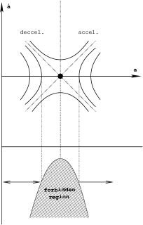
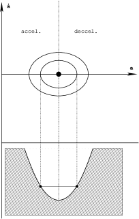
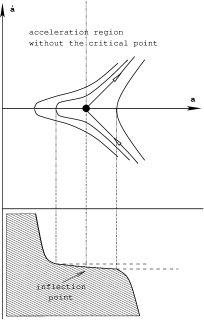
Figure 1: Three types of behavior in the neighborhood of a critical point: a saddle, a center and a cusp.

It is a simple consequence of the fact that characteristic equation for the linearization matrix at the critical point $(\mathop{\text{tr}}{A}=0)$ is $\lambda^{2}+\det{A}=0$, where $\det{A}=\partial^{2}V/\partial x^{2}|_{x_{0}}$. Therefore the eigenvalues are real of opposite sign for saddle point, and for centers – if they are non-hyperbolic critical points – purely imaginary and conjugated.

Finally, if the set of all conservative dark energy models has potential function $V(x)$ such that the number of static critical points and cycles is finite and there are no trajectories connecting saddles then $f\in C^{r}(\mathcal{M})$, $r\geq 1$ contains open, dense subset of all smooth vector fields of class $C^{r}$ on the phase space.

In Fig. 2 the phase portrait for the $\Lambda$CDM model is presented on a compactified projective plane by circle at infinity. Of course it is structurally stable. Therefore, following Peixoto theorem, it is generic in the multiverse $\mathcal{M}$ of all dark energy models with $2D$ phase space because such systems form open and dense subsets.

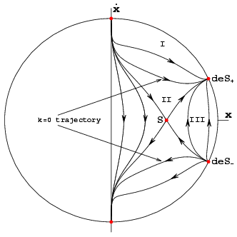
Figure 2: The phase portrait for the $\Lambda$CDM model. On the phase portrait we have a single saddle point in the finite domain and four critical points located on the circle at infinity. They represent initial singularity $(x=0,\dot{x}=\infty)$ or de Sitter Universe deS.
The trajectory of the flat model ($k=0$) divides all models in to two disjoint classes: closed and open. The trajectories situated in the region II confined by the upper branch of the $k=0$ trajectory and by the separatrix going to the stable de Sitter node $\textrm{deS}_{+}$ and by the separatrix going from the initial singularity to the saddle point $S$ correspond to the closed expanding universe. The trajectories located in the regions I and II (which corresponds to the open universes) are called inflectional. Quite similarly, the trajectories situated in the region III correspond to the closed universes contracting from the unstable de Sitter node towards the stable de Sitter node. The trajectories running in this region describe the closed bouncing universes.

It is also interesting that the phase space of dark energy model can be reconstructed from SN Ia data set (Gold Riess sample) and is topologically equivalent to the $\Lambda$CDM model. Fig. 3 represents the potential function

$$V(a(z))=-\frac{1}{2}(1+z)^{2}\Bigg{[}\frac{\mathrm{d}}{\mathrm{d}z}\frac{d_{L}(z)}{1+z}\Bigg{]}^{-2},$$ (9)

reconstructed from $d_{L}(z)$ relation – luminosity distance $d_{L}$ as a function of redshift $z:1+z=a^{-1}$. Such a reconstruction is possible due to the existence of the universal formula

$$\frac{d_{L}(z)}{1+z}=\int\frac{\mathrm{d}z^{\prime}}{H(z^{\prime})},$$ (10)

for the flat model.

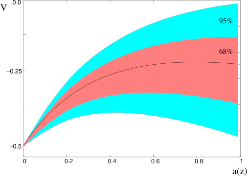
Figure 3: The potential function as a function of the scale factor expressed in its present value $a_{0}=1$ for the reconstructed best fit model is given by the solid line. The confidence regions $1\sigma$ and $2\sigma$ are drawn around it. The phase portrait obtained from this potential (best fit) is equivalent to the $\Lambda$CDM model (see Fig. 2). The value of the redshift transition estimated from SNIa data (the Gold Riess sample) is about $0.38$ (see Czaja et al. (2004)).

In principle it is good news for the $\Lambda$CDM model and others which are close to it in the multiverse in the metric sense.

On the phase portrait the phase space of the Cardassian model is presented (Fig. 4). In the case of single fluid, the presence of additional terms in the modified Friedmann equation is equivalent to extra contribution to the effective energy density in the standard Friedmann equation. On the phase portrait there is a degenerated point $x=\infty,y=0$ located at the infinity.

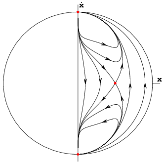
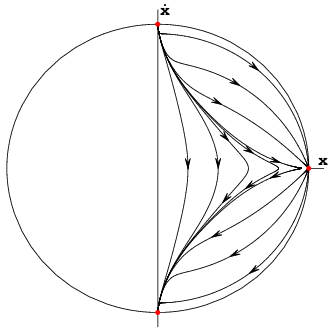
Figure 4: The phase portraits for the Cardassian model $n=-1$ (left) and $n=2$ (right) (see Table 1). The Cardassian model with $n=-1/3$ corresponds to the phantom model with $w_{X}=\textrm{const}<-1$ (generally if we consider dust model equation of state $p_{\textrm{card}}=(n-1)\rho_{\textrm{card}}$ reproduces the Cardassian term).

Let us note that there is no de Sitter attractor at late times. This obstacle was addressed in Ref. Hao and Li (2003); Lazkoz and Leon (2005).

Analogous situation appears if we consider negative value of the exponent $n$ in the Cardassian models. It is well known that if we consider dust matter only Cardassian models with $n<0$ are equivalent to phantom models. The phase portrait for the phantom model ($p_{X}=-(4/3)\rho_{X}$) with dust is illustrated in Fig. 5.

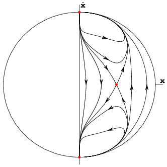
Figure 5: The phase portrait for the phantom model. While at finite domain we find only a saddle point like for the $\Lambda$CDM model, at infinity, the trajectory is reaching the degenerate point $x=0$, $\dot{x}=\infty$. Note that this degeneration can be removed be redefinition of the phase variables and reparameterization of time. Then we obtain other system which is topologically equivalent to the $\Lambda$CDM model (see Fig. 2).

In both cases, Fig. 4 and Fig. 5, the systems are structurally unstable due to the presence of degenerate critical points at infinity. The models with de Sitter phase of evolution at late time are distinguished in the multiverse of dark energy models.

Our main objection addressed to the Cardassian models is that they do not offer description of dark energy epoch in terms of a structurally stable model. Cardassian cosmologies belong to the non-generic, in our terminology, class of fragile model of the present Universe. Similar models form the bifurcation set in the multiverse of dark energy models.

There is also another example of the fragile model used in the cosmological applications – the bouncing model. Such a model recently appeared in the context of semi-classical description of the quantum evolution of the Universe in the framework of loop quantum gravity. In this scenario singularity separates classically allowed regions Ashtekar (2005). The phase portrait of bouncing cosmological model is shown in Fig. 6. In such a cosmology one encounters a bouncing phase of evolution instead of big bang during which the potential function has a minimum. It is structurally unstable due to the presence of non-hyperbolic critical point on the phase portrait. In the next section we find some perturbed system which modifies this and makes it structurally stable.

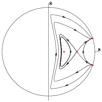
Figure 6: The phase portrait for bouncing (in the contemporary sense see Table 1) cosmological model with $\Lambda$. On the $x$-axis, there are two critical points: center and saddle point. The global phase portrait (in contrast to the $\Lambda$CDM model) is structurally unstable because of the presence of a non-hyperbolic critical point – center. Note that all models (closed, open and flat) undergo a bounce, i.e., they begin their contraction from the unstable de Sitter node, reach a point of minimal contraction and begin expansion toward the stable node $\text{deS}_{+}$.

III Class of dissipative dark energy models

Applying the analogy with pendulum with friction, we would like to incorporate dissipative processes into cosmological model with dark energy. As a matter of fact, dissipative processes should be present in any realistic theory of the Universe Di Prisco et al. (2000).

The simplest way to include bulk viscosity effects is through Eckart’s theory Eckart (1940), which postulates that the bulk viscous pressure is proportional to the expansion. Many authors used that theory to investigate bulk viscosity on the evolution of the Universe Murphy (1973); Belinskii and Khalatnikov (1975).

Basing on Israel and Stewart theory Israel (1976); Israel and Stewart (1979) of truncated viscosity, Belinskii Belinskii et al. (1979) studied effects of viscosity on cosmological models in terms of effective pressure

$$p_{\textrm{eff}}=p-3\xi(\rho)H,$$ (11)

where $p$ is the pressure of a fluid filling the Universe, and $3\xi(\rho)=\bar{\alpha}\rho^{m}$ is the viscosity coefficient parameterized by energy density $\rho=\rho_{\text{eff}}$.

In the context of viscous cosmology many authors used dynamical system methods in investigations of the stationary states and their stability Coley and van den Hoogen (1994). Several authors have studied cosmological models with viscosity Maartens (1996), which are also interesting in the context of inflation de Oliveira and Ramos (1998). It is also interesting that viscosity may describe phenomenologically quantum effects Barrow (1988).

In this section the effects of dissipation are treated as a small perturbation of conservative dark energy models. We then investigate the influence of dissipation on global dynamics of fragile dark energy models.

Let us start with the definition.

Definition 1

A multiverse of the FRW dissipative models with dark energy is defined as a space of all $2$-dimensional perturbed dynamical systems of a Newtonian type

$$\left\{\begin{array}[]{l}\displaystyle{\dot{x}=y},\\ \displaystyle{\dot{y}=-\frac{\partial V}{\partial x}(x)+\bar{\alpha}\rho^{m}(x,y)y}.\end{array}\right.$$ (12)

We have used Belinskii parameterization of the viscosity $3\xi(\rho)=\bar{\alpha}\rho^{m}$ and the first integral $\rho-3H^{2}=3k/x^{2}$ or $\rho_{\text{eff}}=3H^{2}$ is preserved also in the case of viscous cosmology. If $\bar{\alpha}=0$ we obtain the standard conservative FRW cosmology.

It is useful to distinguish two special cases.

III.1 Flat models (k=0)

In this case the dynamical effects of viscosity are equivalent to the effects of Chaplygin gas Fabris et al. (2006); Szydlowski et al. (2006). If we put $p_{\text{eff}}=\gamma\rho-3\alpha\rho^{m}H$ then from the conservation condition $\dot{\rho}=-3H(\rho+p_{\textrm{eff}})$ we obtain the relation

$$\rho(x)=\Bigg{(}\frac{A}{1+\gamma}+\frac{B}{x^{3(1+\gamma)(1+\alpha)}}\Bigg{)}^{\frac{1}{1+\alpha}},$$ (13)

where $A$ and $B$ are integration constants, and $\rho(x=1)=\rho_{0}=\frac{A}{1+\gamma}+B$.

In the special case of $\alpha=0$ $(m=-1/2)$ and $\gamma=0$ (dust) the corresponding equation relating energy density to the scale factor for Chaplygin gas can be recovered. Therefore all the flat models with viscosity following Belinskii parameterization can by represented as conservative systems. To construct the phase space portrait it is useful to represent the potential function $V(x)$ in the similar way as for generalized Chaplygin gas for which the equation of state assumes the following form

$$p=-\frac{A}{\rho^{\alpha}},$$

and energy density can be parameterized by $\rho_{0}$ and $A_{s}$

$$\rho(x)=\rho_{0}\Bigg{(}A_{s}+\frac{1-A_{s}}{x^{3(1+\gamma)(1+\alpha)}}\Bigg{)}^{\frac{1}{1+\alpha}},$$ (14)

where $c^{2}_{s}=\alpha A_{s}$ is the squared velocity of sound. Therefore the potential function for the system is given by

$$V(x)=-\frac{\rho x^{2}}{6}=-\frac{1}{2}\Omega_{\text{visc},0}x^{2}\Bigg{(}A_{s}+\frac{1-A_{s}}{x^{3(1+\gamma)(1+\alpha)}}\Bigg{)}^{\frac{1}{1+\alpha}},$$ (15)

where $1+\alpha=1/2-m$, $A_{s}=\frac{A}{1+\gamma}$, $\Omega_{\text{visc},0}=\frac{\rho_{0}}{3H_{0}^{2}}$.

In Figs. 7 and  8 the phase portraits for different parameter $m$ and for different equation of state coefficient $\gamma$ are illustrated. Therefore the effect of viscosity in the perfect fluid is equivalent to the effect of Chaplygin gas in the case of flat model.

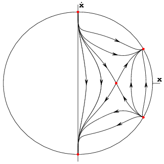
a) b)

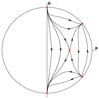
c)

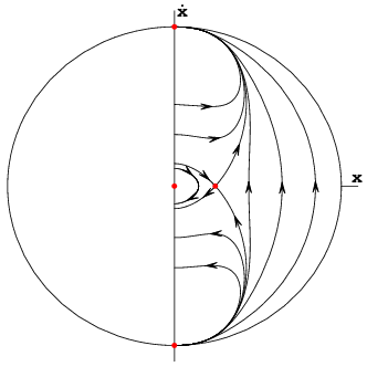
Figure 7: The phase portraits for the viscous cosmological models. a) $\gamma=0$, $\alpha=0$ ($m=-1/2$), $A_{s}=0.3$, b) $\gamma=1/3$, $\alpha=1/2$ ($m=-1$), $A_{s}=0.5$, c) $\gamma=-4/3$, $\alpha=0$ ($m=-1/2$), $A_{s}=-0.95$. Note that both models presented in Fig. a) and b) are topologically equivalent.

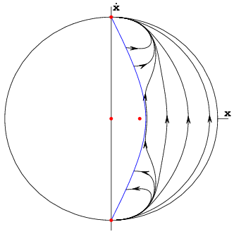
d) e)

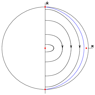
Figure 8: The phase portraits for the viscous cosmological models. d) $\gamma=-4/3$, $\alpha=1/2$ ($m=-1$), $A_{s}=-0.5$, and the solid (blue in el. version) line denotes the limit $x=x_{\textrm{min}}$, e) $\gamma=-4/3$, $\alpha=-3/2$ ($m=1$), $A_{s}=-0.5$, the solid line denotes the limit $x=x_{\textrm{max}}$.

Note that for phantom cosmology ($\gamma<-1$) $A_{s}$ can be either negative or positive but if $A_{s}$ is negative, the expression in the parentheses should be positive. Therefore we obtain following inequalities which restrict $x=x_{\textrm{min}}$ or $x=x_{\textrm{max}}$

$$x=\left\{\begin{array}[]{lcl}<\big{(}\frac{A_{s}-1}{A_{s}}\big{)}^{\frac{1}{3(1+\gamma)(1+\alpha)}}&\textrm{if}&(1+\gamma)(1+\alpha)>0,\\ >\big{(}\frac{A_{s}-1}{A_{s}}\big{)}^{\frac{1}{3(1+\gamma)(1+\alpha)}}&\textrm{if}&(1+\gamma)(1+\alpha)<0.\\ \end{array}\right.$$

Therefore for $A_{s}<0$ ($1+\gamma<0$) $x<x_{\textrm{max}}$ if only $\alpha<-1$ ($m>1/2$) and $x>x_{\textrm{min}}$ if only $\alpha>-1$ ($m<1/2$).

If we assume that $\gamma>-1$, then the Chaplygin gas interpolates between the state of positive cosmological constant and state of matter domination $\rho\propto a^{-3(1+\gamma)}$ at the early epoch. Hence the viscosity effects can shift structurally unstable model into open dense set. Fig. 9 shows the influence of viscosity on bouncing models for which the potential function contains additional contribution which can unify matter $(p=0)$ and dark energy.

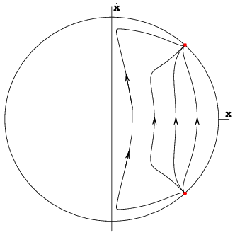
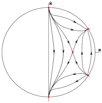
Figure 9: The bouncing models with viscosity for potential (16) with $A_{s}=0.75$. $\Omega_{\text{visc},0}>1$ (left) and $\Omega_{\text{visc},0}<1$ (right). Note that viscosity makes the global phase portraits of bouncing models structurally stable.

If we postulate the existence of negative contribution to the effective energy density coming, for example, from quantum effects like in Vandersloot’s approach Vandersloot (2005); Singh and Vandersloot (2005), then the potential function assumes the following form

$$V(x)=-\frac{1}{2}\Bigg{\{}\Omega_{\text{visc},0}x^{2}\bigg{(}A_{s}+\frac{1-A_{s}}{x^{3(\frac{1}{2}-m)}}\bigg{)}^{\frac{1}{\frac{1}{2}-m}}-\frac{1}{2}\Omega_{lq,0}x^{-4}\Bigg{\}}.$$ (16)

where $\Omega_{\text{visc},0}-\Omega_{lq,0}=1$ and then the cosmological model exhibits characteristic bounce phase Hossain (2005); Szydłowski et al. (2005).

It is characteristic for loop quantum cosmology that initial singularity is replaced with bounce because of quantum effects which are manifested by presence of negative energy contribution to the $H^{2}(a)$ relation. In this picture space-time does not end at singularities and quantum regime can offer a bridge between vast space-time regions which are classically unrelated (see Ashtekar (2005)).

Unfortunately, in the phase space we obtain a non-hyperbolic critical point around the bounce which makes the system structurally unstable. In Fig. 9 it is illustrated how small viscosity effects (or equivalently the Chaplygin gas) can dramatically change global phase portraits and makes the corresponding system (with potential (16)) structurally stable.

III.2 Case of constant viscosity (m=0)

Let us start now the analysis of the effects of viscosity in the case of constant viscosity. In this special case the equation of motion assumes a very simple form

$$\left\{\begin{array}[]{l}\displaystyle{\dot{x}=y},\\ \displaystyle{\dot{y}=-\frac{\partial V}{\partial x}(x)+\alpha y}.\end{array}\right.$$ (17)

One can calculate the distance from a dissipative system (17) to a conservative one. Then the perturbation vector is

$$\delta=[0,\alpha y]^{T},$$

and distance

$$d(cons,dissip)=\max_{(x,y)\in E}\big{\{}|\alpha y|,\alpha\big{\}}=\alpha\max_{(x,y)\in E}\big{\{}|y|,1\big{\}},$$

where $E$ is a compact region of the phase space in which we compare models, which we chose as the region $|y|<1$. Hence the parameter $\alpha$ will measure the distance from a viscous perturbed system to a conservative system, in $C^{1}$ metric. It is interesting that the exact solution of the system (17) with constant viscosity can be simply obtained, without any assumption about the curvature, if we know the corresponding solution without the viscosity. The following theorem establishes this fact.

Theorem 1

Let $t=\phi(a)$ be a solution of the conservative system with dark energy

$$\dot{a}=(-2V(a))^{-1/2}.$$

It can be determined from the relation

$$t(a)=\int^{a}\frac{\mathrm{d}x}{\sqrt{-2V(x)}}=\phi(a).$$

Then solution of the type

$$\exp{[\alpha t]}=\phi(a),$$ (18)

will be the solution with constant viscosity $\alpha$.

To prove this fact, it is sufficient to check that solution of the above type will satisfy equation

$$\ddot{a}=-\frac{\partial V}{\partial a}+\alpha\dot{a},$$

which is equivalent to equation (17).

One can consider now the properties of the phase plane of the dissipative dark energy models. We are especially interested whether bouncing models can be shifted to the generic set of the multiverse.

The location of all critical points at finite domain coincides with that of the case without dissipation effects because all should be situated on the $x$–axis (static critical point). Their character is determined by the linearization matrix

$$A=\left[\begin{array}[]{cc}0&1\\ \displaystyle{-\frac{\partial^{2}V}{\partial x^{2}}}&\alpha\end{array}\right]_{(x_{0},0)}.$$ (19)

Because $\mathop{\text{tr}}{A}=\alpha>0$ all the critical points are unstable. The characteristic equation assumes the following form

$$\lambda^{2}-\alpha\lambda+V_{xx}(x_{0})=0.$$ (20)

Therefore the eigenvalues of the linearization matrix (19) are real of the same signs if $V_{xx}(x_{0})>0$ and opposite signs if $\lambda_{1}\lambda_{2}=V_{xx}(x_{0})<0$. They are real if $\Delta=\alpha^{2}-4V_{xx}(x_{0})$ is positive, or imaginary if $\Delta$ is negative. In any case $\mathop{\text{Re}}{\lambda}=\alpha$ is different from zero, i.e., all critical points are hyperbolic. Note that if $V_{xx}(x_{0})<0$ then always $\Delta>0$, i.e., eigenvalues are real of opposite signs (they are representing saddles). If $V_{xx}(x_{0})>0$ (like in the neighborhood of bounce) then eigenvalues are real and positive ($\lambda_{1}+\lambda_{2}=\alpha$ and $\lambda_{1}\lambda_{2}>0$) or imaginary (if $V_{xx}(x_{0})>\alpha^{2}/4$). This corresponds to the presence of an unstable node or an unstable focus on phase portraits, respectively. Because both unstable nodes are topologically equivalent to the unstable focus, we obtain generic phase portraits for the dissipative bouncing model which are demonstrated in Fig. 10.

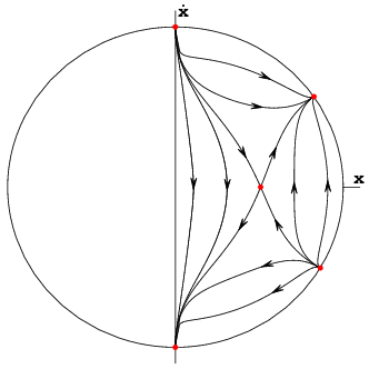
a) b)

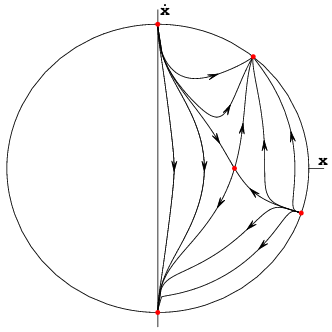
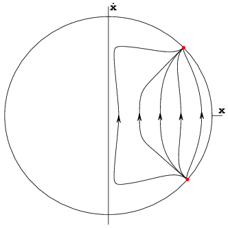
c) d)

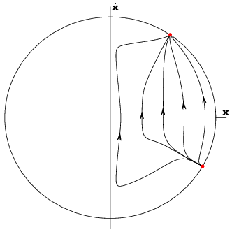
Figure 10: The phase portrait of the system (23) for the bouncing $\Lambda$CDM model with a constant viscosity coefficient which assumes different values. Cases: a) $\Omega_{\Lambda,0}=0.4$, $\Omega_{\text{m},0}=0.3$, $\alpha=0.1$, b) the same but with $\alpha=0.9$; c) $\Omega_{\Lambda,0}=0.8$, $\Omega_{\text{m},0}=0.3$, $\alpha=0.1$, d) the same as previous but with $\alpha=0.9$. Note that all phase portraits are structurally stable due to viscosity perturbation and that symmetry $\dot{x}\to-\dot{x}$ can be broken if viscosity effects are included. It is because entropy is changing due to the presence of dissipative processes.

Let us now present some general properties of the dissipative FRW models. The equation of motion is in the form

$$\left\{\begin{array}[]{l}\displaystyle{\dot{x}=y\equiv P(x,y)},\\ \displaystyle{\dot{y}=-\frac{\partial V}{\partial x}(x)+\alpha y\equiv Q(x,y)}.\end{array}\right.$$ (21)

The critical points at finite domain (only repellors) are determined from

$$y_{0}=0,\qquad\bigg{(}\frac{\partial V}{\partial x}\bigg{)}_{x_{0}}=0.$$

System (21) linearized around the static critical point $(x_{0},0)$ has the form

$$\left\{\begin{array}[]{l}\displaystyle{(x-x_{0})\dot{}=\bigg{(}\frac{\partial P}{\partial x}\bigg{)}_{(x_{0},0)}(x-x_{0})+\bigg{(}\frac{\partial P}{\partial y}\bigg{)}_{(x_{0},0)}(y-y_{0})},\\ \displaystyle{(y-y_{0})\dot{}=\bigg{(}\frac{\partial Q}{\partial x}\bigg{)}_{(x_{0},0)}(x-x_{0})+\bigg{(}\frac{\partial Q}{\partial y}\bigg{)}_{(x_{0},0)}(y-y_{0})},\end{array}\right.$$

or

$$\left\{\begin{array}[]{l}\displaystyle{\dot{x}=y},\\ \displaystyle{\dot{y}=-\bigg{(}\frac{\partial^{2}V}{\partial x^{2}}\bigg{)}_{(x_{0},0)}(x-x_{0})}.\end{array}\right.$$

It is useful to shift the critical point to the origin of a new coordinate system labelled as $(X,Y)$, say $x\to X=x-x_{0}$, $Y=y$. Then

$$\left\{\begin{array}[]{l}\displaystyle{\dot{X}=Y},\\ \displaystyle{\dot{Y}=-\bigg{(}\frac{\partial^{2}V}{\partial X^{2}}\bigg{)}_{(0,0)}X},\end{array}\right.$$

or $\dot{\boldsymbol{X}}=A\boldsymbol{X}$. Let us consider the special case of a conservative system for $\alpha=0$. The solutions of the system are

$$X=C_{1}\exp{[\lambda_{1}t]}+C_{2}\exp{[\lambda_{2}t]},$$

where $C_{1}$ and $C_{2}$ are constants and $\lambda_{1}$, $\lambda_{2}$ are eigenvalues of the linearization matrix.

There are two types of the solutions:

1. solution of a saddle point if eigenvalues are real of opposite signs $\lambda_{1,2}=\pm\sqrt{-\det{A}}=\pm\sqrt{-\big{(}\frac{\partial^{2}V}{\partial X^{2}}\big{)}_{(0,0)}}$,

2. solution of a center type when eigenvalues are imaginary $\lambda_{1,2}=\pm i\sqrt{-\det{A}}=\pm i\sqrt{\big{(}\frac{\partial^{2}V}{\partial X^{2}}\big{)}_{(0,0)}}$.

Finally we obtain corresponding solution

$$x-x_{0}=C_{1}\exp{[\sqrt{\bigg{(}-\frac{\partial^{2}V}{\partial x^{2}}\bigg{)}_{x=x_{0}}}t]}+C_{2}\exp{[-\sqrt{\bigg{(}-\frac{\partial^{2}V}{\partial x^{2}}\bigg{)}_{x=x_{0}}}t]},$$

or

$$x-x_{0}=C_{1}\cos{\sqrt{\bigg{(}\frac{\partial^{2}V}{\partial x^{2}}\bigg{)}_{x=x_{0}}}t}+C_{2}\sin{\sqrt{\bigg{(}\frac{\partial^{2}V}{\partial x^{2}}\bigg{)}_{x=x_{0}}}t}.$$

In the case of dissipative ($\alpha=$ const) dynamical system the characteristic equation assumes the form (20) and solutions are $\lambda_{1,2}=-\frac{\alpha\pm\sqrt{\Delta}}{2}$ and $\lambda_{1}\lambda_{2}=\det{A}=\big{(}\frac{\partial^{2}V}{\partial x^{2}}\big{)}_{x_{0}}$. In this case the type of the critical points (if they exist) will depend on both the sign of discriminant $\Delta=\alpha^{2}-4V_{xx}(x_{0})$ and sign of $V_{xx}(x_{0})$ at the critical points, namely

• if $V_{xx}(x_{0})<0$, i.e. $V(x)$ has a maximum then critical points are always saddles,

• if $V_{xx}(x_{0})>0$, i.e. $V(x)$ has a minimum at $x_{0}$ then character of the critical points will depend on the value of $\alpha$ such that:

  • if $\alpha>2\sqrt{V_{xx}(x_{0})}$ then we have unstable nodes,

  • if $0<\alpha<2\sqrt{V_{xx}(x_{0})}$ then we obtain unstable focus.

Therefore in $\alpha$ is sufficiently small then unstable focus is present on the phase portrait instead of center in the conservative case. If $\alpha$ is sufficiently large then we obtain unstable node at the minimum of the diagram of the potential function. Note that except of degeneration case of center all admissible critical points are structurally stable. The focus is topologically equivalent to node.

Note that the presence of dissipative effects enlarge the accelerating domain occupied by accelerating cosmological models because of relation

$$-\frac{\partial V}{\partial x}(x)+\alpha y>0,$$ (22)

and now this region depends additionally on the coordinate $y$. Note that at the critical point relation (22) is always valid (like in Vandersloot (2005)).

If we substitute in (17) the form of the potential function for bouncing cosmology with $\gamma=0$ (dust) and $n=4$, then the corresponding dynamical system has the form

$$\left\{\begin{array}[]{l}\displaystyle{\dot{x}=y},\\ \displaystyle{\dot{y}=-\frac{1}{2}\Omega_{\text{m},0}x^{-2}+\Omega_{n,0}x^{-3}+\Omega_{\Lambda,0}x+\alpha y}.\end{array}\right.$$ (23)

Rescaling the time variable we can make r.h.s. of the system (23) polynomial. The simple time transformation given by $\tau\mapsto\eta\colon\mathrm{d}\tau/x^{3}=\mathrm{d}\eta$ give rise to its regularization. Such a choice of new time variable does not change the phase portrait because our system has been autonomous since the very beginning. This operation is equivalent to multiplication of the r.h.s. by $x^{3}$ so that the system can be considered in the $\eta$ time, because $x>0$ and $\eta$ is a monotonous function of any time $\tau$. Finally we obtain

$$\left\{\begin{array}[]{l}\displaystyle{\frac{\mathrm{d}x}{\mathrm{d}\eta}=yx^{3}},\\ \displaystyle{\frac{\mathrm{d}y}{\mathrm{d}\eta}=-\frac{1}{2}\Omega_{\text{m},0}x+\Omega_{n,0}+\Omega_{\Lambda,0}x^{4}+\alpha yx^{3}},\end{array}\right.$$ (24)

where $\Omega_{\text{m},0}-\Omega_{n,0}+\Omega_{\Lambda,0}=1$.

Note that reparameterization of cosmological time is equivalent to the choice of the corresponding lapse function $N(t)$ in such a way that $\tau=\int N(t)\mathrm{d}t$. If we consider particle like representation of the dynamics then we obtain classical mechanics with lapse in the H.-J. Schmidt terminology Schmidt (1996).

The degeneration of the dynamics at infinity for phantoms can be removed in a simple way by introducing a new positional variable $\bar{x}$ such that

$$x\mapsto\bar{x}=x^{\frac{3}{2}}$$

(in general $\bar{x}=x^{-(1+3w)/2}$) and reparameterizing the time variable

$$\begin{array}[]{rl}\tau\mapsto\eta\colon&\frac{3}{2}\bar{x}^{\frac{1}{3}}\mathrm{d}t=\mathrm{d}\eta,\\ \textrm{or}:&\frac{3}{2}x^{\frac{1}{2}}\mathrm{d}t=\mathrm{d}\eta.\end{array}$$

Of course the new time variable is a monotonous function of the original time $\tau$. Hence we obtain the new system in which the original variable $y$ preserves its original sense

$$\left\{\begin{array}[]{l}\displaystyle{\frac{\mathrm{d}\bar{x}}{\mathrm{d}\eta}=y},\\ \displaystyle{\frac{\mathrm{d}y}{\mathrm{d}\eta}=-\frac{1}{3}\left(-\Omega_{\text{m},0}\bar{x}^{-\frac{5}{3}}+3\Omega_{\text{ph}}\bar{x}\right)=-\frac{\partial V}{\partial\bar{x}}}.\end{array}\right.$$

New potential function assumes the form

$$V(\bar{x})=-\frac{1}{2}\bigg{\{}\Omega_{\text{m},0}\bar{x}^{-\frac{2}{3}}+\Omega_{\text{ph}}\bar{x}^{2}+\Omega_{k,0}\bigg{\}}.$$

The above system is of Newtonian type and has a first integral in the energy conservation form

$$\frac{y^{2}}{2}+V(\bar{x})=0,$$

where now $y=\frac{\mathrm{d}\bar{x}}{\mathrm{d}\eta}$.

It is easy to check that the kinetic energy form $\frac{1}{2}(\frac{\mathrm{d}\bar{x}}{\mathrm{d}\eta})^{2}=\frac{1}{2}(\frac{\mathrm{d}x}{\mathrm{d}t})^{2}$ is preserved under nonlinear rescaling transformation $x\mapsto\bar{x}$ and time reparameterization. The form of the potential function $V(\bar{x})$ is de facto the same as the original $V(x)$ in which instead of $x$ we operate on $\bar{x}$ as the positional variable.

From the first integral we obtain that for large $\bar{x}$ we have

$$\frac{y}{\bar{x}}=\sqrt{\Omega_{ph}}$$

because material contribution is negligible. It means that asymptotically the trajectories reach the point which lies on the circle at infinity and on the straight line $y\propto\bar{x}$. The corresponding dynamical system on the plane $(\bar{x},y)$ is of course equivalent to the $\Lambda$CDM model phase portrait although we must remember that the attractor at infinity does not represent the de Sitter universe. Therefore the obtained global phase portrait for phantom cosmology is structurally stable in a similar way as in the case of the $\Lambda$CDM model.

The analogous “regularization procedure” which we perform for phantom with $w=-\frac{4}{3}$ can be realized in a more general case for any $w$. It is sufficient to choose

$$\begin{array}[]{rl}x\mapsto\bar{x}\colon&\bar{x}=x^{-\frac{1+3w}{2}},\\ \tau\mapsto\eta\colon&\mathrm{d}\eta=-(\frac{1+3w}{2})x^{-\frac{3}{2}(1+w)}\mathrm{d}t.\\ \end{array}$$

The corresponding potential function is

$$V(\bar{x})=-\frac{1}{2}\bigg{\{}\Omega_{\text{m},0}\bar{x}^{-\frac{2}{3}}+\Omega_{w,0}\bar{x}^{2}+\Omega_{k,0}\bigg{\}}.$$

Therefore phantom cosmology in which a weak energy condition is violated forms an open and dense subsets in the multiverse of all dark energy models. Also big-rip singularities which are attributed to these classes of models are a generic features of their long term behavior.

The universe is accelerating in the region of phase space determined by the condition

$$-\Omega_{\text{m},0}x+2\bigg{\{}\Omega_{n,0}+\Omega_{\Lambda,0}x^{4}+\alpha yx^{3}\bigg{\}}>0,$$ (25)

and finally region of accelerating expansion is given by

$$y>\frac{1}{\alpha x^{3}}\bigg{\{}\frac{1}{2}\Omega_{\text{m},0}x-\Omega_{n,0}-\Omega_{\Lambda,0}x^{4}\bigg{\}}$$

Therefore all terms apart from the matter term $\Omega_{\text{m},0}$ act toward the acceleration of the Universe.

IV Viscous cosmology tested by distant supernovae type Ia

Using the energy conservation condition we can obtain a simple relation

$$\rho(a)=\bigg{[}\frac{A}{1+\gamma}+\frac{B}{a^{3(1+\gamma)(\frac{1}{2}-m)}}\bigg{]}^{\frac{1}{\frac{1}{2}-m}},$$

where $A=3\alpha$ is a positive constant which quantifies if viscous effects appeared, $B$ is an arbitrary integration constant. For small value of the scale factor $a(t)$ we have

$$\rho(a)\simeq\frac{B^{{1}/{(\frac{1}{2}-m)}}}{a^{3(1+\gamma)}},$$

which corresponds to the universe dominated by matter satisfying equation of state $p=\gamma\rho$. Also for a large value of scale factor (if $1+\gamma>0$)

$$\rho\simeq\bigg{(}\frac{A}{1+\gamma}\bigg{)}^{\frac{1}{\frac{1}{2}-m}}\qquad\textrm{and}\qquad p\simeq-\bigg{(}\frac{A}{1+\gamma}\bigg{)}^{\frac{1}{\frac{1}{2}-m}}=-\rho,$$

which corresponds to an otherwise empty universe with cosmological constant $\big{(}\frac{A}{1+\gamma}\big{)}^{{1}/{(\frac{1}{2}-m)}}$. For an accelerating universe, the deceleration parameter must be negative, therefore

$$a^{3(1+\gamma)(\frac{1}{2}-m)}>\frac{B(1+\gamma)(1+3\gamma)}{3A}.$$

The above expression indicates that if $(\frac{1}{2}-m)(1+\gamma)>0$ then a universe starts to accelerate when the scale factor is reaching its critical value

$$a_{\text{trans}}=\bigg{[}\frac{B(1+\gamma)(1+3\gamma)}{2A}\bigg{]}^{\frac{1}{3({1}/{2}-m)(1+\gamma)}}.$$

Hence the interpolation of early matter domination phase and cosmological constant epoch is achieved for viscous fluid when the viscosity decreases when density is decreasing. If we put $a=1$ at the present epoch then present Universe is accelerating if $\big{(}\frac{B}{A}\big{)}(1+\gamma)(1+3\gamma)<1$.

An important test allows to verify if the viscosity fluid may represent dark energy is the comparison with the supernovae type Ia data. For this purpose we have to calculate the luminosity distance in the model

$$d_{L}(z)=(1+z)\frac{c}{H_{0}}\int_{0}^{z}\frac{\mathrm{d}z^{\prime}}{H(z^{\prime})}.$$ (26)

The Friedman equation can be rearranged to the form giving explicitly the Hubble function $H(z)={\dot{a}}/a$

$$H(z)^{2}=H_{0}^{2}\left[\Omega_{\text{m}}(1+z)^{3}+\Omega_{\text{visc}}\left(A_{s}+(1-A_{s})(1+z)^{3(1+\alpha)}\right)^{\frac{1}{1+\alpha}}\right]$$ (27)

where the quantities $\Omega_{i}$, $i=\text{m},\text{visc},k$ represent fractions of critical density currently contained in energy densities of respective components and $\Omega_{\text{m}}+\Omega_{\text{visc}}+\Omega_{k}=1$.

This model adds to our previous discussion of a viscous fluid the additional elements of curvature and matter scaling like dust. As discussed above (see equation (13)), the viscous fluid has a Chaplygin-like dependence on scale factor only in the flat dust-free case; in other circumstances, equation (27) does not represent the solution for a universe containing in part a viscous fluid. Therefore, this model is in general to be regarded as an empirical construct. Such a model can nevertheless be compared to data, and we do this below; where we mention model testing, we actually mean the estimation of the $m$ and $A_{s}$ parameters for the best fit FRW cosmological model. We will mostly use the flat model $k=0$ (the exception takes place when we relax a flat prior) since the evidence of this case is very strong in the light of current CMBR data.

Formula (28) is the most general one in the framework of the Friedmann-Robertson-Walker models with this unified macroscopic (phenomenological) description of both dark energy and dark matter (quartessence). We assume that $\Omega_{\text{m,0}}=\Omega_{\text{b},0}$

Finally the luminosity distance reads

$$d_{L}(z)=(1+z)\frac{c}{H_{0}}\int_{0}^{z}\frac{\mathrm{d}z^{\prime}}{\sqrt{\Omega_{\text{m},0}(1+z)^{3}+\Omega_{\text{visc},0}\left(A_{s}+(1-A_{s})(1+z)^{3(1+\alpha)}\right)^{\frac{1}{1+\alpha}}}}.$$ (28)

To proceed with fitting the SNIa data we need the magnitude-redshift relation

$$m(z,{\cal M},\Omega_{\text{m},0},\Omega_{\text{visc},0};A_{s},\alpha)={\cal M}+5\log_{10}D_{L}(z,\Omega_{\text{m},0},\Omega_{\text{visc},0};A_{s},\alpha)$$ (29)

where:

$$D_{L}(z,\Omega_{\text{m},0},\Omega_{\text{visc},0};A_{s},\alpha)=H_{0}d_{L}(z,H_{0},\Omega_{\text{m},0},\Omega_{\text{Ch},0};A_{s},\alpha)$$

is the luminosity distance with $H_{0}$ factored out so that marginalization over the intercept

$${\cal M}=M-5\log_{10}H_{0}+25$$ (30)

leads actually to joint marginalization over $H_{0}$ and $M$ ($M$ being the absolute magnitude of SNIa).

Then we can obtain the best fitted model minimizing the $\chi^{2}$ function

$$\chi^{2}=\sum_{i}\frac{(m_{i}^{Ch}-m_{i}^{obs})^{2}}{\sigma_{i}^{2}}$$

where the sum is over the SNIa sample and $\sigma_{i}$ denote the (full) statistical error of magnitude determination. This is illustrated in Fig. 11 of residuals (with respect to the Einstein-de Sitter model) and $\chi^{2}$ levels in the $(A_{s},m)$ plane. One of the advantages of residual plots is that the intercept of the $m-z$ curve gets cancelled. The assumption that the intercept is the same for different cosmological models is legitimate since ${\cal M}$ is actually determined from the low-redshift part of the Hubble diagram which should be linear in all realistic cosmologies.

The best fit values alone are not relevant if not supplemented with the confidence levels for the parameters. Therefore, we performed the estimation of model parameters using the minimization procedure, based on the likelihood function. We assumed that supernovae measurements came with uncorrelated Gaussian errors and in this case the likelihood function ${\cal L}$ could be determined from chi-square statistic ${\cal L}\propto\exp{(-\chi^{2}/2)}$ Riess et al. (1998); Perlmutter et al. (1999).

Therefore we supplement our analysis with confidence intervals in the $(A_{s},m)$ plane by calculating the marginal probability density functions

$${\cal P}(A_{s},\alpha)\propto\int\exp{\bigg{(}-\frac{1}{2}\chi^{2}(\Omega_{\text{m},0},\Omega_{\text{visc},0},A_{s},\alpha,{\cal M})\bigg{)}}\mathrm{d}{\cal M}$$

with $\Omega_{\text{m},0},\Omega_{\text{visc},0}$ fixed ($\Omega_{\text{m},0}=0.0,0.05,0.3$) and

$${\cal P}(A_{s},\alpha)\propto\int\exp{\bigg{(}-\frac{1}{2}\chi^{2}(\Omega_{\text{m},0},\Omega_{\text{visc},0},A_{s},\alpha,{\cal M})\bigg{)}}\mathrm{d}{\Omega_{\text{m},0}}$$

with ${\cal M}$ fixed (${\cal M}=-3.39$) respectively (a proportionality sign means equal up to the normalization constant) (Fig.12). In order to complete the picture we have also derived one-dimensional probability distribution functions for $\Omega_{\text{visc}}$ obtained from joint marginalization over $m$ and $A_{s}$. The maximum value of such PDF informs us about the most probable value of $\Omega_{\text{visc},0}$ (supported by supernovae data) within the full class of viscous cosmological models.

Adopting an analogy to the models with generalized Chaplygin gas (GCG) one can see that $\rho_{\text{visc},0}=\big{(}\frac{A}{1+\gamma}+B\big{)}^{\frac{1}{1/2-m}}$ represents the current energy density of the viscous fluid for which one can define density parameters in the standard way. One can also calculate the adiabatic speed of sound squared for viscous fluid

$$c_{s}^{2}=\frac{(-\frac{1}{2}-m)\frac{A}{1+\gamma}}{\frac{A}{1+\gamma}+\frac{B}{a^{3(1/2-m)}}}.$$

Therefore $c_{s,0}^{2}=\frac{\alpha\frac{A}{1+\gamma}}{\frac{A}{1+\gamma}+B}$ (velocity of light at present epoch) and constants $A$ and $B$ can be expressed in terms of quantities having well defined physical meaning. Instead of constants $A$ and $B$ it is useful to consider new ones $A_{s}=\frac{A}{1+\gamma}$, $B=1-A_{s}$ and $\rho_{\text{visc},0}$. Then $c_{s,0}^{2}=(-\frac{1}{2}-m)A_{s}$ in the units of the speed of light $c$.

Figure 11: Results from the Gold sample. Residuals (in mag) between the Einstein-de Sitter model (zero line), and three flat models: with $m=0$, the flat $\Lambda$CDM model ($m=-0.5$), and $m=-1.5$ (equivalent to Chaplygin gas model with $\alpha=1$). Note that in the viscous cosmology distant $z>1$ supernovae should be brighter than in the $\Lambda$CDM model. Therefore future distant supernovae data can definitely distinguish: which cosmology, with dark energy with dissipation or not?

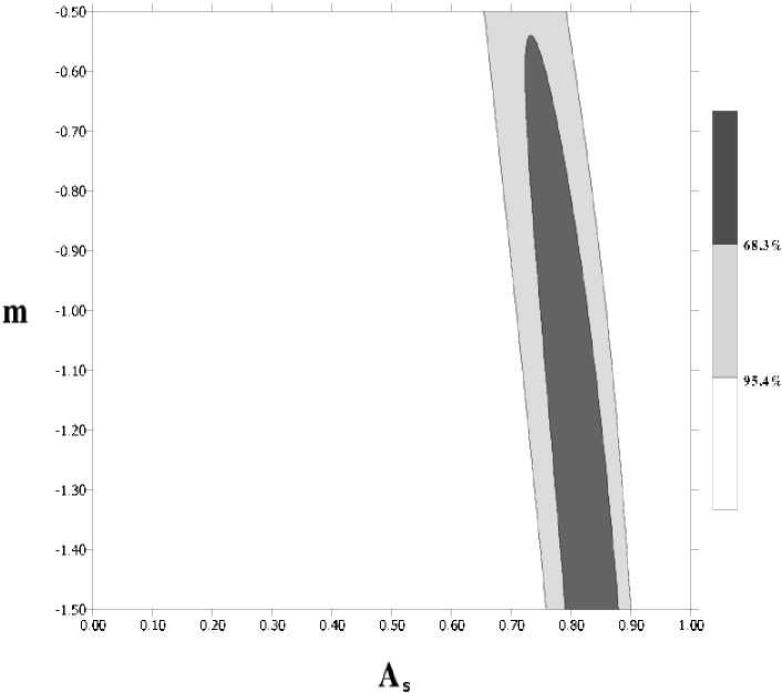
Figure 12: Confidence levels on the $(A_{s},m)$ plane for the viscous cosmological model, marginalized over ${\cal M}$, and $\Omega_{\text{m},0}$.

IV.1 Fits to $A_{s}$ and $m$ parameters

IV.1.1 Samples used

We use data sets which were compiled by Riess et al. Riess et al. (2004), they have been used by many researchers as a standard dataset. They improved the former Riess et al. sample and discovered 16 new type Ia supernovae. It should be noted that 6 of these objects have $z>1.25$ (out of total number of 7 object with so high red shifts). Moreover, they compiled a set of previously observed SNIa relying on large, published samples, whenever possible, to reduce systematic errors from differences in calibrations. Thanks to this enriched sample it became possible to test our prediction that distant supernovae should be brighter in viscous cosmology than in the $\Lambda$CDM model (see discussion below).

The full Riess sample contains 186 SNIa (“Silver” sample). Taking into account the quality of the spectroscopic and photometric record for individual supernovae, they also selected a more restricted “Gold” sample of 157 supernovae. We have separately analyzed the $\Lambda$CDM model for supernovae with $z<1$ and for all SNIa belonging to the Gold sample.

IV.1.2 Viscous cosmological models tested

Using these samples we have tested viscous cosmology in three different classes of models with (1) $\Omega_{\text{m},0}=0.3$, $\Omega_{\text{visc},0}=0.7$; (2) $\Omega_{\text{m},0}=0.05$, $\Omega_{\text{visc},0}=0.95$ and (3) $\Omega_{\text{m},0}=0$, $\Omega_{\text{visc},0}=1$. We started with a fixed value of ${\cal M}=-3.39$ modifying this assumption accordingly while analyzing different samples.

The first class was chosen as representative of the standard knowledge of $\Omega_{\text{m},0}$ (baryonic plus dark matter in galactic halos Peebles and Ratra (2003)) with viscosity responsible for the missing part of closure density (the dark energy).

In the second class we have incorporated (at the level of $\Omega_{\text{m},0}$) the prior knowledge about the baryonic content of the Universe (as inferred from the BBN considerations). Hence this class is representative of the models in which the viscous fluid is allowed to clump and is responsible both for dark matter in halos as well as its diffuse part (dark energy).

The third class is a kind of toy model – the FRW universe filled completely with viscous fluid. We have considered it mainly in order to see how sensitive the SNIa test is with respect to parameters identifying the cosmological model.

Finally, we analyzed the data without any prior assumption about $\Omega_{\text{m},0}$.

IV.1.3 Results

For statistical analysis we restricted the values of the $A_{s}$ parameter $[0,1.0]$ and $m$ to the interval $[-0.5,-1.5]$ because of the relation $c_{s}^{2}=\alpha\,A_{s}$ (where $\alpha=-0.5-m$). This constraint guarantee that in all cases $c_{s}$ is real and does not exceed $c=1$. We separately analyze the case of $m=0$, which corresponds to constant viscosity coefficient.

The results (best fits) of two fitting procedures performed on Riess samples and with different prior assumptions concerning the cosmological models are presented in Tables 2 and 3. Table 2 refers to the $\chi^{2}$ method whereas in Table 3 the results from marginalized probability density functions is displayed. In both cases we obtained different values of ${\cal M}$ for each analyzed sample. In Table 4 we gather results of the statistical analysis of the viscous cosmological model performed on the Gold Riess sample of SNIa as a minimum $\chi^{2}$ best fit for different values of fixed $m$.

First, we present residual plots of redshift-magnitude relations between the Einstein-de Sitter model (represented by zero line) and models with $m=0$ — upper curve, $m=-0.5$ (this model is equivalent to the $\Lambda$CDM model) — middle curve, and $m=-1.5$ (this model is equivalent to the GCG) — lower curve. One can observe that systematic deviation between these models is larger at higher red-shifts. The viscous model ($m=-1.5$) predicts that high redshift supernovae should be brighter than what is predicted with the $\Lambda$CDM model, while in the model with $m=0$ high redshift supernovae should be fainter than those predicted with the $\Lambda$CDM model.

The Riess sample leads to the results which are similar to these obtained recently with the Astier sample Astier et al. (2006). For the Gold sample, the joint marginalization over parameters gives the following results: $\Omega_{\text{visc},0}=1.00$ (hence $\Omega_{\text{m},0}=0.0$), with the limit $\Omega_{\text{visc},0}\geq 0.80$ at the confidence level of $68.3\%$ and $\Omega_{\text{visc},0}\geq 0.69$ at the confidence level of $95.4\%$. $(m=-1.5,A_{s}=0.83)$ with the interval $m\in(-0.86,-1.5)$ and $A_{s}\in(0.76,0.94)$ at the confidence level of $68.3\%$ and $m\in(-0.55,-1.5)$ and $A_{s}\in(0.72,1.00)$ at the confidence level of $95.4\%$.

IV.2 Information criteria

In the modern observational cosmology the so called degeneracy problem is present: many models with dramatically different scenarios are in good agreement with the present observations. Information criteria of the model selection Liddle (2004) can be used to solve this degeneracy among some subclass of dark energy models. Among these criteria the Akaike information criterion (AIC) Akaike (1974) and the Bayesian information criterion (BIC) Schwarz (1978) are most popular. From these criteria we can determine the number of the essential model parameters providing the preferred fit to the data.

The AIC is defined in the following way Akaike (1974)

$$\mathrm{AIC}=-2\ln{\mathcal{L}}+2d$$ (31)

where $\mathcal{L}$ is the maximum likelihood and $d$ is a number of the model parameters. The best model with a parameter set providing the preferred fit to the data is the one that minimizes the AIC.

The BIC introduced by Schwarz Schwarz (1978) is defined as

$$\mathrm{BIC}=-2\ln{\mathcal{L}}+d\ln{N}$$ (32)

where $N$ is the number of data points used in the fit. While the AIC tends to favor models with large number of parameters, the BIC penalizes them more strongly, so the BIC provides a useful approximation to full evidence in the case of no prior on the set of model parameters Parkinson et al. (2005).

The effectiveness of using these criteria in the current cosmological applications has been recently demonstrated by Liddle Liddle (2004) who, taking CMB WMAP data Bennett et al. (2003), found the number of essential cosmological parameters to be five. Moreover he obtained the important conclusion that spatially-flat models are statistically preferred to close models as it was indicated by the CMB WMAP analysis (their best-fit value is $\Omega_{tot,0}\equiv\Sigma_{i}\Omega_{i,0}=1.02\pm 0.02$ at $1\sigma$ level).

In the paper of Parkinson et al. Parkinson et al. (2005) the usefulness of Bayesian model selection criteria in the context of testing for double inflation with WMAP was demonstrated. These criteria was also used recently by us to show that models with the big-bang scenario are rather preferred over the bouncing scenario Szydłowski et al. (2005).

Please note that both information criteria values have no absolute sense and only the relative values for different models are statistically interesting. For the BIC a difference of $2$ is treated as a positive evidence ($6$ as a strong evidence) against the model with larger value of the BIC Jeffreys (1998); Mukherjee et al. (1998). Therefore one can order all models which belong to the ensemble of dark energy models following the AIC and BIC values. If we do not find any positive evidence from information criteria the models are treated as identical and eventually additional parameters are treated as not statistically significant. Therefore the information criteria offer the possibility of introducing relation of weak order in the considered class of analyzed models.

Table 2: Results of the statistical analysis of the viscous cosmological model (with marginalization over ${\cal M}$) performed on the Riess samples of SNIa (Silver, Gold) as a minimum $\chi^{2}$ best fit. First rows for each sample refer to no prior on $\Omega_{\text{m},0}$. The same analysis was repeated with fixed priors $\Omega_{\text{m},0}=0.0$, $\Omega_{\text{m},0}=0.05$ and $\Omega_{\text{m},0}=0.3$.

sample	$\Omega_{\text{m},0}$	$\Omega_{\text{visc},0}$	$A_{s}$	$m$	$\mathcal{M}$	$\chi^{2}$
Silver	0.00	1.00	0.82	-1.50	15.945	229.4
	0.00	1.00	0.82	-1.50	15.945	229.4
	0.05	0.95	0.85	-1.50	15.945	229.6
	0.30	0.70	0.99	-1.50	15.965	232.3
Gold	0.00	1.00	0.81	-1.50	15.945	173.7
	0.00	1.00	0.81	-1.50	15.945	173.7
	0.05	0.95	0.84	-1.50	15.945	173.8
	0.30	0.70	0.99	-1.50	15.965	175.6

Table 3: viscous cosmological model parameter values obtained from the marginal probability density functions calculated on the Riess samples. First rows for each sample refer to no prior on $\Omega_{\text{m},0}$. The same analysis was repeated with fixed priors $\Omega_{\text{m},0}=0.0$, $\Omega_{\text{m},0}=0.05$ and $\Omega_{\text{m},0}=0.3$.

sample	$\Omega_{\text{m},0}$	$\Omega_{\text{visc},0}$	$A_{s}$	$m$	$\mathcal{M}$
Silver	$0.00^{+0.18}$	$1.00_{-0.18}$	$0.84^{+0.09}_{-0.06}$	$-1.5^{0.59}$	$15.945^{+0.02}_{-0.02}$
	$0.00$	$1.00$	$0.79^{+0.03}_{-0.05}$	$-1.5^{0.52}$	$15.955^{+0.02}_{-0.03}$
	$0.05$	$0.95$	$0.81^{+0.04}_{-0.04}$	$-1.5^{0.54}$	$15.955^{+0.02}_{-0.02}$
	$0.30$	$0.70$	$0.99^{+0.01}_{-0.03}$	$-0.5_{-0.64}$	$15.965^{+0.03}_{-0.02}$
Gold	$0.00^{+0.20}$	$1.00_{-0.20}$	$0.83^{+0.11}_{-0.07}$	$-1.5^{+0.64}$	$15.955^{+0.03}_{-0.03}$
	$0.00$	$1.00$	$0.77^{+0.04}_{-0.05}$	$-1.5_{0.58}$	$15.955^{+0.02}_{-0.03}$
	$0.05$	$0.95$	$0.80^{+0.04}_{-0.05}$	$-1.5_{0.59}$	$15.955^{+0.02}_{-0.03}$
	$0.30$	$0.70$	$0.99^{+0.01}_{-0.04}$	$-0.5^{-0.64}$	$15.965^{+0.02}_{-0.02}$

Table 4: Results of the statistical analysis of the viscous cosmological model (with marginalization over ${\cal M}$) performed on the Gold Riess sample of SNIa as a minimum $\chi^{2}$ best fit for different values of fixed $m$.

sample	$\Omega_{\text{m},0}$	$\Omega_{\text{visc},0}$	$A_{s}$	$m$	$\mathcal{M}$	$\chi^{2}$
Gold	0.05	0.95	0.65	0.0	15.965	177.9
	0.05	0.95	0.73	-0.5	15.955	175.9
	0.05	0.95	0.79	-1.0	15.955	174.6
	0.05	0.95	0.84	-1.5	15.945	173.8

Table 5: Results of the AIC and BIC for models with different values of $m$ (with marginalization over ${\cal M}$) performed on Gold Riess sample of SNIa. Note that if the $m$ parameter is fixed by physics of the viscous process then viscous model is preferred over the $\Lambda$CDM one.

sample	$m$	AIC	BIC
Gold	0.0	183.9	188.0
	-0.5	179.9	186.0
	-1.0	178.6	184.7
	-1.5	177.9	183.9

In Table 5 we present results of analysis of four flat dark energy models with two free parameters, i.e., the models with $m=0,-0.5,-1-1.5$. On could note that both the AIC and BIC prefer the case $m=-1.5$ i.e viscosity model with $m=-1.5$ over the $\Lambda$CDM model. It is interesting to observe that if the value of $m$ parameter was derived from physics then number of independent model parameter would be lower by one and the viscous model is favored over the $\Lambda$CDM model by model selection criteria (the values of AIC and BIC for the flat $\Lambda$CDM model are $179.9$ and $186.0$, respectively, see Szydlowski and Godlowski (2006)).

IV.2.1 Bayes factor

For deeper statistical analysis it is used the Bayes factor Trotta (2007); Szydlowski and Kurek (2006). Using this technique we compare the viscous models with the concordance $\Lambda$CDM model.

In the Bayesian framework to compare models (the model set $\{M_{i}\}$, $i=1,\dots,K$) is to find the value of probability in the light of data (so called a posterior probability) for each model. We can define the posterior odds for models $M_{i}$ and $M_{j}$, which (in the case when no model is favored a priori) is reduced to the marginal likelihood ($E$) ratio (so called the Bayes factor – $B_{ij}$)

$$B_{ij}=\frac{\int L(\bar{\theta}|D,M_{i})P(\bar{\theta}|M_{i})d\bar{\theta}}{\int L(\bar{\eta}|D,M_{j})P(\bar{\eta}|M_{j})d\bar{\eta}}=\frac{E_{i}}{E_{j}},$$ (33)

where $\bar{\theta}$ is the parameter vector, which defines model $i$, $L(\bar{\theta}|D,M_{i})$ is the likelihood under a model $i$, $P(\bar{\theta}|M_{i})$ is the prior probability for ${\bar{\theta}}$ under a model $i$.

It is interesting to compare the flat FRW model with bulk viscosity and fixed baryonic matter ($\Omega_{\text{m},0}=\Omega_{\text{b},0}=0.05$) with the concordance $\Lambda$CDM model.

To compare models $M_{i}$ and $M_{j}$ one can compute $2\ln B_{ij}=-(\text{BIC}_{i}-\text{BIC}_{j})\equiv-\Delta\text{BIC}_{ij}$ which can be interpret as ‘strength of evidence’ against $j$ model: $0\leq 2\ln B_{ij}<2$–not worth more than a bare mention, $2\leq 2\ln B_{ij}<6$ – positive, $6\leq 2\ln B_{ij}<10$ – strong, and $2\ln B_{ij}\geq 10$ – very strong.

It is useful to choose one model from our model set (a reference model–$s$) and compare the rest models with this one model, situation in which $2\ln B_{si}>0$ indicates evidence against model $i$ with respect to the reference model, whereas $2\ln B_{si}<0$ denotes evidence in favor of model $i$.

We can compute posterior probability for model $i$ in the following way

$$P(M_{i}|D)=\frac{B_{is}}{\sum_{k=1}^{K}B_{ks}},$$ (34)

where $B_{is}=\exp[\frac{1}{2}\Delta BIC_{si}]$. Then one can see how prior believe about model probability $P(M_{i})=\frac{1}{K}$ change after inclusion data to analysis. This is the probability for model $i$ being the best model from the set of models under consideration.

Assuming equal priors for both concurrence models $0.5$ we can calculate the posterior probabilities as $0.7408$ for the viscous model and $0.2592$ for the $\Lambda$CDM model. This indicates that the former model should be treated seriously as a candidate for dark energy description (see also Szydlowski et al. (2006)).

V Conclusions

In this paper we apply the theory of qualitative investigations of differential equations to the study of dissipative cosmological model with dark energy. We show that application of qualitative theory of dynamical system allows to reveal some structural stability properties of this model.

We have developed a phenomenological unified model for dark energy and dark matter through the dissipation effects acting in the flat FRW model.

We demonstrate that they describe a smooth transition from a decelerated expansion phase dominated by matter contribution to the present dark energy epoch. We can find one-to-one correspondence between models with generalized Chaplygin gas ($p=-A/\rho^{\alpha}$) and models filled by viscous fluid ($p=\gamma\rho-3\xi(\rho)H$) in the flat case. It is established if we use Belinskii power law parameterization of viscosity coefficient $\xi(\rho)\propto\rho^{m}$ and $1+\alpha=\frac{1}{2}-m$.

We conclude that while the $\Lambda$CDM model comes in good agreement with other observational data, mainly those from WMAP and dynamics of clusters of galaxies, the fitting quality for dissipative model is comparable to that value obtained for models with $\Lambda$.

We supplemented our analysis with confidence intervals in the $(A_{s},m)$ plane. Our result show also that viscous cosmology predicts that at distance $z>1$ supernovae should be brighter than in the $\Lambda$CDM model.

For deeper analysis of statistical results and to decide which model (with dark energy with or without dissipation) is distinguished we use the Akaike and Bayesian information criteria. Applying the model selection criteria we show that both the AIC and BIC indicate that additional contribution arising from the dissipative effects should be incorporated to the model if only physics fix the value of the parameter $m$.

Since classical papers of Murphy Murphy (1973) and Heller et al. Heller et al. (1973) it is well known that bulk viscosity can produce cosmological models without the initial singularity for flat universes. In an analogous way one can consider influence of bulk viscosity effects on avoiding the singularities in the future, namely so called big-rip singularities appearing in phantom cosmology Brevik and Gorbunova (2005). Let us note that if $A_{s}<0$ ($\gamma<-1$ and $A>0$) then we have upper bound on the value of the scale factor if only $m>1/2$. This means that viscosity effects acting in phantom’s matter can give rise to avoidance of big-rip singularity in the future.

Using the analogy of dissipative cosmology to the conservative one with the Chaplygin gas, one can find at least three significant features of dissipative cosmology Gorini et al. (2004). First, similarly to the conservative models with the Chaplygin gas they describe a smooth transition from a decelerated to the present accelerated expansion. Second, the models attempt to give a unified phenomenological description of both dark energy and dark matter in a natural way without references to effects of immersion of our universe into higher dimensional bulk spaces or tachyon cosmological models. Third, they are a simple and natural extension of the $\Lambda$CDM model which has the property of flexibility with regard to the observational data.

The main conclusions from the dynamical systems analysis are the following

• The general FRW model with bulk viscosity parameterized by the Belinskii power-law parameterization is the two-dimensional dynamical system and framework of dynamical systems methods can be applied; we showed that the phase portrait of the model with bulk viscosity with parameter values obtained from statistical analysis is equivalent to the phase portrait of the $\Lambda$CDM model.

• For the special case of the flat model the effect of bulk viscosity are formally equivalent to the effects of generalized Chaplygin gas. We have found simple relation between parameter $\alpha$ from the equation of state of the generalized Chaplygin gas ($p=-A\rho^{-\alpha}$) and the parameter $m$ taken from the Belinskii parameterization of viscosity $\xi\propto\rho^{m}$. These models are formally equivalent and cannot be distinguished using the kinematic cosmological tests based on the observables obtained from null geodesics.

• Moreover in the case of flat models dynamics can be reduced to the form of conservative system of the Newtonian type.

• In the special case of the flat model with constant viscosity we have formulated the theorem 1 which states that the solution for viscous model can be obtain from the the solution of the model without the viscosity.

An additional argument for incorporating of the new dissipative parameter is brought by the theory which will always favor the structurally stable models over fragile ones. We show that viscosity effects give rise to structurally stable evolutional scenario with squeezing bounce phase predicted by loop quantum gravity. However we must remember that flat cosmological model with viscosity effects is equivalent to the FRW model with the generalized Chaplygin gas and is not better than the $\Lambda$CDM model.

There is a class of dynamical systems of cosmological origin like the cosmological models of loop quantum gravity in which instead of an initial singularity we have a bounce Singh et al. (2006). The corresponding dynamical systems is structurally unstable (see Section II) because of the presence of the center in the phase portrait. Therefore following the Peixoto theorem they are exceptional among the cosmological models on the plane. In the bouncing cosmology the acceleration of the Universe is only transient phenomenon and this is a non-generic case. Due to effect of bulk viscosity they become structurally stable models.

One can derive some philosophical conclusions from our analysis. The arrow of time Zeh (2001) is a physical mystery because while fundamental laws of physics are CPT invariant there is thermodynamical arrow of time prescribed by the second law of thermodynamics and cosmological arrow of time prescribed by expansion of the Universe. If our Universe is not flat then dissipative effects of bulk viscosity can determine the cosmological arrow of time.