ADVANCED TOPICS IN COSMOLOGY: A PEDAGOGICAL INTRODUCTION
Abstract
These lecture notes provide a concise, rapid and pedagogical introduction to several advanced topics in contemporary cosmology. The discussion of thermal history of the universe, linear perturbation theory, theory of CMBR temperature anisotropies and the inflationary generation of perturbation are presented in a manner accessible to someone who has done a first course in cosmology. The discussion of dark energy is more research oriented and reflects the personal bias of the author. Contents: (I) The cosmological paradigm and Friedmann model; (II) Thermal history of the universe; (III) Structure formation and linear perturbation theories; (IV) Perturbations in dark matter and radiation; (V) Transfer function for matter perturbations; (VI) Temperature anisotropies of CMBR; (VII) Generation of initial perturbations from inflation; (VIII) The dark energy.
I The Cosmological Paradigm and Friedmann model
Observations show that the universe is fairly homogeneous and isotropic at scales larger than about Mpc where 1 Mpc cm and is a parameter related to the expansion rate of the universe. The conventional — and highly successful — approach to cosmology separates the study of large scale ( Mpc) dynamics of the universe from the issue of structure formation at smaller scales. The former is modeled by a homogeneous and isotropic distribution of energy density; the latter issue is addressed in terms of gravitational instability which will amplify the small perturbations in the energy density, leading to the formation of structures like galaxies. In such an approach, the expansion of the background universe is described by the metric (We shall use units with with throughout, unless otherwise specified):
| (1) |
with for the three values of the label . The function is governed by the equations:
| (2) |
The first one relates expansion rate of the universe to the energy density and is a parameter which characterizes the spatial curvature of the universe. The second equation, when coupled with the equation of state which relates the pressure to the energy density, determines the evolution of energy density in terms of the expansion factor of the universe. In particular if with (at least, approximately) constant then, and (if we further assume , which is strongly favoured by observations) the first equation in Eq.(2) gives . We will also often use the redshift , defined as where the subscript zero denotes quantities evaluated at the present moment. in a universe, we can set by rescaling the spatial coordinates.
It is convenient to measure the energy densities of different components in terms of a critical energy density () required to make at the present epoch. (Of course, since is a constant, it will remain zero at all epochs if it is zero at any given moment of time.) From Eq.(2), it is clear that where — called the Hubble constant — is the rate of expansion of the universe at present. Numerically
| (3) | |||||
The variables will give the fractional contribution of different components of the universe ( denoting baryons, dark matter, radiation, etc.) to the critical density. Observations then lead to the following results:
(1) Our universe has . The value of can be determined from the angular anisotropy spectrum of the cosmic microwave background radiation (CMBR; see Section VI) and these observations (combined with the reasonable assumption that ) showcmbr that we live in a universe with critical density, so that .
(2) Observations of primordial deuterium produced in big bang nucleosynthesis (which took place when the universe was about few minutes in age) as well as the CMBR observations showbaryon that the total amount of baryons in the universe contributes about . Given the independent observationsh which fix , we conclude that . These observations take into account all baryons which exist in the universe today irrespective of whether they are luminous or not. Combined with previous item we conclude that most of the universe is non-baryonic.
(3) Host of observations related to large scale structure and dynamics (rotation curves of galaxies, estimate of cluster masses, gravitational lensing, galaxy surveys ..) all suggestdm that the universe is populated by a non-luminous component of matter (dark matter; DM hereafter) made of weakly interacting massive particles which does cluster at galactic scales. This component contributes about and has the simple equation of state . The second equation in Eq.(2), then gives as the universe expands which arises from the evolution of number density of particles:
(4) Combining the last observation with the first we conclude that there must be (at least) one more component to the energy density of the universe contributing about 70% of critical density. Early analysis of several observationsearlyde indicated that this component is unclustered and has negative pressure. This is confirmed dramatically by the supernova observations (see Ref. sn ; for a critical look at the current data, see Ref. tptirthsn1 ). The observations suggest that the missing component has and contributes . The simplest choice for such dark energy with negative pressure is the cosmological constant which is a term that can be added to Einstein’s equations. This term acts like a fluid with an equation of state ; the second equation in Eq.(2), then gives constant as universe expands.
(5) The universe also contains radiation contributing an energy density today most of which is due to photons in the CMBR. The equation of state is ; the second equation in Eq.(2), then gives . Combining it with the result for thermal radiation, it follows that . Radiation is dynamically irrelevant today but since it would have been the dominant component when the universe was smaller by a factor larger than .
(6) Taking all the above observations together, we conclude that our universe has (approximately) . All known observations are consistent with such an — admittedly weird — composition for the universe.
Using and =constant we can write Eq.(2) in a convenient dimensionless form as
| (4) |
where and
| (5) |
This equation has the structure of the first integral for motion of a particle with energy in a potential . For models with , we can take so that . Based on the observed composition of the universe, we can identify three distinct phases in the evolution of the universe when the temperature is less than about 100 GeV. At high redshifts (small ) the universe is radiation dominated and is independent of the other cosmological parameters. Then Eq.(4) can be easily integrated to give and the temperature of the universe decreases as . As the universe expands, a time will come when (, and , say) the matter energy density will be comparable to radiation energy density. For the parameters described above, . At lower redshifts, matter will dominate over radiation and we will have until fairly late when the dark energy density will dominate over non relativistic matter. This occurs at a redshift of where . For , this occurs at . In this phase, the velocity changes from being a decreasing function to an increasing function leading to an accelerating universe. In addition to these, we believe that the universe probably went through a rapidly expanding, inflationary, phase very early when GeV; we will say more about this in Section VII. (For a textbook description of these and related issues, see e.g. Ref. tpsfuv3 .)
Before we conclude this section, we will briefly mention some key aspects of the background cosmology described by a Friedmann model.
(a) The metric in Eq.(1) can be rewritten using the expansion parameter or the redshift as the time coordinate in the form
| (6) |
This form clearly shows that the only dynamical content of the metric is encoded in the function . An immediate consequence is that any observation which is capable of determining the geometry of the universe can only provide — at best — information about this function.
(b) Since cosmological observations usually use radiation received from distant sources, it is worth reviewing briefly the propagation of radiation in the universe. The radial light rays follow a trajectory given by
| (7) |
if the photon is emitted at at the redshift and received here today. Two other quantities closely related to are the luminosity distance, , and the angular diameter distance . If we receive a flux from a source of luminosity , then the luminosity distance is defined via the relation . If an object of transverse length subtends a small angle , the angular diameter distance is defined via ( ). Simple calculation shows that:
| (8) |
(c) As an example of determining the spacetime geometry of the universe from observations, let us consider how one can determine from the observations of the luminosity distance. It is clear from the first equation in Eq. (8) that
| (9) |
where the last form is valid for a universe. If we determine the form of from observations — which can be done if we can measure the flux from a class of sources with known value for luminosity — then we can use this relation to determine the evolutionary history of the universe and thus the dynamics.
II Thermal History of the Universe
Let us next consider some key events in the evolutionary history of our universe tpsfuv3 . The most well understood phase of the universe occurs when the temperature is less than about K. Above this temperature, thermal production of baryons and their strong interaction is significant and somewhat difficult to model. We can ignore such complications at lower temperatures and — as we shall see — several interesting physical phenomena did take place during the later epochs with .
The first thing we need to do is to determine the composition of the universe when K. We will certainly have, at this time, copious amount of photons and all species of neutrinos and antineutrinos. In addition, neutrons and protons must exist at this time since there is no way they could be produced later on. (This implies that phenomena which took place at higher temperatures should have left a small excess of baryons over anti baryons; we do not quite understand how this happened and will just take it as an initial condition.) Since the rest mass of electrons correspond to a much lower temperature (about K), there will be large number of electrons and positrons at this temperature but in order to maintain charge neutrality, we need to have a slight excess of electrons over positrons (by about 1 part in ) with the net negative charge compensating the positive charge contributed by protons.
An elementary calculation using the known interaction rates show that all these particles are in thermal equilibrium at this epoch. Hence standard rules of statistical mechanics allows us to determine the number density (), energy density () and the pressure () in terms of the distribution function :
| (10) |
| (11) |
| (12) |
Next, we can argue that the chemical potentials for electrons, positrons and neutrinos can be taken to be zero. For example, conservation of chemical potential in the reaction implies that the chemical potentials of electrons and positrons must differ in a sign. But since the number densities of electrons and positrons, which are determined by the chemical potential, are very close to each other, the chemical potentials of electrons and positrons must be (very closely) equal to each other. Hence both must be (very close to) zero. Similar reasoning based on lepton number shows that neutrinos should also have zero chemical potential. Given this, one can evaluate the integrals for all the relativistic species and we obtain for the total energy density
| (13) |
where
| (14) |
The corresponding entropy density is given by
| (15) |
II.1 Neutrino background
As a simple application of the above result, let us consider the fate of neutrinos in the expanding universe. From the standard weak interaction theory, one can compute the reaction rate of the neutrinos with the rest of the species. When this reaction rate fall below the expansion rate of the universe, the reactions cannot keep the neutrinos coupled to the rest of the matter. A simple calculation tpsfuv3 shows that the relevant ratio is given by
| (16) |
Thus, for K, the neutrinos decouple from matter. At slightly lower temperature, the electrons and positrons annihilate increasing the number density of photons. Neutrinos do not get any share of this energy since they have already decoupled from the rest of the matter. As a result, the photon temperature goes up with respect to the neutrino temperature once the annihilation is complete. This increase in the temperature is easy to calculate. As far as the photons are concerned, the increase in the temperature is essentially due to the change in the degrees of freedom and is given by:
| (17) |
(In the numerator, one 2 is for electron; one 2 is for positron; the factor arises because these are fermions. The final 2 is for photons. In the denominator, there are only photons to take care of.) Therefore
| (18) | |||||
The first equality is from Eq. (17); the second arises because the photons and neutrinos had the same temperature originally; the third equality is from the fact that for decoupled neutrinos is a constant. This result leads to the prediction that, at present, the universe will contain a bath of neutrinos which has temperature that is (predictably) lower than that of CMBR. The future detection of such a cosmic neutrino background will allow us to probe the universe at its earliest epochs.
II.2 Primordial Nucleosynthesis
When the temperature of the universe is higher than the binding energy of the nuclei ( MeV), none of the heavy elements (helium and the metals) could have existed in the universe. The binding energies of the first four light nuclei, , , and are , , and respectively. This would suggest that these nuclei could be formed when the temperature of the universe is in the range of . The actual synthesis takes place only at a much lower temperature, . The main reason for this delay is the ‘high entropy’ of our universe, i.e., the high value for the photon-to-baryon ratio, . Numerically,
| (19) |
To see this, let us assume, for a moment, that the nuclear (and other) reactions are fast enough to maintain thermal equilibrium between various species of particles and nuclei. In thermal equilibrium, the number density of a nuclear species with atomic mass and charge will be
| (20) |
From this one can obtain the equation for the temperature at which the mass fraction of a particular species-A will be of order unity . We find that
| (21) |
where is the binding energy of the species. This temperature will be fairly lower than because of the large value of . For , and the value of is , and respectively. Comparison with the binding energy of these nuclei shows that these values are lower than the corresponding binding energies by a factor of about 10, at least.
Thus, even when the thermal equilibrium is maintained, significant synthesis of nuclei can occur only at and not at higher temperatures. If such is the case, then we would expect significant production of nuclear species-A at temperatures . It turns out, however, that the rate of nuclear reactions is not high enough to maintain thermal equilibrium between various species. We have to determine the temperatures up to which thermal equilibrium can be maintained and redo the calculations to find non-equilibrium mass fractions. The general procedure for studying non equilibrium abundances in an expanding universe is based on rate equations. Since we will require this formalism again in Section II.3 (for the study of recombination), we will develop it in a somewhat general context.
Consider a reaction in which two particles 1 and 2 interact to form two other particles 3 and 4. For example, constitutes one such reaction which converts neutrons into protons in the forward direction and protons into neutrons in the reverse direction; another example we will come across in the next section is where the forward reaction describes recombination of electron and proton forming a neutral hydrogen atom (with the emission of a photon), while the reverse reaction is the photoionisation of a hydrogen atom. In general, we are interested in how the number density of particle species 1, say, changes due to a reaction of the form .
We first note that even if there is no reaction, the number density will change as due to the expansion of the universe; so what we are really after is the change in . Further, the forward reaction will be proportional to the product of the number densities while the reverse reaction will be proportional to . Hence we can write an equation for the rate of change of particle species as
| (22) |
The left hand side is the relevant rate of change over and above that due to the expansion of the universe; on the right hand side, the two proportionality constants have been written as and , both of which, of course, will be functions of time. (The quantity has the dimensions of cm3s-1, so that has the dimensions of s-1; usually where is the cross-section for the relevant process and is the relative velocity.) The left hand side has to vanish when the system is in thermal equilibrium with , where the superscript ‘eq’ denotes the equilibrium densities for the different species labeled by . This condition allows us to rewrite as . Hence the rate equation becomes
| (23) |
In the left hand side, one can write which shows that the relevant time scale governing the process is . Clearly, when the right hand side becomes ineffective because of the factor and the number of particles of species 1 does not change. We see that when the expansion rate of the universe is large compared to the reaction rate, the given reaction is ineffective in changing the number of particles. This certainly does not mean that the reactions have reached thermal equilibrium and ; in fact, it means exactly the opposite: The reactions are not fast enough to drive the number densities towards equilibrium densities and the number densities “freeze out” at non equilibrium values. Of course, the right hand side will also vanish when which is the other extreme limit of thermal equilibrium.
Having taken care of the general formalism, let us now apply it to the process of nucleosynthesis which requires protons and neutrons combining together to form bound nuclei of heavier elements like deuterium, helium etc.. The abundance of these elements are going to be determined by the relative abundance of neutrons and protons in the universe. Therefore, we need to first worry about the maintenance of thermal equilibrium between protons and the neutrons in the early universe. As long as the inter-conversion between and through the weak interaction processes , and the ‘decay’ , is rapid (compared to the expansion rate of the universe), thermal equilibrium will be maintained. Then the equilibrium ratio will be
| (24) |
where MeV. At high temperatures, there will be equal number of neutrons and protons but as the temperature drops below about 1.3 MeV, the neutron fraction will start dropping exponentially provided thermal equilibrium is still maintained. To check whether thermal equilibrium is indeed maintained, we need to compare the expansion rate with the reaction rate. The expansion rate is given by where with representing the effective relativistic degrees of freedom present at these temperatures. At , this gives s-1. The reaction rate needs to be computed from weak interaction theory. The neutron to proton conversion rate, for example, is well approximated by
| (25) |
At , this gives s-1, slightly more rapid than the expansion rate. But as drops below , this decreases rapidly and the reaction ceases to be fast enough to maintain thermal equilibrium. Hence we need to work out the neutron abundance by using Eq. (23).
Using and where the subscript stands for the leptons, Eq. (23) becomes
| (26) |
We now use Eq. (24), write which is the rate for neutron to proton conversion and introduce the fractional abundance . Simple manipulation then leads to the equation
| (27) |
Converting from the variable to the variable and using , the equations we need to solve reduce to
| (28) |
It is now straightforward to integrate these equations numerically and determine how the neutron abundance changes with time. The neutron fraction falls out of equilibrium when temperatures drop below 1 MeV and it freezes to about 0.15 at temperatures below 0.5 MeV.

As the temperature decreases further, the neutron decay with a half life of sec (which is not included in the above analysis) becomes important and starts depleting the neutron number density. The only way neutrons can survive is through the synthesis of light elements. As the temperature falls further to , significant amount of He could have been produced if the nuclear reaction rates were high enough. The possible reactions which produces 4He are , . These are all based on , and and do not occur rapidly enough because the mass fraction of , and are still quite small and respectively] at . The reactions will lead to an equilibrium abundance ratio of deuterium given by
| (29) |
The equilibrium deuterium abundance passes through unity (for ) at the temperature of about MeV which is when the nucleosynthesis can really begin.
So we need to determine the neutron fraction at MeV given that it was about 0.15 at 0.5 MeV. During this epoch, the time-temperature relationship is given by sec MeV. The neutron decay factor is for MeV. This decreases the neutron fraction to at the time of nucleosynthesis. When the temperature becomes , the abundance of and builds up and these elements further react to form . A good fraction of and is converted to (See Fig.1 which shows the growth of deuterium and its subsequent fall when helium is built up). The resultant abundance of can be easily calculated by assuming that almost all neutrons end up in . Since each nucleus has two neutrons, helium nuclei can be formed (per unit volume) if the number density of neutrons is . Thus the mass fraction of will be
| (30) |
where is the neutron abundance at the time of production of deuterium. For , giving . Increasing baryon density to will make . An accurate fitting formula for the dependence of helium abundance on various parameters is given by
| (31) |
where measures the baryon-photon ratio today via Eq. (19) and is the effective number of relativistic degrees of freedom contributing to the energy density and is the neutron half life. The results (of a more exact treatment) are shown in Fig. 1.
As the reactions converting and to proceed, the number density of and is depleted and the reaction rates - which are proportional to - become small. These reactions soon freeze-out leaving a residual fraction of and (a fraction of about to ). Since it is clear that the fraction of left unreacted will decrease with . In contrast, the synthesis - which is not limited by any reaction rate - is fairly independent of and depends only on the ratio at . The best fits, with typical errors, to deuterium abundance calculated from the theory, for the range is given by
| (32) |
The production of still heavier elements - even those like , which have higher binding energies than - is suppressed in the early universe. Two factors are responsible for this suppression: (1) For nuclear reactions to proceed, the participating nuclei must overcome their Coulomb repulsion. The probability to tunnel through the Coulomb barrier is governed by the factor where . For heavier nuclei (with larger ), this factor suppresses the reaction rate. (2) Reaction between helium and proton would have led to an element with atomic mass 5 while the reaction of two helium nuclei would have led to an element with atomic mass 8. However, there are no stable elements in the periodic table with the atomic mass of 5 or 8! The 8Be, for example, has a half life of only seconds. One can combine 4He with 8Be to produce 12C but this can occur at significant rate only if it is a resonance reaction. That is, there should exist an excited state 12C nuclei which has an energy close to the interaction energy of 4He + 8Be. Stars, incidentally, use this route to synthesize heavier elements. It is this triple-alpha reaction which allows the synthesis of heavier elements in stars but it is not fast enough in the early universe. (You must thank your stars that there is no such resonance in 16O or in 20Ne — which is equally important for the survival of carbon and oxygen.)
The current observations indicate, with reasonable certainty that: (i) . (ii) and (iii) . These observations are consistent with the predictions if , and Using , this leads to the important conclusion: When combined with the broad bounds on , , say, we can constrain the baryonic density of the universe to be: These are the typical bounds on available today. It shows that, if then most of the matter in the universe must be non baryonic.
Since the production depends on , the observed value of restricts the total energy density present at the time of nucleosynthesis. In particular, it constrains the number of light neutrinos (that is, neutrinos with which would have been relativistic at ). The observed abundance is best explained by , is barely consistent with and rules out . The laboratory bound on the total number of particles including neutrinos, which couples to the boson is determined by measuring the decay width of the particle ; each particle with mass less than GeV contributes about to this decay width. This bound is which is consistent with the cosmological observations.
II.3 Decoupling of matter and radiation
In the early hot phase, the radiation will be in thermal equilibrium with matter; as the universe cools below where is the binding energy of atoms, the electrons and ions will combine to form neutral atoms and radiation will decouple from matter. This occurs at K. As the universe expands further, these photons will continue to exist without any further interaction. It will retain thermal spectrum since the redshift of the frequency is equivalent to changing the temperature in the spectrum by the scaling . It turns out that the major component of the extra-galactic background light (EBL) which exists today is in the microwave band and can be fitted very accurately by a thermal spectrum at a temperature of about . It seems reasonable to interpret this radiation as a relic arising from the early, hot, phase of the evolving universe. This relic radiation, called cosmic microwave background radiation, turns out to be a gold mine of cosmological information and is extensively investigated in recent times. We shall now discuss some details related to the formation of neutral atoms and the decoupling of photons.
The relevant reaction is, of course, and if the rate of this reaction is faster than the expansion rate, then one can calculate the neutral fraction using Saha’s equation. Introducing the fractional ionisation, , for each of the particle species and using the facts and , it follows that and . Saha’s equation now gives
| (33) |
where is the baryon-to-photon ratio. We may define as the temperature at which 90 percent of the electrons, say, have combined with protons: i.e. when . This leads to the condition:
| (34) |
where . For a given value of , this equation can be easily solved by iteration. Taking logarithms and iterating once we find with the corresponding redshift given by
| (35) |
For we get , , respectively. These values correspond to the redshifts of and .
Because the preceding analysis was based on equilibrium densities, it is important to check that the rate of the reactions is fast enough to maintain equilibrium. For , the equilibrium condition is only marginally satisfied, making this analysis suspect. More importantly, the direct recombination to the ground state of the hydrogen atom — which was used in deriving the Saha’s equation — is not very effective in producing neutral hydrogen in the early universe. The problem is that each such recombination releases a photon of energy 13.6 eV which will end up ionizing another neutral hydrogen atom which has been formed earlier. As a result, the direct recombination to the ground state does not change the neutral hydrogen fraction at the lowest order. Recombination through the excited states of hydrogen is more effective since such a recombination ends up emitting more than one photon each of which has an energy less than 13.6 eV. Given these facts, it is necessary to once again use the rate equation developed in the previous section to track the evolution of ionisation fraction.
A simple procedure for doing this, which captures the essential physics, is as follows: We again begin with Eq. (23) and repeating the analysis done in the last section, now with and , and defining one can easily derive the rate equation for this case:
| (36) |
This equation is analogous to Eq. (27); the first term gives the photoionisation rate which produces the free electrons and the second term is the recombination rate which converts free electrons into hydrogen atom and we have used the fact etc.. Since we know that direct recombination to the ground state is not effective, the recombination rate is the rate for capture of electron by a proton forming an excited state of hydrogen. To a good approximation, this rate is given by
| (37) |
where is the classical electron radius. To integrate Eq. (36) we also need to know . This is easy because in thermal equilibrium the right hand side of Eq. (36) should vanish and Saha’s equation tells us the value of in thermal equilibrium. On using Eq. (33), this gives
| (38) |
We can now integrate Eq. (36) using the variable just as we used the variable in solving Eq. (27). The result shows that the actual recombination proceeds more slowly compared to that predicted by the Saha’s equation. The actual fractional ionisation is higher than the value predicted by Saha’s equation at temperatures below about 1300. For example, at , these values differ by a factor 3; at , they differ by a factor of 200. The value of , however, does not change significantly. A more rigorous analysis shows that, in the redshift range of , the fractional ionisation varies rapidly and is given (approximately) by the formula,
| (39) |
This is obtained by fitting a curve to the numerical solution.
The formation of neutral atoms makes the photons decouple from the matter. The redshift for decoupling can be determined as the epoch at which the optical depth for photons is unity. Using Eq. (39), we can compute the optical depth for photons to be
| (40) |
where we have used the relation which is valid for . This optical depth is unity at . From the optical depth, we can also compute the probability that the photon was last scattered in the interval . This is given by which can be expressed as
| (41) |
This has a sharp maximum at and a width of about . It is therefore reasonable to assume that decoupling occurred at in an interval of about . We shall see later that the finite thickness of the surface of last scattering has important observational consequences.
III Structure Formation and Linear Perturbation Theory
Having discussed the evolution of the background universe, we now turn to the study of structure formation. Before discussing the details, let us briefly summarise the broad picture and give references to some of the topics that we will not discuss. The key idea is that if there existed small fluctuations in the energy density in the early universe, then gravitational instability can amplify them in a well-understood manner leading to structures like galaxies etc. today. The most popular model for generating these fluctuations is based on the idea that if the very early universe went through an inflationary phase inflation , then the quantum fluctuations of the field driving the inflation can lead to energy density fluctuationsgenofpert ; tplp . It is possible to construct models of inflation such that these fluctuations are described by a Gaussian random field and are characterized by a power spectrum of the form with (see Sec. VII). The models cannot predict the value of the amplitude in an unambiguous manner but it can be determined from CMBR observations. The CMBR observations are consistent with the inflationary model for the generation of perturbations and gives and (The first results were from COBE cobeanaly and WMAP has reconfirmed them with far greater accuracy). When the perturbation is small, one can use well defined linear perturbation theory to study its growth. But when is comparable to unity the perturbation theory breaks down. Since there is more power at small scales, smaller scales go non-linear first and structure forms hierarchically. The non linear evolution of the dark matter halos (which is an example of statistical mechanics of self gravitating systems; see e.g.smofgs ) can be understood by simulations as well as theoretical models based on approximate ansatz nlapprox and nonlinear scaling relations nsr . The baryons in the halo will cool and undergo collapse in a fairly complex manner because of gas dynamical processes. It seems unlikely that the baryonic collapse and galaxy formation can be understood by analytic approximations; one needs to do high resolution computer simulations to make any progress baryonsimulations . All these results are broadly consistent with observations.
As long as these fluctuations are small, one can study their evolution by linear perturbation theory, which is what we will start with linpertpeda . The basic idea of linear perturbation theory is well defined and simple. We perturb the background FRW metric by and also perturb the source energy momentum tensor by . Linearising the Einstein’s equations, one can relate the perturbed quantities by a relation of the form where is second order linear differential operator depending on the back ground metric . Since the background is maximally symmetric, one can separate out time and space; for e.g, if , simple Fourier modes can be used for this purpose and we can write down the equation for any given mode, labelled by a wave vector as:
| (42) |
To every mode we can associate a wavelength normalized to today’s value: and a corresponding mass scale which is invariant under expansion:
| (43) |
The behaviour of the mode depends on the relative value of as compared to the Hubble radius . Since the Hubble radius: while the wavelength of the mode: in the radiation dominated and matter dominated phases it follows that at sufficiently early times. When , we say that the mode is entering the Hubble radius. Since the Hubble radius at is
| (44) |
it follows that modes with enter Hubble radius in MD phase while the more relevant modes with enter in the RD phase. Thus, for a given mode we can identify three distinct phases: First, very early on, when the dynamics is described by general relativity. In this stage, the universe is radiation dominated, gravity is the only relevant force and the perturbations are linear. Next, when and one can describe the dynamics by Newtonian considerations. The perturbations are still linear and the universe is radiation dominated. Finally, when we have a matter dominated universe in which we can use the Newtonian formalism; but at this stage — when most astrophysical structures form — we need to grapple with nonlinear astrophysical processes.
Let us now consider the metric perturbation in greater detail. When the metric is perturbed to the form: the perturbation can be split as . We also know that any 3-vector can be split as in which is curl-free (and carries one degree of freedom) while is divergence-free (and has 2 degrees of freedom). This result is obvious in space since we can write any vector as a sum of two terms, one along and one transverse to :
| (45) |
Fourier transforming back, we can split into a curl-free and divergence-free parts. Similar decomposition works for by essentially repeating the above analysis on each index. We can write:
| (46) |
The is divergence free and is traceless and divergence free. Thus the most general perturbation (ten degrees of freedom) can be built out of
| (47) |
We now use the freedom available in the choice of four coordinate transformations to set four conditions: and thereby leaving six degrees of freedom in as nonzero. Then the perturbed line element takes the form:
| (48) |
To make further simplification we need to use two facts from Einstein’s equations. It turns out that the Einstein’s equations for and decouple from those for (). Further, in the absence of anisotropic stress, one of the equations give . If we use these two facts, we can simplify the structure of perturbed metric drastically. As far as the growth of matter perturbations are concerned, we can ignore and and work with a simple metric:
| (49) |
with just one perturbed scalar degree of freedom in . This is what we will study.
Having decided on the gauge, let us consider the evolution equations for the perturbations. While one can directly work with the Einstein’s equations, it turns out to be convenient to use the equations of motion for matter variables, since we are eventually interested in the matter perturbations. In what follows, we will use the over-dot to denote so that the standard Hubble parameter is . With this notation, the continuity equation becomes:
| (50) |
Since the momentum flux in the relativistic case is , all the terms in the above equation are intuitively obvious, except probably the term. To see the physical origin of this term, note that the perturbation in Eq. (49) changes the factor in front of the spatial metric from to so that ; hence the effective Hubble parameter from to which explains the extra term. This is, of course, the exact equation for matter variables in the perturbed metric given by Eq. (49); but we only need terms which are of linear order. Writing the curl-free velocity part as , the linearised equations, for dark matter (with ) and radiation (with ) perturbations are given by:
| (51) |
where and are the number densities of dark matter particles and radiation. The same equations in Fourier space [using the same symbols for, say, or ] are simpler to handle:
| (52) |
Note that these equations imply
| (53) |
For long wavelength perturbations (in the limit of ), this will lead to the conservation of perturbation in the entropy per particle.
Let us next consider the Euler equation which has the general form:
| (54) |
Once again each of the terms is simple to interpret. The arises because the pressure also contributes to inertia in a relativistic theory and the factor 4 in the last term on the right hand side arises because the term on the left hand side needs to be compensated. Taking the linearised limit of this equation, for dark matter and radiation, we get:
| (55) |
Thus we now have four equations in Eqs. (52), (55) for the five variables . All we need to do is to pick one more from Einstein’s equations to complete the set. The Einstein’s equations for our perturbed metric are:
| (56) | |||||
| (57) | |||||
| (58) |
where denotes different components like dark matter, radiation etc. Using Eq. (57) in Eq. (56) we can get a modified Poisson equation which is purely algebraic:
| (59) |
which once again emphasizes the fact that in the relativistic theory, both pressure and density act as source of gravity.
To get a feel for the solutions let us consider a flat universe dominated by a single component of matter with the equation of state . (A purely radiation dominated universe, for example, will have .) In this case the Friedmann background equation gives and
| (60) |
The equation for the potential can be reduced to the form:
| (61) |
The second term is the damping due to the expansion while last term is the pressure support that will lead to oscillations. Clearly, the factor determines which of these two terms dominates. When the pressure term dominates ), we expect oscillatory behaviour while when the background expansion dominates ), we expect the growth to be suppressed. This is precisely what happens. The exact solution is given in terms of the Bessel functions
| (62) |
From the theory of Bessel functions, we know that:
| (63) |
This shows that if we want a finite value for as , we can set . This gives the gravitational potential to be
| (64) |
The corresponding density perturbation will be:
| (65) |
To understand the nature of the solution, note that and . So the argument of the Bessel function is just the ratio . From the theory of Bessel functions, we know that for small values of the argument is a power law while for large values of the argument it oscillates with a decaying amplitude:
| (66) |
Hence, for modes which are still outside the Hubble radius (), we have a constant amplitude for the potential and density contrast:
| (67) |
That is, the perturbation is frozen (except for a decaying mode) at a constant value. On the other hand, for modes which are inside the Hubble radius (), the perturbation is rapidly oscillatory (if ). That is the pressure is effective at small scales and leads to acoustic oscillations in the medium.
A special case of the above is the flat, matter-dominated universe with . In this case, we need to take the limit and the general solution is indeed a constant (plus a decaying mode which diverges as ). The corresponding density perturbations is:
| (68) |
which shows that density perturbation is “frozen” at large scales but grows at small scales:
| (69) |
We will use these results later on.
IV Perturbations in Dark Matter and Radiation
We shall now move on to the more realistic case of a multi-component universe consisting of radiation and collisionless dark matter. (For the moment we are ignoring the baryons, which we will study in Sec. VI). It is convenient to use as independent variable rather than the time coordinate. The background expansion of the universe described by the function can be equivalently expressed (in terms of the conformal time ) as
| (70) |
It is also useful to define a critical wave number by:
| (71) |
which essentially sets the comoving scale corresponding to matter-radiation equality. Note that and in the radiation dominated phase while in the matter dominated phase.
We now manipulate Eqs. (52), (55), (56), (57) governing the growth of perturbations by essentially eliminating the velocity. This leads to the three equations
| (72) |
| (73) |
| (74) |
for the three unknowns . Given suitable initial conditions we can solve these equations to determine the growth of perturbations. The initial conditions need to imposed very early on when the modes are much bigger than the Hubble radius which corresponds to the limit. In this limit, the equations become:
| (75) |
We will take as given value, to be determined by the processes that generate the initial perturbations. First equation in Eq. (75) shows that we can take for . Further Eq. (53) shows that adiabaticity is respected at these scales and we can take . The exact equation Eq. (72) determines if are given. Finally we use the last two equations to set , Thus we take the initial conditions at some to be:
| (76) |
with .
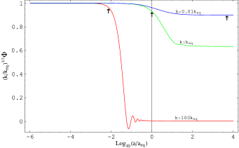
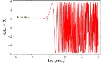
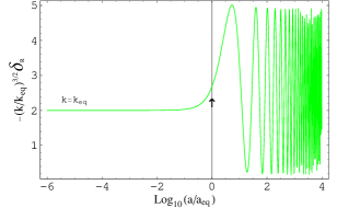
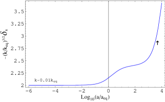
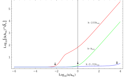
Given these initial conditions, it is fairly easy to integrate the equations forward in time and the numerical results are shown in Figs 2, 3, 4, 5. (In the figures is taken to be .) To understand the nature of the evolution, it is, however, useful to try out a few analytic approximations to Eqs. (72) – (74) which is what we will do now.
IV.1 Evolution for
Let us begin by considering very large wavelength modes corresponding to the limit. In this case adiabaticity is respected and we can set Then Eqs. (72), (73) become
| (77) |
Differentiating the first equation and using the second to eliminate , we get a second order equation for . Fortunately, this equation has an exact solution
| (78) |
[There is simple way of determining such an exact solution, which we will describe in Sec. IV.4.]. The initial condition on is chosen such that it goes to initially. The solution shows that, as long as the mode is bigger than the Hubble radius, the potential changes very little; it is constant initially as well as in the final matter dominated phase. At late times we see that so that decreases only by a factor (9/10) during the entire evolution if is a valid approximation.
IV.2 Evolution for in the radiation dominated phase
When the mode enters Hubble radius in the radiation dominated phase, we can no longer ignore the pressure terms. The pressure makes radiation density contrast oscillate and the gravitational potential, driven by this, also oscillates with a decay in the overall amplitude. An approximate procedure to describe this phase is to solve the coupled system, ignoring which is sub-dominant and then determine using the form of .
When is ignored, the problem reduces to the one solved earlier in Eqs (64), (65) with giving . Since can be expressed in terms of trigonometric functions, the solution given by Eq. (64) with , simplifies to
| (79) |
Note that as , we have . This solution shows that once the mode enters the Hubble radius, the potential decays in an oscillatory manner. For , the potential becomes . In the same limit, we get from Eq. (65) that
| (80) |
(This is analogous to Eq. (68) for the radiation dominated case.) This oscillation is seen clearly in Fig 3 and Fig.4 (left panel). The amplitude of oscillations is accurately captured by Eq. (80) for mode but not for ; this is to be expected since the mode is not entering in the radiation dominated phase.
Let us next consider matter perturbations during this phase. They grow, driven by the gravitational potential determined above. When , Eq.(73) becomes:
| (81) |
The is essentially determined by radiation and satisfies Eq. (61); using this, we can rewrite Eq. (81) as
| (82) |
The general solution to the homogeneous part of Eq. (82) (obtained by ignoring the right hand side) is ; hence the general solution to this equation is
| (83) |
For the growing mode varies as and dominates over the rest; hence we conclude that, matter, driven by , grows logarithmically during the radiation dominated phase for modes which are inside the Hubble radius.
IV.3 Evolution in the matter dominated phase
Finally let us consider the matter dominated phase, in which we can ignore the radiation and concentrate on Eq. (72) and Eq. (73). When these equations become:
| (84) |
These have a simple solution which we found earlier (see Eq. (69)):
| (85) |
In this limit, the matter perturbations grow linearly with expansion: . In fact this is the most dominant growth mode in the linear perturbation theory.
IV.4 An alternative description of matter-radiation system
Before proceeding further, we will describe an alternative procedure for discussing the perturbations in dark matter and radiation, which has some advantages. In the formalism we used above, we used perturbations in the energy density of radiation () and matter as the dependent variables. Instead, we now use perturbations in the total energy density, and the perturbations in the entropy per particle, as the new dependent variables. In terms of , these variables are defined as:
| (86) |
| (87) |
Given the equations for , one can obtain the corresponding equations for the new variables by straight forward algebra. It is convenient to express them as two coupled equations for and . After some direct but a bit tedious algebra, we get:
| (88) |
| (89) |
where we have defined
| (90) |
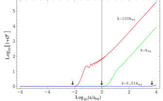
These equations show that the entropy perturbations and gravitational potential (which is directly related to total energy density perturbations) act as sources for each other. The coupling between the two arises through the right hand sides of Eq. (88) and Eq. (89). We also see that if we set as an initial condition, this is preserved to and — for long wave length modes — the evolves independent of . The solutions to the coupled equations obtained by numerical integration is shown in Fig.(2) right panel. The entropy perturbation till the mode enters Hubble radius and grows afterwards tracking either or whichever is the dominant energy density perturbation. To illustrate the behaviour of , let us consider the adiabatic perturbations at large scales with ; then the gravitational potential satisfies the equation:
| (91) |
which has the two independent solutions:
| (92) |
both of which diverge as . We need to combine these two solutions to find the general solution, keeping in mind that the general solution should be nonsingular and become a constant (say, unity) as . This fixes the linear combination uniquely:
| (93) |
Multiplying by we get the solution that was found earlier (see Eq. (78)). Given the form of and we can determine all other quantities. In particular, we get:
| (94) |
The corresponding velocity field, which we quote for future reference, is given by:
| (95) |
We conclude this section by mentioning another useful result related to Eq. (88). When , the equation for can be re-expressed as
| (96) |
where we have defined:
| (97) |
(The factor arises because of converting a gradient to the space; of course, when everything is done correctly, all physical quantities will be real.) Other equivalent alternative forms for , which are useful are:
| (98) |
For modes which are bigger than the Hubble radius, Eq. (96) shows that is conserved. When =constant, we can integrate Eq. (98) easily to obtain:
| (99) |
This is the easiest way to obtain the solution in Eq. (78).
The conservation law for also allows us to understand in a simple manner our previous result that only deceases by a factor when the mode remains bigger than Hubble radius as we evolve the equations from to . Let us compare the values of early in the radiation dominated phase and late in the matter dominated phase. From the first equation in Eq. (98), [using ] we find that, in the radiation dominated phase, ; late in the matter dominated phase, . Hence the conservation of gives which was the result obtained earlier. The expression in Eq. (99) also works at late times in the dominated or curvature dominated universe.
One key feature which should be noted in the study of linear perturbation theory is the different amount of growths for and . The either changes very little or decays; the grows in amplitude only by a factor of few. The physical reason, of course, is that the amplitude is frozen at super-Hubble scales and the pressure prevents the growth at sub-Hubble scales. In contrast, , which is pressureless, grows logarithmically in the radiation dominated era and linearly during the matter dominated era. Since the later phase lasts for a factor of in expansion, we get a fair amount of growth in .
V Transfer Function for matter perturbations
We now have all the ingredients to evolve the matter perturbation from an initial value at to the current epoch in the matter dominated phase at . Initially, the wavelength of the perturbation will be bigger than the Hubble radius and the perturbation will essentially remain frozen. When it enters the Hubble radius in the radiation dominated phase, it begins to grow but only logarithmically (see section IV.2 ) until the universe becomes matter dominated. In the final matter dominated phase, the perturbation grows linearly with expansion factor. The relation between final and initial perturbation can be obtained by combining these results.
Usually, one is more interested in the power spectrum and the power per logarithmic band in space . These quantities are defined in terms of through the equations:
| (100) |
It is therefore convenient to study the evolution of since its square will immediately give the power per logarithmic band in space.
Let us first consider a mode which enters the Hubble radius in the radiation dominated phase at the epoch . From the scaling relation, we find that . Hence
| (101) |
where two factors — as indicated — gives the growth in radiation (RD) and matter dominated (MD) phases. Let us next consider the modes that enter in the matter dominated phase. In this case, so that . Hence
| (102) |
To proceed further, we need to know the dependence of the perturbation when it enters the Hubble radius which, of course, is related to the mechanism that generates the initial power spectrum. The most natural choice will be that all the modes enter the Hubble radius with a constant amplitude at the time of entry. This would imply that the physical perturbations are scale invariant at the time of entering the Hubble radius, a possibility that was suggested by Zeldovich and Harrison zeldovich72 (years before inflation was invented!). We will see later that this is also true for perturbations generated by inflation and thus is a reasonable assumption at least in such models. Hence we shall assume
| (103) |
Using this we find that the current value of perturbation is given by
| (104) |
The corresponding power per logarithmic band is
| (105) |
The form for shows that the evolution imprints the scale on the power spectrum even though the initial power spectrum is scale invariant. For (for large spatial scales), the primordial form of the spectrum is preserved and the evolution only increases the amplitude preserving the shape. For (for small spatial scales), the shape is distorted and in general the power is suppressed in comparison with larger spatial scales. This arises because modes with small wavelengths enter the Hubble radius early on and have to wait till the universe becomes matter dominated in order to grow in amplitude. This is in contrast to modes with large wavelengths which continue to grow. It is this effect which suppresses the power at small wavelengths (for ) relative to power at larger wavelengths.
VI Temperature anisotropies of CMBR
We shall now apply the formalism we have developed to understand the temperature anisotropies in the cosmic microwave background radiation which is probably the most useful application of linear perturbation theory. We shall begin by developing the general formulation and the terminology which is used to describe the temperature anisotropies.
Towards every direction in the sky, we can define a fractional temperature fluctuation . Expanding this quantity in spherical harmonics on the sky plane as well as in terms of the spatial Fourier modes, we get the two relations:
| (106) |
where is the distance to the last scattering surface (LSS) from which we are receiving the radiation. The last equality allows us to define the expansion coefficients in terms of the temperature fluctuation in the Fourier space . Standard identities of mathematical physics now give
| (107) |
Next, let us consider the angular correlation function of temperature anisotropy, which is given by:
| (108) |
where the wedges denote an ensemble average. For a Gaussian random field of fluctuations we can express the ensemble average as . Using Eq. (107), we get a relation between and . Given , the ’s are given by:
| (109) |
Further, Eq. (108) now becomes:
| (110) |
Equation (110) shows that the mean-square value of temperature fluctuations and the quadrupole anisotropy corresponding to are given by
| (111) |
These can be explicitly computed if we know from the perturbation theory. (The motion of our local group through the CMBR leads to a large dipole contribution in the temperature anisotropy. In the analysis of CMBR anisotropies, this is usually subtracted out. Hence the leading term is the quadrupole with .)
It should be noted that, for a given , the is the average over all . For a Gaussian random field, one can also compute the variance around this mean value. It can be shown that this variance in is . In other words, there is an intrinsic root-mean-square fluctuation in the observed, mean value of ’s which is of the order of . It is not possible for any CMBR observations which measures the ’s to reduce its uncertainty below this intrinsic variance — usually called the “cosmic variance”. For large values of , the cosmic variance is usually sub-dominant to other observational errors but for low this is the dominant source of uncertainty in the measurement of ’s. Current WMAP observations are indeed only limited by cosmic variance at low-.
As an illustration of the formalism developed above, let us compute the ’s for low which will be contributed essentially by fluctuations at large spatial scales. Since these fluctuations will be dominated by gravitational effects, we can ignore the complications arising from baryonic physics and compute these using the formalism we have developed earlier.
We begin by noting that the redshift law of photons in the unperturbed Friedmann universe, , gets modified to the form in a perturbed FRW universe. The argument of the Planck spectrum will thus scale as
| (112) |
This is equivalent to a temperature fluctuation of the amount
| (113) |
at large scales. (Note that the observed is not just as one might have naively imagined.) To proceed further, we recall our large scale solution (see Eq. (78)) for the gravitational potential:
| (114) |
At we can take the asymptotic solution . Hence we get
| (115) |
We thus obtain the nice result that the observed temperature fluctuations at very large scales is simply related to the fluctuations of the gravitational potential at these scales. (For a discussion of the factor, see hwang ). Fourier transforming this result we get where is the conformal time at the last scattering surface. (This contribution is called Sachs-Wolfe effect.) It follows from Eq. (109) that the contribution to from the gravitational potential is
| (116) |
with
| (117) |
For a scale invariant spectrum, is a constant independent of . (Earlier on, in Eq. (103) we said that scale invariant spectrum has constant. These statements are equivalent since at the large scales because of Eq. (85) with the extra correction term in Eq. (85) being about for .) As we shall see later, inflation generates such a perturbation. In this case, it is conventional to introduce a constant amplitude and write:
| (118) |
Substituting this form into Eq. (116) and evaluating the integral, we find that
| (119) |
As an application of this result, let us consider the observations of COBE which measured the temperature fluctuations for the first time in 1992. This satellite obtained the RMS fluctuations and the quadrupole after smoothing over an angular scale of about . Hence the observed values are slightly different from those in Eq. (111). We have, instead,
| (120) |
Using Eqs. (118), (119) we find that
| (121) |
Given these two measurements, one can verify that the fluctuations are consistent with the scale invariant spectrum by checking their ratio. Further, the numerical value of the observed can be used to determine the amplitude . One finds that which sets the scale of fluctuations in the gravitational potential at the time when the perturbation enters the Hubble radius.
Incidentally, note that the solution corresponds to . At , taking , we get . Since we get . This shows that the amplitude of matter perturbations is a factor six larger that the amplitude of temperature anisotropy for our adiabatic initial conditions. In several other models, one gets . So, to reach a given level of nonlinearity in the matter distribution at later times, these models will require higher values of at decoupling. This is one reason for such models to be observationally ruled out.
There is another useful result which we can obtain from Eq. (109) along the same lines as we derived the Sachs-Wolfe effect. Whenever is a slowly varying function of , we can pull out this factor out of the integral and evaluate the integral over . This will give the result for any slowly varying
| (122) |
This is applicable even when different processes contribute to temperature anisotropies as long as they add in quadrature. While far from accurate, it allows one to estimate the effects rapidly.
VI.1 CMBR Temperature Anisotropy: More detailed theory
We shall now work out a more detailed theory of temperature anisotropies of CMBR so that one can understand the effects at small scales as well. A convenient starting point is the distribution function for photons with perturbed Planckian distribution, which we can write as:
| (123) |
The is the standard Planck spectrum for energy and we take to take care of the perturbations. In the absence of collisions, the distribution function is conserved along the trajectories of photons so that . So, in the presence of collisions, we can write the time evolution of the distribution function as
| (124) |
where the right hand side gives the contribution due to collisional terms. Equivalently, in terms of , the same equation takes the form:
| (125) |
To proceed further, we need the expressions for the two terms on the left hand side. First term, on using the standard expansion for total derivative, gives:
| (126) |
(Note that we are assuming so that the perturbations do not depend on the frequency of the photon.) To determine the second term, we note that it vanishes in the unperturbed Friedmann universe and arises essentially due to the variation of . Both the intrinsic time variation of as well as its variation along the photon path will contribute, giving:
| (127) |
(The minus sign arises from the fact that the we have in but in the spatial perturbations.) Putting all these together, we can bring the evolution equation Eq. (125) to the form:
| (128) |
Let us next consider the collision term, which can be expressed in the form:
| (129) | |||||
Each of the terms in the right hand side of the first line has a simple interpretation. The first term describes the removal of photons from the beam due to Thomson scattering with the electrons while the second term gives the scattering contribution into the beam. In a static universe, we expect these two terms to cancel if which fixes the relative coefficients of these two terms. The third term is a correction due to the fact that the electrons which are scattering the photons are not at rest relative to the cosmic frame. This leads to a Doppler shift which is accounted for by the third term. (We denote electron number density by rather than to avoid notational conflict with .)
Formally, Eq. (128) is a first order linear differential equation for . To eliminate the term which is linear in in the right hand side, we use the standard integrating factor where
| (130) |
We can then formally integrate Eq. (128) to get:
| (131) |
We can write
| (132) |
On integration, the first term gives zero at the lower limit and an unimportant constant (which does not depend on ). Using the rest of the terms, we can write Eq. (131) in the form:
| (133) | |||||
The first term gives the contribution due to the intrinsic time variation of the gravitational potential along the path of the photon and is called the integrated Sachs-Wolfe effect. In the second term one can make further simplifications. Note that is essentially unity (optically thin) for and zero (optically thick) for ; on the other hand, is zero for (all the free electrons have disappeared) and is large for . Hence the product is sharply peaked at (i.e. at with ). Treating this sharply peaked quantity as essentially a Dirac delta function (usually called the instantaneous recombination approximation) we can approximate the second term in Eq. (133) as a contribution occurring just on the LSS:
| (134) |
In the second term we have put for and for .
Once we know and on the LSS from perturbation theory, we can take a Fourier transform of this result to obtain and use Eq. (109) to compute . At very large scales the velocity term is sub-dominant and we get back the Sachs-Wolfe effect derived earlier in Eq. (118). For understanding the small scale effects, we need to introduce baryons into the picture which is our next task.
VI.2 Description of photon-baryon fluid
To study the interaction of photons and baryons in the fluid limit, we need to again start from the continuity equation and Euler equation. In Fourier space, the continuity equation is same as the one we had before (see Eq. (52)):
| (135) |
The Euler equations, however, gets modified; for photons, it becomes:
| (136) |
The first two terms in the right hand side are exactly the same as the ones in Eq. (55). The last term is analogous to a viscous drag force between the photons and baryons which arises because of the non zero relative velocity between the two fluids. The coupling is essentially due to Thomson scattering which leads to the factor . (The notation, and the physics, is the same as in Eq. (130)). The corresponding Euler equation for the baryons is:
| (137) |
where
| (138) |
Again, the first two terms in the right hand side of Eq. (137) are the same as what we had before in Eq. (55). The last term has the same interpretation as in the case of Euler equation Eq. (136) for photons, except for the factor . This quantity essentially takes care of the inertia of baryons relative to photons. Note that the the conserved momentum density of photon-baryon fluid has the form
| (139) |
which accounts for the extra factor in Eq. (137).
We can now combine the Eqs. (135), (136), (137) to obtain, to lowest order in the equation:
| (140) |
with
| (141) |
An exact solution to this equation is difficult to obtain. However, we can try to understand several features by an approximate method in which we treat the time variation of to be small. In that case, we can drop the terms on both sides of the equation. Since we know that the physically relevant temperature fluctuation is , we can recast the above equation for as:
| (142) |
Let us further ignore the time variation of all terms (especially on the right hand side). Then, the solution is just . To fix the initial conditions which determine and , we recall that early on , we have (see Eq. (115)) and corresponding velocity should vanish. This gives the solution:
| (143) |
(One can do a little better by using WKB approximation in which can be replaced by the integral of over but it is not very important.) Given this solution, one can proceed as before and compute the ’s. Adding the effects of [] and that of [] in quadrature and noticing that the angular average of we can estimate the for scale invariant ( ) spectrum to be:
| (144) |
with with . The key feature is, of course, the maxima and minima which arises from the trigonometric functions. The peaks of are determined by the condition ; that is
| (145) |
More precise work gives the first peak at It is also clear that because of non zero the peaks are larger when the cosine term is negative; that is, the odd peaks corresponding to have larger amplitudes than the even peaks with .
Incidentally, the above approximation is not very good for modes which enter the Hubble radius during the radiation dominated phase since does evolve with time (and decays) in the radiation dominated phase. We saw that asymptotically in this phase (see Eq. (80)). From Eq. (80) we find that during this phase, for modes which are inside the Hubble radius, we can take , so that . On the other hand, at very large scale, the amplitude was . Hence the amplitude of the modes that enter the horizon during the radiation dominated phase is enhanced by a factor , relative to the large scale amplitude contributed by modes which enter during matter dominated phase. This is essentially due to the driving term which is nonzero in the radiation dominated phase but zero in the matter dominated phase. (In reality, the enhancement is smaller because the relevant modes have rather than ; see Figs. 3 and 4.)
If this were the whole story, we will see a series of peaks and troughs in the temperature anisotropies as a function of angular scale. In reality, however, there are processes which damp out the anisotropies at small angular scales (large -) so that only the first few peaks and troughs are really relevant. We will now discuss two key damping mechanisms which are responsible for this.
The first one is the finite width of the last scattering surface which makes it uncertain from which event we are receiving the photons. In general, if is the probability that the photon was last scattered at redshift , then we can write:
| (146) |
From Eq. (41) we know that is a Gaussian with width . This corresponds to a length scale
| (147) |
over which the temperature fluctuations will be smoothed out.
It turns out that there is another effect, which is slightly more important. This arises from the fact that the photon-baryon fluid is not tightly coupled and the photons can diffuse through the fluid. This diffusion can be modeled as a random walk and the root mean square distance traveled by the photon during this diffusion process will smear the temperature anisotropies over that length scale. This photon diffusion length scale can be estimated as follows:
| (148) |
Integrating, we find the mean square distance traveled by the photon to be
| (149) |
The corresponding proper length scale below which photon diffusion will wipe out temperature anisotropies is:
| (150) |
It turns out that this is the dominant sources of damping of temperature anisotropies at large .
VII Generation of initial perturbations from inflation
In the description of linear perturbation theory given above, we assumed that some small perturbations existed in the early universe which are amplified through gravitational instability. To provide a complete picture we need a mechanism for generation of these initial perturbations. One such mechanism is provided by inflationary scenario which allows for the quantum fluctuations in the field driving the inflation to provide classical energy density perturbations at a late epoch. (Originally inflationary scenarios were suggested as pseudo-solutions to certain pseudo-problems; that is only of historical interest today and the only reason to take the possibility of an inflationary phase in the early universe seriously is because it provides a mechanism for generating these perturbations.) We shall now discuss how this can come about.
The basic assumption in inflationary scenario is that the universe underwent a rapid — nearly exponential — expansion for a brief period of time in very early universe. The simplest way of realizing such a phase is to postulate the existence of a scalar field with a nearly flat potential. The dynamics of the universe, driven by a scalar field source, is described by:
| (151) |
where . If the potential is nearly flat for certain range of , we can introduce the “ slow roll-over” approximation, under which these equations become:
| (152) |
For this slow roll-over to last for reasonable length of time, we need to assume that the terms ignored in the Eq. (151) are indeed small. This can be quantified in terms of the parameters:
| (153) |
which are taken to be small. Typically the inflation ends when this assumption breaks down. If such an inflationary phase lasts up to some time then the universe would have undergone an expansion by a factor during the interval where
| (154) |
One usually takes or so.
Before proceeding further, we would like to make couple of comments regarding such an inflationary phase. To begin with, it is not difficult to obtain exact solutions for with rapid expansion by tailoring the potential for the scalar field. In fact, given any and thus a , one can determine a potential for a scalar field such that Eq. (151) are satisfied (see the first reference in tptachyon ). One can verify that, this is done by the choice:
| (155) |
Given any , these equations give and thus implicitly determine the necessary . As an example, note that a power law inflation, (with ) is generated by:
| (156) |
while an exponential of power law
| (157) |
can arise from
| (158) |
Thus generating a rapid expansion in the early universe is trivial if we are willing to postulate scalar fields with tailor made potentials. This is often done in the literature.
The second point to note regarding any inflationary scenarios is that the modes with reasonable size today originated from sub-Planck length scales early on. A scale today will be
| (159) |
at the end of inflation (if inflation took place at GUT scales) and
| (160) |
at the beginning of inflation if the inflation changed the scale factor by . Note that for Mpc!! Most structures in the universe today correspond to transplanckian scales at the start of the inflation. It is not clear whether we can trust standard physics at early stages of inflation or whether transplanckian effects will lead to observable effects transplanck ; dispersion .
Let us get back to conventional wisdom and consider the evolution of perturbations in a universe which underwent exponential inflation. During the inflationary phase the grows exponentially and hence the wavelength of any perturbation will also grow with it. The Hubble radius, on the other hand, will remain constant. It follows that, one can have situation in which a given mode has wavelength smaller than the Hubble radius at the beginning of the inflation but grows and becomes bigger than the Hubble radius as inflation proceeds. It is conventional to say that a perturbation of comoving wavelength “leaves the Hubble radius” when at some time . For the wavelength of the perturbation is bigger than the Hubble radius. Eventually the inflation ends and the universe becomes radiation dominated. Then the wavelength will grow ( slower than the Hubble radius () and will enter the Hubble radius again during . Our first task is to relate the amplitude of the perturbation at with the perturbation at .
We know that for modes bigger than Hubble radius, we have the conserved quantity (see Eq. (97)
| (161) |
At the time of re-entry, the universe is radiation dominated and . On the other hand, during inflation, we can write the scalar field as a dominant homogeneous part plus a small, spatially varying fluctuation: . Perturbing the equation in Eq. (151) for the scalar field, we find that the homogeneous mode satisfies Eq. (151) while the perturbation, in Fourier space satisfies:
| (162) |
Further, the energy momentum tensor for the scalar field gives [with the “dot” denoting ]:
| (163) |
It is easy to see that is negligible at since
| (164) |
Therefore,
| (165) |
Using the conservation law we get
| (166) |
Thus, given a perturbation of the scalar field during inflation, we can compute its value at the time of re-entry, which — in turn — can be used to compare with observations.
Equation (166) connects a classical energy density perturbation at the time of exit with the corresponding quantity at the time of re-entry. The next important — and conceptually difficult — question is how we can obtain a c-number field from a quantum scalar field. There is no simple answer to this question and one possible way of doing it is as follows: Let us start with the quantum operator for a scalar field decomposed into the Fourier modes with denoting an infinite set of operators:
| (167) |
We choose a quantum state such the expectation value of vanishes for all non-zero so that the expectation value of gives the homogeneous mode that drives the inflation. The quantum fluctuation around this homogeneous part in a quantum state is given by
| (168) |
It is easy to verify that this fluctuation is just the Fourier transform of the two-point function in this state:
| (169) |
Since characterises the quantum fluctuations, it seems reasonable to introduce a c-number field by the definition:
| (170) |
This c-number field will have same c-number power spectrum as the quantum fluctuations. Hence we may take this as our definition of an equivalent classical perturbation. (There are more sophisticated ways of getting this result but none of them are fundamentally more sound that the elementary definition given above. There is a large literature on the subject of quantum to classical transition, especially in the context of gravity; see e.g.semicgrav ) We now have all the ingredients in place. Given the quantum state , one can explicitly compute and then — using Eq. (166) with — obtain the density perturbations at the time of re-entry.
The next question we need to address is what is . The free quantum field theory in the Friedmann background is identical to the quantum mechanics of a bunch of time dependent harmonic oscillators, each labelled by a wave vector . The action for a free scalar field in the Friedmann background
| (171) |
can be thought of as the sum over the actions for an infinite set of harmonic oscillators with mass and frequency . (To be precise, one needs to treat the real and imaginary parts of the Fourier transform as independent oscillators and restrict the range of ; just pretending that is real amounts the same thing.) The quantum state of the field is just an infinite product of the quantum state for each of the harmonic oscillators and satisfies the Schrodinger equation
| (172) |
If the quantum state of any given oscillator, labelled by , is given at some initial time, , we can evolve it to final time:
| (173) |
where is known in terms of the solutions to the classical equations of motion and is the initial state. There is nothing non-trivial in the mathematics, but the physics is completely unknown. The real problem is that unfortunately — in spite of confident assertions in the literature occasionally — we have no clue what is. So we need to make more assumptions to proceed further.
One natural choice is the following: It turns out that, Gaussian states of the form
| (174) |
preserve their form under evolution governed by the Schrodinger equation in Eq. (172). Substituting Eq. (174) in Eq. (172) we can determine the ordinary differential equation which governs . (The is trivially fixed by normalization.) Simple algebra shows that can be expressed in the form
| (175) |
where is the solution to the classical equation of motion:
| (176) |
For the quantum state in Eq. (174), the fluctuations are characterized by
| (177) |
Since one can take different choices for the solutions of Eq. (176) one get different values for and different spectra for perturbations. Any prediction one makes depends on the choice of mode functions. One possibility is to choose the modes so that represents the instantaneous vacuum state of the oscillators at some time . (That is Re say). The final result will then depend on the choice for . One can further make an assumption that we are interested in the limit of ; that is the quantum state is an instantaneous ground state in the infinite past. It is easy to show that this corresponds to choosing the following solution to Eq. (176):
| (178) |
which is usually called the Bunch-Davies vacuum. For this choice,
| (179) |
where the second result is at which is what we need to use in Eq. (166), (Numerical factors of order unity cannot be trusted in this computation). We can now determine the amplitude of the perturbation when it re-enters the Hubble radius. Eq. (166) gives:
| (180) |
One sees that the result is scale invariant in the sense that is independent of .
It is sometimes claimed in the literature that scale invariant spectrum is a prediction of inflation. This is simply wrong. One has to make several other assumptions including an all important choice for the quantum state (about which we know nothing) to obtain scale invariant spectrum. In fact, one can prove that, given any power spectrum , one can find a quantum state such that this power spectrum is generated (for an explicit construction, see the last reference in transplanck ). So whatever results are obtained by observations can be reconciled with inflationary generation of perturbations.
To conclude the discussion, let us work out the perturbations for one specific case. Let us consider the case of the model for which
| (181) |
Using
| (182) |
we can write
| (183) |
so that the result in Eq. (180) becomes:
| (184) |
We do get scale invariant spectrum but the amplitude has a serious problem. If we take and note that observations require we need to take for getting consistent values. Such a fine tuning of a dimensionless coupling constant is fairly ridiculous; but over years inflationists have learnt to successfully forget this embarrassment.
Our formalism can also be used to estimate the deviation of the power spectrum from the scale invariant form. To the lowest order we have
| (185) |
Let us define the deviation from the scale invariant index by . Using
| (186) |
one finds that
| (187) |
Thus, as long as and are small we do have ; what is more, given a potential one can estimate and and thus the deviation .
Finally, note that the same process can also generate spin-2 perturbations. If we take the normalised gravity wave amplitude as , the mode function behaves like a scalar field. (The normalisation is dictated by the fact that the action for the perturbation should reduce to that of a spin-2 field.) The corresponding power spectrum of gravity waves is
| (188) |
Comparing the two results
| (189) |
we get . Further, if (see Eq. (187) with ) we have the relation which connects three quantities, all of which are independently observable in principle. If these are actually measured in future it could act as a consistency check of the inflationary paradigm.
VIII The Dark Energy
It is rather frustrating that the only component of the universe which we understand theoretically is the radiation! While understanding the baryonic and dark matter components [in particular the values of and ] is by no means trivial, the issue of dark energy is lot more perplexing, thereby justifying the attention it has received recently. In this section we will discuss several aspects of the dark energy problem.
The key observational feature of dark energy is that — treated as a fluid with a stress tensor dia — it has an equation state with at the present epoch. The spatial part of the geodesic acceleration (which measures the relative acceleration of two geodesics in the spacetime) satisfies an exact equation in general relativity given by:
| (190) |
This shows that the source of geodesic acceleration is and not . As long as , gravity remains attractive while can lead to repulsive gravitational effects. In other words, dark energy with sufficiently negative pressure will accelerate the expansion of the universe, once it starts dominating over the normal matter. This is precisely what is established from the study of high redshift supernova, which can be used to determine the expansion rate of the universe in the past sn .
The simplest model for a fluid with negative pressure is the cosmological constant (for some recent reviews, see cc ) with constant. If the dark energy is indeed a cosmological constant, then it introduces a fundamental length scale in the theory , related to the constant dark energy density by . In classical general relativity, based on the constants and , it is not possible to construct any dimensionless combination from these constants. But when one introduces the Planck constant, , it is possible to form the dimensionless combination . Observations then require . As has been mentioned several times in literature, this will require enormous fine tuning. What is more, in the past, the energy density of normal matter and radiation would have been higher while the energy density contributed by the cosmological constant does not change. Hence we need to adjust the energy densities of normal matter and cosmological constant in the early epoch very carefully so that around the current epoch. This raises the second of the two cosmological constant problems: Why is it that at the current phase of the universe ?
Because of these conceptual problems associated with the cosmological constant, people have explored a large variety of alternative possibilities. The most popular among them uses a scalar field with a suitably chosen potential so as to make the vacuum energy vary with time. The hope then is that, one can find a model in which the current value can be explained naturally without any fine tuning. A simple form of the source with variable are scalar fields with Lagrangians of different forms, of which we will discuss two possibilities:
| (191) |
Both these Lagrangians involve one arbitrary function . The first one, , which is a natural generalization of the Lagrangian for a non-relativistic particle, , is usually called quintessence (for a small sample of models, see phiindustry ; there is an extensive and growing literature on scalar field models and more references can be found in the reviews in ref.cc ). When it acts as a source in Friedmann universe, it is characterized by a time dependent with
| (192) |
The structure of the second Lagrangian (which arise in string theory asen ) in Eq. (191) can be understood by a simple analogy from special relativity. A relativistic particle with (one dimensional) position and mass is described by the Lagrangian . It has the energy and momentum which are related by . As is well known, this allows the possibility of having massless particles with finite energy for which . This is achieved by taking the limit of and , while keeping the ratio in finite. The momentum acquires a life of its own, unconnected with the velocity , and the energy is expressed in terms of the momentum (rather than in terms of ) in the Hamiltonian formulation. We can now construct a field theory by upgrading to a field . Relativistic invariance now requires to depend on both space and time [] and to be replaced by . It is also possible now to treat the mass parameter as a function of , say, thereby obtaining a field theoretic Lagrangian . The Hamiltonian structure of this theory is algebraically very similar to the special relativistic example we started with. In particular, the theory allows solutions in which , simultaneously, keeping the energy (density) finite. Such solutions will have finite momentum density (analogous to a massless particle with finite momentum ) and energy density. Since the solutions can now depend on both space and time (unlike the special relativistic example in which depended only on time), the momentum density can be an arbitrary function of the spatial coordinate. The structure of this Lagrangian is similar to those analyzed in a wide class of models called K-essence kessence and provides a rich gamut of possibilities in the context of cosmology tptachyon ; tachyon .
Since the quintessence field (or the tachyonic field) has an undetermined free function , it is possible to choose this function in order to produce a given . To see this explicitly, let us assume that the universe has two forms of energy density with where arises from any known forms of source (matter, radiation, …) and is due to a scalar field. Let us first consider quintessence. Here, the potential is given implicitly by the form ellis ; tptachyon .
| (193) |
where and prime denotes differentiation with respect to . (The result used in Eq. (155) is just a special case of this when ) Given any , these equations determine and and thus the potential . Every quintessence model studied in the literature can be obtained from these equations.
Similar results exists for the tachyonic scalar field as well tptachyon . For example, given any , one can construct a tachyonic potential so that the scalar field is the source for the cosmology. The equations determining are now given by:
| (194) |
Equations (194) completely solve the problem. Given any , these equations determine and and thus the potential . A wide variety of phenomenological models with time dependent cosmological constant have been considered in the literature all of which can be mapped to a scalar field model with a suitable .
While the scalar field models enjoy considerable popularity (one reason being they are easy to construct!) it is very doubtful whether they have helped us to understand the nature of the dark energy at any deeper level. These models, viewed objectively, suffer from several shortcomings:
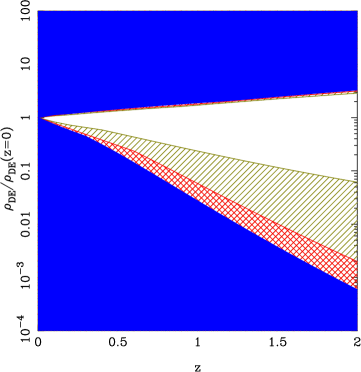
-
•
They completely lack predictive power. As explicitly demonstrated above, virtually every form of can be modeled by a suitable “designer” .
-
•
These models are degenerate in another sense. The previous discussion illustrates that even when is known/specified, it is not possible to proceed further and determine the nature of the scalar field Lagrangian. The explicit examples given above show that there are at least two different forms of scalar field Lagrangians (corresponding to the quintessence or the tachyonic field) which could lead to the same . (See the second paper in ref.tptirthsn1 for an explicit example of such a construction.)
-
•
All the scalar field potentials require fine tuning of the parameters in order to be viable. This is obvious in the quintessence models in which adding a constant to the potential is the same as invoking a cosmological constant. So to make the quintessence models work, we first need to assume the cosmological constant is zero. These models, therefore, merely push the cosmological constant problem to another level, making it somebody else’s problem!.
-
•
By and large, the potentials used in the literature have no natural field theoretical justification. All of them are non-renormalisable in the conventional sense and have to be interpreted as a low energy effective potential in an ad hoc manner.
-
•
One key difference between cosmological constant and scalar field models is that the latter lead to a which varies with time. If observations have demanded this, or even if observations have ruled out at the present epoch, then one would have been forced to take alternative models seriously. However, all available observations are consistent with cosmological constant () and — in fact — the possible variation of is strongly constrained jbp as shown in Figure 6.
-
•
While on the topic of observational constraints on , it must be stressed that: (a) There is fair amount of tension between WMAP and SN data and one should be very careful about the priors used in these analysis. (b) There is no observational evidence for . (c) It is likely that more homogeneous, future, data sets of SN might show better agreement with WMAP results. (For more details related to these issues, see the last reference in jbp .)
The observational and theoretical features described above suggests that one should consider cosmological constant as the most natural candidate for dark energy. Though it leads to well know fine tuning problems, it also has certain attractive features that need to kept in mind.
-
•
Cosmological constant is the most economical [just one number] and simplest explanation for all the observations. We stress that there is absolutely no evidence for variation of dark energy density with redshift, which is consistent with the assumption of cosmological constant .
-
•
Once we invoke the cosmological constant classical gravity will be described by the three constants and . It is not possible to obtain a dimensionless quantity from these; so, within classical theory, there is no fine tuning issue. Since , it is obvious that the cosmological constant is telling us something regarding quantum gravity, indicated by the combination . An acid test for any quantum gravity model will be its ability to explain this value; needless to say, all the currently available models — strings, loops etc. — flunk this test.
-
•
So, if dark energy is indeed cosmological constant this will be the greatest contribution from cosmology to fundamental physics. It will be unfortunate if we miss this chance by invoking some scalar field epicycles!
In this context, it is worth stressing another peculiar feature of cosmological constant when it is treated as a clue to quantum gravity. It is well known that, based on energy scales, the cosmological constant problem is an infra red problem par excellence. At the same time, it is a relic of a quantum gravitational effect or principle of unknown nature. An analogy choices will be helpful to illustrate this point. Suppose one solves the Schrodinger equation for the Helium atom for the quantum states of the two electrons . When the result is compared with observations, one will find that only half the states — those in which is antisymmetric under interchange — are realized in nature. But the low energy Hamiltonian for electrons in the Helium atom has no information about this effect! Here is low energy (IR) effect which is a relic of relativistic quantum field theory (spin-statistics theorem) that is totally non perturbative, in the sense that writing corrections to the Helium atom Hamiltonian in some expansion will not reproduce this result. The current value of cosmological constant could very well be related to quantum gravity in a similar way. There must exist a deep principle in quantum gravity which leaves its non perturbative trace even in the low energy limit that appears as the cosmological constant .
Let us now turn our attention to few of the many attempts to understand the cosmological constant. The choice is, of course, dictated by personal bias and is definitely a non-representative sample. A host of other approaches exist in literature, some of which can be found in catchall .
VIII.1 Gravitational Holography
One possible way of addressing this issue is to simply eliminate from the gravitational theory those modes which couple to cosmological constant. If, for example, we have a theory in which the source of gravity is rather than in Eq. (190), then cosmological constant will not couple to gravity at all. (The non linear coupling of matter with gravity has several subtleties; see eg. gravitonmyth .) Unfortunately it is not possible to develop a covariant theory of gravity using as the source. But we can probably gain some insight from the following considerations. Any metric can be expressed in the form such that so that . From the action functional for gravity
| (195) |
it is obvious that the cosmological constant couples only to the conformal factor . So if we consider a theory of gravity in which is kept constant and only is varied, then such a model will be oblivious of direct coupling to cosmological constant. If the action (without the term) is varied, keeping , say, then one is lead to a unimodular theory of gravity that has the equations of motion with zero trace on both sides. Using the Bianchi identity, it is now easy to show that this is equivalent to the usual theory with an arbitrary cosmological constant. That is, cosmological constant arises as an undetermined integration constant in this model unimod .
The same result arises in another, completely different approach to gravity. In the standard approach to gravity one uses the Einstein-Hilbert Lagrangian which has a formal structure . If the surface term obtained by integrating is ignored (or, more formally, canceled by an extrinsic curvature term) then the Einstein’s equations arise from the variation of the bulk term which is the non-covariant Lagrangian. There is, however, a remarkable relation between and :
| (196) |
which allows a dual description of gravity using either or ! It is possible to obtain the dynamics of gravity tpholo from an approach which uses only the surface term of the Hilbert action; we do not need the bulk term at all!. This suggests that the true degrees of freedom of gravity for a volume reside in its boundary — a point of view that is strongly supported by the study of horizon entropy, which shows that the degrees of freedom hidden by a horizon scales as the area and not as the volume. The resulting equations can be cast in a thermodynamic form and the continuum spacetime is like an elastic solid (see e.g. sakharov ) with Einstein’s equations providing the macroscopic description. Interestingly, the cosmological constant arises again in this approach as a undetermined integration constant but closely related to the ‘bulk expansion’ of the solid.
While this is all very interesting, we still need an extra physical principle to fix the value (even the sign) of cosmological constant. One possible way of doing this is to interpret the term in the action as a Lagrange multiplier for the proper volume of the spacetime. Then it is reasonable to choose the cosmological constant such that the total proper volume of the universe is equal to a specified number. While this will lead to a cosmological constant which has the correct order of magnitude, it has several obvious problems. First, the proper four volume of the universe is infinite unless we make the spatial sections compact and restrict the range of time integration. Second, this will lead to a dark energy density which varies as (corresponding to ) which is ruled out by observations.
VIII.2 Cosmic Lenz law
Another possibility which has been attempted in the literature tries to “cancel out” the cosmological constant by some process, usually quantum mechanical in origin. One of the simplest ideas will be to ask whether switching on a cosmological constant will lead to a vacuum polarization with an effective energy momentum tensor that will tend to cancel out the cosmological constant. A less subtle way of doing this is to invoke another scalar field (here we go again!) such that it can couple to cosmological constant and reduce its effective value lenz . Unfortunately, none of this could be made to work properly. By and large, these approaches lead to an energy density which is either (where is the Planck length) or to (where is the Hubble radius associated with the cosmological constant ). The first one is too large while the second one is too small!
VIII.3 Geometrical Duality in our Universe
While the above ideas do not work, it gives us a clue. A universe with two length scales and will be asymptotically De Sitter with at late times. There are some curious features in such a universe which we will now describe. Given the two length scales and , one can construct two energy scales and in natural units (). There is sufficient amount of justification from different theoretical perspectives to treat as the zero point length of spacetime zeropoint , giving a natural interpretation to . The second one, also has a natural interpretation. The universe which is asymptotically De Sitter has a horizon and associated thermodynamics ghds with a temperature and the corresponding thermal energy density . Thus determines the highest possible energy density in the universe while determines the lowest possible energy density in this universe. As the energy density of normal matter drops below this value, the thermal ambience of the De Sitter phase will remain constant and provide the irreducible ‘vacuum noise’. Note that the dark energy density is the the geometric mean between the two energy densities. If we define a dark energy length scale such that then is the geometric mean of the two length scales in the universe. (Incidentally, mm is macroscopic; it is also pretty close to the length scale associated with a neutrino mass of eV; another intriguing coincidence ?!)
Using the characteristic length scale of expansion, the Hubble radius , we can distinguish between three different phases of such a universe. The first phase is when the universe went through a inflationary expansion with constant; the second phase is the radiation/matter dominated phase in which most of the standard cosmology operates and increases monotonically; the third phase is that of re-inflation (or accelerated expansion) governed by the cosmological constant in which is again a constant. The first and last phases are time translation invariant; that is, constant is an (approximate) invariance for the universe in these two phases. The universe satisfies the perfect cosmological principle and is in steady state during these phases!
In fact, one can easily imagine a scenario in which the two De Sitter phases (first and last) are of arbitrarily long duration plumian . If the final De Sitter phase does last forever; as regards the inflationary phase, nothing prevents it from lasting for arbitrarily long duration. Viewed from this perspective, the in between phase — in which most of the ‘interesting’ cosmological phenomena occur — is of negligible measure in the span of time. It merely connects two steady state phases of the universe.
While the two De Sitter phases can last forever in principle, there is a natural cut off length scale in both of them which makes the region of physical relevance to be finite plumian . Let us first discuss the case of re-inflation in the late universe. As the universe grows exponentially in the phase 3, the wavelength of CMBR photons are being redshifted rapidly. When the temperature of the CMBR radiation drops below the De Sitter temperature (which happens when the wavelength of the typical CMBR photon is stretched to the .) the universe will be essentially dominated by the vacuum thermal noise ghds due to the horizon in the De Sitter phase. This happens when the expansion factor is determined by the equation . Let be the epoch at which cosmological constant started dominating over matter, so that . Then we find that the dynamic range of the phase 3 is
| (197) |
Interestingly enough, one can also impose a similar bound on the physically relevant duration of inflation. We know that the quantum fluctuations, generated during this inflationary phase, could act as seeds of structure formation in the universe. Consider a perturbation at some given wavelength scale which is stretched with the expansion of the universe as . During the inflationary phase, the Hubble radius remains constant while the wavelength increases, so that the perturbation will ‘exit’ the Hubble radius at some time. In the radiation dominated phase, the Hubble radius grows faster than the wavelength . Hence, normally, the perturbation will ‘re-enter’ the Hubble radius at some time. If there was no re-inflation, all wavelengths will re-enter the Hubble radius sooner or later. But if the universe undergoes re-inflation, then the Hubble radius ‘flattens out’ at late times and some of the perturbations will never reenter the Hubble radius ! If we use the criterion that we need the perturbation to reenter the Hubble radius, we get a natural bound on the duration of inflation which is of direct astrophysical relevance. Consider a perturbation which leaves the Hubble radius () during the inflationary epoch at . It will grow to the size at a later epoch. We want to determine such that this length scale grows to just when the dark energy starts dominating over matter; that is at the epoch . This gives so that . On the other hand, the inflation ends at where where is the temperature to which the universe has been reheated at the end of inflation. Using these two results we can determine the dynamic range of this phase 1 to be
| (198) |
where we have used the fact that, for a GUTs scale inflation with we have . If we consider a quantum gravitational, Planck scale, inflation with , the ranges in Eq. (197) and Eq. (198) are approximately equal.
This fact is definitely telling us something regarding the duality between Planck scale and Hubble scale or between the infrared and ultraviolet limits of the theory. The mystery is compounded by the fact the asymptotic De Sitter phase has an observer dependent horizon and related thermal properties ghds . Recently, it has been shown — in a series of papers, see ref.tpholo — that it is possible to obtain classical relativity from purely thermodynamic considerations. It is difficult to imagine that these features are unconnected and accidental; at the same time, it is difficult to prove a definite connection between these ideas and the cosmological constant.
VIII.4 Gravity as detector of the vacuum energy
Finally, we will describe an idea which does lead to the correct value of cosmological constant. The conventional discussion of the relation between cosmological constant and vacuum energy density is based on evaluating the zero point energy of quantum fields with an ultraviolet cutoff and using the result as a source of gravity. Any reasonable cutoff will lead to a vacuum energy density which is unacceptably high. This argument, however, is too simplistic since the zero point energy — obtained by summing over the — has no observable consequence in any other phenomena and can be subtracted out by redefining the Hamiltonian. The observed non trivial features of the vacuum state of QED, for example, arise from the fluctuations (or modifications) of this vacuum energy rather than the vacuum energy itself. This was, in fact, known fairly early in the history of cosmological constant problem and is stressed by Zeldovich zeldo who explicitly calculated one possible contribution to fluctuations after subtracting away the mean value. This suggests that we should consider the fluctuations in the vacuum energy density in addressing the cosmological constant problem.
If the vacuum probed by the gravity can readjust to take away the bulk energy density , quantum fluctuations can generate the observed value . One of the simplest models tpcqglamda which achieves this uses the fact that, in the semi-classical limit, the wave function describing the universe of proper four-volume will vary as . If we treat as conjugate variables then uncertainty principle suggests . If the four volume is built out of Planck scale substructures, giving , then the Poisson fluctuations will lead to giving . (This idea can be a more quantitative; see tpcqglamda ).
Similar viewpoint arises, more rigorously, when we study the question of detecting the energy density using gravitational field as a probe. Recall that an Unruh-DeWitt detector with a local coupling to the field actually responds to rather than to the field itself probe . Similarly, one can use the gravitational field as a natural “detector” of energy momentum tensor with the standard coupling . Such a model was analysed in detail in ref. tptptmunu and it was shown that the gravitational field responds to the two point function . In fact, it is essentially this fluctuations in the energy density which is computed in the inflationary models (see Eq. (170)) as the seed source for gravitational field, as stressed in ref. tplp . All these suggest treating the energy fluctuations as the physical quantity “detected” by gravity, when one needs to incorporate quantum effects. If the cosmological constant arises due to the energy density of the vacuum, then one needs to understand the structure of the quantum vacuum at cosmological scales. Quantum theory, especially the paradigm of renormalization group has taught us that the energy density — and even the concept of the vacuum state — depends on the scale at which it is probed. The vacuum state which we use to study the lattice vibrations in a solid, say, is not the same as vacuum state of the QED.
In fact, it seems inevitable that in a universe with two length scale , the vacuum fluctuations will contribute an energy density of the correct order of magnitude . The hierarchy of energy scales in such a universe, as detected by the gravitational field has plumian ; tpvacfluc the pattern
| (199) |
The first term is the bulk energy density which needs to be renormalized away (by a process which we do not understand at present); the third term is just the thermal energy density of the De Sitter vacuum state; what is interesting is that quantum fluctuations in the matter fields inevitably generate the second term.
The key new ingredient arises from the fact that the properties of the vacuum state depends on the scale at which it is probed and it is not appropriate to ask questions without specifying this scale. If the spacetime has a cosmological horizon which blocks information, the natural scale is provided by the size of the horizon, , and we should use observables defined within the accessible region. The operator , corresponding to the total energy inside a region bounded by a cosmological horizon, will exhibit fluctuations since vacuum state is not an eigenstate of this operator. The corresponding fluctuations in the energy density, will now depend on both the ultraviolet cutoff as well as . To obtain which scales as we need to have ; that is, the square of the energy fluctuations should scale as the surface area of the bounding surface which is provided by the cosmic horizon. Remarkably enough, a rigorous calculation tpvacfluc of the dispersion in the energy shows that for , the final result indeed has the scaling
| (200) |
where the constant depends on the manner in which ultra violet cutoff is imposed. Similar calculations have been done (with a completely different motivation, in the context of entanglement entropy) by several people and it is known that the area scaling found in Eq. (200), proportional to , is a generic feature area . For a simple exponential UV-cutoff, but cannot be computed reliably without knowing the full theory. We thus find that the fluctuations in the energy density of the vacuum in a sphere of radius is given by
| (201) |
The numerical coefficient will depend on as well as the precise nature of infrared cutoff radius (like whether it is or etc.). It would be pretentious to cook up the factors to obtain the observed value for dark energy density. But it is a fact of life that a fluctuation of magnitude will exist in the energy density inside a sphere of radius if Planck length is the UV cut off. One cannot get away from it. On the other hand, observations suggest that there is a of similar magnitude in the universe. It seems natural to identify the two, after subtracting out the mean value by hand. Our approach explains why there is a surviving cosmological constant which satisfies which — in our opinion — is the problem.
Acknowledgement
I thank J. Alcaniz for his friendship and warm hospitality during the X Special Courses at Observatorio Nacional, Rio de Janeiro, Brazil and for persuading me to write up my lecture notes. I am grateful to Gaurang Mahajan for help in generating the figures.
References
- (1) P. de Bernardis et al., Nature 404, 955 (2000); A. Balbi et al., Ap.J. 545, L1 (2000); S. Hanany et al., Ap.J. 545, L5 (2000); T.J. Pearson et al., Ap.J. 591, 556 (2003); C.L. Bennett et al, Ap. J. Suppl. 148, 1 (2003); D. N. Spergel et al., Ap.J.Suppl. 148, 175 (2003); B. S. Mason et al., Ap.J. 591, 540 (2003). For a summary, see e.g., L. A. Page, astro-ph/0402547.
- (2) For a review of Big Bang Nucleosynthesis (BBN), see S.Sarkar, Rept.Prog.Phys., 59, 1493 (1996); G.Steigman, astro-ph/0501591. The consistency between CMBR observations and BBN is gratifying since the initial MAXIMA-BOOMERANG data gave too high a value as stressed by T. Padmanabhan and Shiv Sethi, Ap. J. 555, 125 (2001), [astro-ph/0010309].
- (3) W. Freedman et al., Ap.J. 553, 47 (2001); J.R. Mould et al., Ap.J. 529, 786 (2000).
- (4) For a discussion of the evidence, see P.J.E. Peebles, astro-ph/0410284.
- (5) G. Efstathiou et al., Nature 348, 705 (1990); J. P. Ostriker, P. J. Steinhardt, Nature 377, 600 (1995); J. S. Bagla et al., Comments on Astrophysics 18, 275 (1996), [astro-ph/9511102].
- (6) S.J. Perlmutter et al., Astrophys. J. 517, 565 (1999); A.G. Reiss et al., Astron. J. 116, 1009 (1998); J. L. Tonry et al., ApJ 594, 1 (2003); B. J. Barris,Astrophys.J. 602, 571 (2004); A. G.Reiss et al., Astrophys.J. 607, 665(2004).
- (7) T. Roy Choudhury, T. Padmanabhan, Astron.Astrophys. 429, 807 (2005), [astro-ph/0311622]; T. Padmanabhan,T. Roy Choudhury, MNRAS 344, 823 (2003) [astro-ph/0212573]. H.K.Jassal et al., Phys.Rev. D 72, 103503 (2005) [astro-ph/0506748].
- (8) T. Padmanabhan, Structure Formation in the Universe, (Cambridge University Press, Cambridge, 1993); T. Padmanabhan, Theoretical Astrophysics, Volume III: Galaxies and Cosmology, (Cambridge University Press, Cambridge, 2002); J.A. Peacock, Cosmological Physics, (Cambridge University Press, Cambridge, 1999); S. Dodelson, Modern Cosmology, (Academic Press, 2003); J. Bernstein, Kinetic Theory in the Expanding Universe (Cambridge University Press, Cambridge, (1988).
- (9) D. Kazanas, Ap. J. Letts. 241, 59 (1980); A. A. Starobinsky, JETP Lett. 30, 682 (1979); Phys. Lett. B 91, 99 (1980); A. H. Guth, Phys. Rev. D 23, 347 (1981); A. D. Linde, Phys. Lett. B 108, 389 (1982); A. Albrecht, P. J. Steinhardt, Phys. Rev. Lett. 48, 1220 (1982); for a review, see e.g.,J. V. Narlikar and T. Padmanabhan, Ann. Rev. Astron. Astrophys. 29, 325 (1991).
- (10) S. W. Hawking, Phys. Lett. B 115, 295 (1982); A. A. Starobinsky, Phys. Lett. B 117, 175 (1982); A. H. Guth, S.-Y. Pi, Phys. Rev. Lett. 49, 1110 (1982); J. M. Bardeen et al., Phys. Rev. D 28, 679 (1983); L. F. Abbott, M. B. Wise, Nucl. Phys. B 244, 541 (1984).
- (11) T. Padmanabhan, Phys. Rev. Letts. , (1988), 60 , 2229; T. Padmanabhan, T.R. Seshadri and T.P. Singh, Phys.Rev. D 39 , 2100 (1989).
- (12) G.F. Smoot. et al., Ap.J. 396, L1 (1992); T. Padmanabhan, D. Narasimha, MNRAS 259, 41P (1992); G. Efstathiou et al., MNRAS, 258, 1 (1992).
- (13) For a review, see T.Padmanabhan, Phys. Rept. 188, 285 (1990); Astrophys. Jour. Supp., 71 , 651 (1989); astro-ph/0206131.
- (14) Ya.B. Zeldovich, Astron.Astrophys. 5, 84 (1970); Gurbatov, S. N. et al, MNRAS 236, 385 (1989); T.G. Brainerd et al., Astrophys.J. 418, 570 (1993); J.S. Bagla, T.Padmanabhan, MNRAS 266, 227 (1994), [gr-qc/9304021]; MNRAS, 286, 1023 (1997), [astro-ph/9605202]; T.Padmanabhan, S.Engineer, Ap. J. 493, 509 (1998), [astro-ph/9704224]; S. Engineer et.al., MNRAS 314, 279 (2000), [astro-ph/9812452]; for a recent review, see T.Tatekawa, [astro-ph/0412025].
- (15) A. J. S. Hamilton et al., Ap. J. 374, L1 (1991); R. Nityananda, T. Padmanabhan, MNRAS 271, 976 (1994), [gr-qc/9304022]; T. Padmanabhan, MNRAS 278, L29 (1996), [astro-ph/9508124]. T.Padmanabhan et al., Ap. J. 466, 604 (1996), [astro-ph/9506051]; D. Munshi et al., MNRAS, 290, 193 (1997), [astro-ph/9606170]; J. S. Bagla, et.al., Ap.J. 495, 25 (1998), [astro-ph/9707330]; N.Kanekar et al., MNRAS , 324, 988 (2001), [astro-ph/0101562].
- (16) For a pedagogical description, see J.S. Bagla, astro-ph/0411043; J.S. Bagla, T. Padmanabhan, Pramana 49, 161-192 (1997), [astro-ph/0411730].
- (17) There is extensive literature on linear perturbation theory as well as generation of perturbations from inflation. I am not giving original references while discussing these topics. In addition to the textbooks mentioned in tpsfuv3 , the following review articles will be useful: V.F. Mukhanov et al., Physics Reports 215, 203 (1992); D. H. Lyth and A. Riotto, Physics Reports 314, 1 (1999); A. R. Liddle and D. H. Lyth, Physics Reports 231, 1 (1993); H. Kodama and M. Sasaki, Prog. Theor. Phys. Suppl. 78, 1 (1984).
- (18) E.R. Harrison, Phys. Rev. D1, 2726 (1970); Zeldovich Ya B. MNRAS 160, 1p (1972).
- (19) J. Hwang et al., Phys. Rev. D65, 043005 (2002) [astro-ph/0107307].
- (20) One of the earliest attempts to include transplanckian effects in inflation is in tplp . A sample of more recent papers are J.Martin, R.H. Brandenberger, Phys.Rev. D 63, 123501 (2001); A. Kempf, Phys.Rev. D 63 , 083514 (2001); U.H. Danielsson, Phys.Rev. D 66, 023511 (2002); A. Ashoorioon et al., Phys.Rev. D 71 023503 (2005); R. Easther, astro-ph/0412613; for a more extensive set of references, see L. Sriramkumar et al., Phys. Rev., D 71, 103512 (2005) [gr-qc/0408034].
- (21) S. Corley, T. Jacobson, Phys.Rev. D 54, 1568 (1996); T. Padmanabhan, Phys.Rev.Lett. 81, 4297 (1998), [hep-th/9801015]; Phys.Rev. D 59 124012 (1999), [hep-th/9801138]; A.A. Starobinsky, JETP Lett. 73 371-374 (2001); J.C. Niemeyer, R. Parentani, Phys.Rev. D 64 101301 (2001); J. Kowalski-Glikman, Phys.Lett. B 499 1 (2001); G.Amelino-Camelia, Int.J.Mod.Phys. D 11 35 (2002).
- (22) V.G. Lapchinsky, V.A. Rubakov, Acta Phys.Polon. B 10, 1041 (1979); J. B. Hartle, Phys. Rev. D 37, 2818 (1988); D 38, 2985 (1988); T.Padmanabhan, Class. Quan. Grav. 6, 533 (1989); T.P. Singh, T. Padmanabhan, Annals Phys. 196, 296(1989). T. Padmanabhan, Phys.Rev. D 39, 2924 (1989); T.Padmanabhan and T.P. Singh, Class. Quan. Grav.. 7, 441 (1990); J.J. Hallwell, Phys.Rev. D 39, 2912 (1989).
- (23) L. Perivolaropoulos, astro-ph/0601014; S. Hannestad, astro-ph/0509320; P. J. E. Peebles and B. Ratra, Rev. Mod. Phys. 75, 559 (2003); T. Padmanabhan, Phys. Rept. 380, 235 (2003) [hep-th/0212290]; Current Science, 88,1057, (2005) [astro-ph/0411044]; gr-qc/0503107; J. R. Ellis, Phil. Trans. Roy. Soc. Lond. A 361, 2607 (2003).
- (24) A small sample of papers covering varied aspects are: S. Nojiri, S.D. Odintsov. hep-th/0601213; Mian Wang. hep-th/0601189; Hao Wei et al., Phys.Rev. D 72, 123507 (2005); S. Capozziello, astro-ph/0508350; D. Polarski, A. Ranquet, Phys.Lett. B 627, 1 (2005); A. A. Andrianov et al., Phys.Rev. D 72, 043531 (2005); H.Stefancic, astro-ph/0504518; Martin Sahlen et al., astro-ph/0506696; Zhuo-Yi Huang et al., astro-ph/0511745; Z. K. Guo, N. Ohta and Y. Z. Zhang, astro-ph/0505253; Shin’ichi Nojiri, S. D. Odintsov, hep-th/0506212; hep-th/0408170; W. Godlowski et al.,astro-ph/0309569; V. F. Cardone et al., Phys.Rev. D69, (2004), 083517; I.P. Neupane, Class.Quant.Grav. 21, 4383 (2004); M.C. Bento et al.,, astro-ph/0407239; A. DeBenedictis et al., gr-qc/0402047; M. Axenides and K.Dimopoulos, hep-ph/0401238; M. D. Maia et al., astro-ph/0403072; J. A. S. Lima, J. S. Alcaniz, Phys.Lett. B 600 191 (2004); J. S. Alcaniz, astro-ph/0312424; Xin-Zhou Li et al., Int.J.Mod.Phys. A18, 5921 (2003); P. J. Steinhardt, Phil. Trans. Roy. Soc. Lond. A 361, 2497 (2003); S. Sen and T. R. Seshadri, Int. J. Mod. Phys. D 12, 445 (2003); C. Rubano and P. Scudellaro, Gen. Rel. Grav. 34, 307 (2002); S. A. Bludman and M. Roos, Phys. Rev. D 65, 043503 (2002); R. de Ritis and A. A. Marino, Phys. Rev. D 64, 083509 (2001); A. de la Macorra and G. Piccinelli, Phys. Rev. D 61, 123503 (2000); L. A. Urena-Lopez and T. Matos, Phys. Rev. D 62, 081302 (2000); P. F. Gonzalez-Diaz, Phys. Rev. D 62, 023513 (2000); Phys. Lett. B 562, 1 (2003); T. Barreiro, E. J. Copeland and N. J. Nunes, Phys. Rev. D 61, 127301 (2000). B. Ratra, P.J.E. Peebles, Phys.Rev. D 37, 3406 (1988).
- (25) A. Sen, JHEP 0204 048 (2002), [hep-th/0203211].
- (26) A small sample of papers are Hui Li et al., astro-ph/0601007; L. P. Chimento and A. Feinstein, Mod. Phys. Lett. A 19, 761 (2004); R. J. Scherrer, Phys. Rev. Lett. 93 ) 011301 (2004; P. F. Gonzalez-Diaz,hep-th/0408225; L. P. Chimento, Phys.Rev. D69, 123517, (2004); O.Bertolami, astro-ph/0403310; R.Lazkoz, gr-qc/0410019; J.S. Alcaniz, J.A.S. Lima, astro-ph/0308465; M. Malquarti et al., Phys. Rev. D 67, 123503 (2003); T. Chiba, Phys. Rev. D 66, 063514 (2002); C. Armendariz-Picon et al., Phys. Rev. D 63, 103510 (2001).
- (27) T. Padmanabhan, Phys. Rev. D 66, 021301 (2002), [hep-th/0204150]; T. Padmanabhan and T. R. Choudhury, Phys. Rev. D 66, 081301 (2002) [hep-th/0205055]; J. S. Bagla, et al., Phys. Rev. D 67, 063504 (2003) [astro-ph/0212198].
- (28) For a varied sample, see H. Singh, hep-th/0505012; hep-th/0508101; Anupam Das et al., Phys.Rev. D 72, 043528 (2005); I.Ya. Aref’eva et al., astro-ph/0505605; astro-ph/0410443; J. M. Aguirregabiria and R. Lazkoz, hep-th/0402190; C. Kim et al., hep-th/0404242; R. Herrera et al.,astro-ph/0404086; A. Ghodsi and A.E.Mosaffa,hep-th/0408015; D.J. Liu and X.Z.Li, astro-ph/0402063; V. Gorini et al., Phys.Rev. D 69 123512 (2004); M. Sami et al., Pramana 62, 765 (2004); D.A. Steer, Phys.Rev. D70, 043527 (2004); L.Raul W. Abramo, Fabio Finelli, Phys.Lett. B 575, 165 (2003); L. Frederic, A. W. Peet, JHEP 0304, 048 (2003); M. Sami, Mod.Phys.Lett. A 18, 691 (2003); G. W. Gibbons, Class. Quant Grav. 20, S321 (2003); C. J. Kim et al., Phys. Lett. B 552, 111 (2003); G. Shiu and I. Wasserman, Phys. Lett. B 541, 6 (2002); D. Choudhury et al., Phys. Lett. B 544, 231 (2002); A. V. Frolov, et al., Phys. Lett. B 545, 8 (2002); G. W. Gibbons, Phys. Lett. B 537, 1 (2002).
- (29) G.F.R. Ellis and M.S.Madsen, Class.Quan.Grav. 8, 667 (1991).
- (30) H.K. Jassal et al., MNRAS 356, L11-L16 (2005), [astro-ph/0404378]; [astro-ph/0601389].
- (31) T. Padmanabhan and T. Roy Choudhury, Mod. Phys. Lett. A 15, 1813 (2000), [gr-qc/0006018].
- (32) There is extensive literature on different paradigms for solving the cosmological constant problem, like e.g., those based on QFT in CST: E. Mottola, Phys.Rev. D 31, 754 (1985); N.C. Tsamis,R.P. Woodard, Phys.Lett. B301, 351 (1993); E. Elizalde and S.D. Odintsov, Phys.Lett. B 321 199 (1994); B 333 331 (1994); J.V. Lindesay, H.P. Noyes, astro-ph/0508450; Shi Qi, hep-th/0505109. Non-ideal fluids mimicking cosmological constant, like e.g., E. Baum, Phys. Letts. B 133, 185 (1983); T. Padmanabhan, Phys. Letts., A104, 196 (1984); S.W. Hawking, Phys. Letts. B 134, 403 (1984); T.Padmanabhan and S.M. Chitre, Phys. Letts. A 120, 433 (1987); S. Coleman, Nucl. Phys. B 310 643 (1988); Quantum cosmological considerations: T. Mongan, Gen. Rel. Grav., 33 1415 (2001) [gr-qc/0103021]; Gen.Rel.Grav. 35 685 (2003). Holographic dark energy: Yungui Gong, Yuan-Zhong Zhang, hep-th/0505175; astro-ph/0502262; hep-th/0412218; Xin Zhang, Feng-Quan Wu, astro-ph/0506310; M.G.Hu, Xin-He Meng, astro-ph/0511615. Those based on renormalization group, running coupling constants and more general time dependent decay schemes: I.L. Shapiro, Phys.Lett. B 329, 181 (1994); I.L. Shapiro and J. Sola, Phys.Lett. B475, 236 (2000); hep-ph/0305279; astro-ph/0401015; I.L. Shapiro et al., hep-ph/0410095; Cristina Espana-Bonet, et.al., Phys.Lett. B 574 149 (2003); JCAP 0402, 006 (2004); F.Bauer, gr-qc/0501078; gr-qc/0512007; I. L. Shapiro, J. Sola, JHEP, 0202 006 (2002), hep-ph/0012227; J.Sola and H.Stefancic, astro-ph/0505133; astro-ph/0507110; J. S. Alcaniz, J. A. S. Lima, Phys.Rev. D 72 063516 (2005), [astro-ph/0507372]; J. S. Alcaniz , J. M. F. Maia, Phys.Rev. D 67 043502 (2003); F. Bauer, Class.Quant.Grav., 22, 3533 (2005) and many more.
- (33) T. Padmanabhan (2004) [gr-qc/0409089]; R. R. Caldwell, astro-ph/0209312; T.Padmanabhan, Int.Jour. Mod.Phys. A 4, 4735 (1989), Sec.6.1.
- (34) A. Einstein, Siz. Preuss. Acad. Scis. (1919), translated as ”Do Gravitational Fields Play an essential Role in the Structure of Elementary Particles of Matter,” in The Principle of Relativity, by edited by A. Einstein et al. (Dover, New York, 1952); J. J. van der Bij et al., Physica A 116, 307 (1982); F. Wilczek, Phys. Rep. 104, 111 (1984); A. Zee, in High Energy Physics, proceedings of the 20th Annual Orbis Scientiae, Coral Gables, (1983), edited by B. Kursunoglu, S. C. Mintz, and A. Perlmutter (Plenum, New York, 1985); W. Buchmuller and N. Dragon, Phys.Lett. B 207, 292, (1988); W.G. Unruh, Phys.Rev. D 40 1048 (1989).
- (35) T. Padmanabhan, Int.Jour.Mod.Phys D (in press)[gr-qc/0510015]; Brazilian Jour.Phys. (Special Issue) 35, 362 (2005) [gr-qc/0412068]; Class. Quan. Grav., 21, L1 (2004) [gr-qc/0310027]; Gen.Rel.Grav., 35, 2097 (2003); ibid.,34 2029 (2002) [gr-qc/0205090].
- (36) A. D. Sakharov, Sov. Phys. Dokl., 12, 1040 (1968); T. Jacobson, Phys. Rev. Lett. 75, 1260 (1995); T. Padmanabhan, Mod. Phys. Lett. A 17, 1147 (2002) [hep-th/0205278]; 18, 2903 (2003) [hep-th/0302068]; Class.Quan.Grav., 21, 4485 (2004) [gr-qc/0308070]; G.E. Volovik, Phys.Rept., 351, 195 (2001); T. Padmanabhan, Int.Jour.Mod.Phys. D 13, 2293-2298 (2004), [gr-qc/0408051]; G. E. Volovik, The universe in a helium droplet, (Oxford University Press, 2003); B.L. Hu, gr-qc/0503067 and references therein.
- (37) A.D. Dolgov, in The very early universe: Proceeding of the 1982 Nuffield Workshop at Cambridge, ed. G.W. Gibbons, S.W. Hawking and S.T.C. Sikkos (Cambridge University Press), (1982), p. 449; S.M. Barr, Phys. Rev. D 36, 1691 (1987); Ford, L.H., Phys. Rev. D 35, 2339 (1987); A. Hebecker and C. Wetterich, Phy. Rev. Lett., 85 3339 (2000); A. Hebecker hep-ph/0105315; T.P. Singh, T. Padmanabhan, Int. Jour. Mod. Phys. A 3, (1988), 1593; M. Sami, T. Padmanabhan, (2003) Phys. Rev. D 67, 083509 [hep-th/0212317].
- (38) H. S. Snyder Phys. Rev., 71, 38 (1947); B. S. DeWitt, Phys. Rev. Lett., 13, 114 (1964); T. Yoneya Prog. Theor. Phys., 56, 1310 (1976); T. Padmanabhan Ann. Phys. (N.Y.), 165, 38 (1985); Class. Quantum Grav. 4, L107 (1987); A. Ashtekar et al., Phys. Rev. Lett., 69, 237 (1992 ); T. Padmanabhan Phys. Rev. Lett. 78, 1854 (1997) [hep-th/9608182]; Phys. Rev. D 57, 6206 (1998); K.Srinivasan et al., Phys. Rev. D 58 044009 (1998) [gr-qc/9710104]; M. Fontanini et al. Phys.Lett. B 633, 627 (2006) hep-th/0509090. For a review, see L.J. Garay, Int. J. Mod. Phys. A10, 145 (1995).
- (39) G. W. Gibbons and S.W. Hawking, Phys. Rev. D 15, 2738 (1977); T.Padmanabhan, Mod.Phys.Letts., A 17, 923 (2002) [gr-qc/0202078]; Class. Quant. Grav., 19, 5387 (2002) [gr-qc/0204019]; Mod.Phys.Letts. A 19, 2637 (2004) [gr-qc/0405072]; For a recent review see e.g., T. Padmanabhan, Phys. Reports, 406, 49 (2005) [gr-qc/0311036].
- (40) T.Padmanabhan Lecture given at the Plumian 300 - The Quest for a Concordance Cosmology and Beyond meeting at Institute of Astronomy, Cambridge, July 2004; [astro-ph/0510492].
- (41) Y.B. Zel’dovich, JETP letters 6, 316 (1967); Soviet Physics Uspekhi 11, 381 (1968).
- (42) T. Padmanabhan, Class.Quan.Grav. 19, L167 (2002), [gr-qc/0204020]; for an earlier attempt, see D. Sorkin, Int.J.Theor.Phys. 36, 2759 (1997); for related ideas, see Volovik, G. E., gr-qc/0405012; J. V. Lindesay et al., astro-ph/0412477; Yun Soo Myung, hep-th/0412224; E.Elizalde et al., hep-th/0502082.
- (43) S. A. Fulling, Phys. Rev. D7 2850 (1973); W.G. Unruh, Phys. Rev. D14, 870 (1976); K. Srinivasan et al., Phys. Rev. D 60, 24007 (1999) [gr-qc-9812028]; L. Sriramkumar et al., Int. Jour. Mod. Phys. D 11,1 (2002) [gr-qc/9903054].
- (44) T. Padmanabhan and T.P. Singh, Class. Quan. Grav., (1987), 4 , 1397.
- (45) T. Padmanabhan, Class.Quan.Grav., 22, L107, (2005) [hep-th/0406060].
- (46) L. Bombelli et al., Phys. Rev. D34, 373 (1986); M. Srednicki, Phys. Rev. Lett. 71, 666 (1993); R. Brustein et al., Phys. Rev. D65, 105013 (2002); A. Yarom, R. Brustein, hep-th/0401081. This result can also be obtained from those in ref. tptptmunu .