The Large and Small Scale Structures of Dust in the Star-Forming Perseus Molecular Cloud

Abstract

We present an analysis of $\sim$3.5 square degrees of submillimetre continuum and extinction data of the Perseus molecular cloud. We identify 58 clumps in the submillimetre map and we identify 39 structures (‘cores’) and 11 associations of structures (‘super cores’) in the extinction map. The cumulative mass distributions of the submillimetre clumps and extinction cores have steep slopes ($\alpha\sim 2$ and 1.5 - 2 respectively), steeper than the Salpeter IMF ($\alpha$ = 1.35), while the distribution of extinction super cores has a shallow slope ($\alpha\sim$ 1). Most of the submillimetre clumps are well fit by stable Bonnor-Ebert spheres with 10 K $<$ T $<$ 19 K and 5.5 $<$ log₁₀(P_ext/k) $<$ 6.0. The clumps are found only in the highest column density regions (A${}_{V}>$ 5 - 7 mag), although Bonnor-Ebert models suggest that we should have been able to detect them at lower column densities if they exist. These observations provide a stronger case for an extinction threshold than that found in analysis of less sensitive observations of the Ophiuchus molecular cloud (Johnstone, Di Francesco, & Kirk, 2004). The relationship between submillimetre clumps and their parent extinction core has been analyzed. The submillimetre clumps tend to lie offset from the larger extinction peaks, suggesting the clumps formed via an external triggering event, consistent with previous observations.

1 Introduction

Molecular clouds require support on their largest scales to prevent collapse. The Jeans mass, the maximum mass for which thermal pressure alone provides sufficient support to counteract gravitational collapse, is $\sim$500 M_⊙ for typical molcular cloud conditions. Molecular clouds, however, can contain $\gtrsim 10^{4}~{}$M_⊙ of gas, and therefore significant additional support must be present, unless these clouds are in a state of dynamic collapse.

Several mechanisms have been proposed to account for the difference between the Jeans mass and total mass in clouds. In the ‘standard model’ of star formation (Shu, Adams, & Lizano, 1987; Mestel & Spitzer, 1956; Mouschovias, 1976), magnetic fields threading molecular clouds are strong enough to prevent global cloud collapse, while smaller scale collapse can proceed after ambipolar diffusion. Recent observations of magnetic field strengths show that, while important, the fields may not be strong enough to prevent collapse (Crutcher, 1999). An alternate mechanism is that of turbulent support (see MacLow & Klessen 2004 for a review). Supersonic motions of large-scale flows are responsible for the prevention of large-scale collapse, while smaller scale collapse can occur in regions of flow intersection. Supersonic line widths have been observed in molecular clouds (e.g., Larson, 1981), demonstrating that turbulent motions are important to consider. One of the difficulties with the turbulent support model is the source of the turbulence - without a driving source, turbulence dissipates quickly due to shocks, etc. (MacLow & Klessen, 2004). The formation of structure within clouds under either of these two support mechanisms could also be aided by small-scale triggering (the ‘globule-squeezing’ scenario in Elmegreen, 1998), e.g., through a pressure increase from copious amounts of ionizing UV radiation from a generation of previously formed O and B stars. A third option is that the molecular clouds are dynamic entities without any support. Large- or intermediate- scale triggered star formation (e.g., the ‘collect and collapse’ and ‘shells and rings’ scenarios in Elmegreen, 1998) account for the formation of both the cloud and stars as well as the subsequent rapid dissipation of the cloud (see, e.g., Hartmann et al., 2001).

Cloud support mechanisms may operate over the entire molecular cloud, not only sites of ongoing star formation. Recent developments in submillimetre and IR detectors are allowing for the column density structure of molecular clouds to be observed over large (degree) scales. Such observations enable, for the first time, the characterization of a significant fraction of a molecular cloud. The CO-ordinated Molecular Probe Line Extinction and Thermal Emission (COMPLETE) Survey (see http://cfa-www.harvard.edu/COMPLETE; Ridge et al., 2006b) is one project whose goal is to provide insight into star formation through large-scale multi-wavelength observations of the Perseus, Ophiuchus, and Serpens molecular clouds (a subset of the nearby clouds targeted by the Spitzer c2d Legacy Program; see Evans et al., 2003).

The Perseus molecular cloud is of particular interest not only because of its relative proximity, but also because it forms low and intermediate mass stars, and therefore provides a link between the well-known low mass star forming Taurus molecular cloud and the massive star forming Orion molecular cloud. Regions of studied star formation in Perseus include NGC1333, B1, IC348, L1448, and B5.

We present observations and analysis of the column density structure of the Perseus molecular cloud, to provide a basis for testing the theoretical cloud support mechanisms described above. We utilize a combination of (chopped) submillimetre dust continuum observations to measure the small-scale column density and low resolution stellar reddening extinction data to measure the large scale column density. In Section 2, we present our observations and data reduction techniques, followed by an analysis of the structure (Sections 3 - 7) including the implications for the models. We conclude with a summary in Section 8.

2 Observations and Data Reduction

Submillimetre data at 850 $\mu$m of the Perseus molecular cloud were obtained using the Submillimetre Common User Bolometer Array (SCUBA) on the James Clerk Maxwell Telescope (JCMT) on Mauna Kea. The data we present here are a combination of our own observations ($\sim$1.3 square degrees) with publicly available archival data for a total of $\sim$3.5 square degrees.

Our observations consist of $\sim$400 sq. arcmin fields mapped using SCUBA’s ‘fast scan’ mode with chop throws of 33″ and 44″ to complement best the matrix inversion technique (Johnstone et al., 2000a) for data reconstruction. The data were taken in the fall of 2003 on the nights of August 12, September 3, 18, and 27, and October 1, 4, and 9 under a mean optical depth at 850 $\mu$m of $\tau=0.34$, with a variance of 0.01. The majority the of archival data was originally presented by Hatchell et al. (2005) and Sandell & Knee (2001).

Following the standard procedure, all of the raw data were first flat-fielded and atmospheric extinction corrected using the normal SCUBA software (Holland et al., 1999). To convert the corrected difference measures into an image, we apply the matrix inversion technique of Johnstone et al. (2000a), which was shown to produce better images from chopped data than other commonly used procedures such as the Emerson technique for Fourier deconvolution (Emerson et al., 1979), often employed at the JCMT. The matrix inversion technique has several advantages including the ability to combine data taken with different observing setups (such as is found in the heterogenous archival data), and weighting measurements taken under different weather conditions.

The resulting map has a pixel size of 6″ and an intrinsic beamsize of 14″ FWHM. To remove pixel-to-pixel noise which interferes with the ability to identify clumps properly, the map was convolved with a FWHM = 14.1″($\sigma_{G}$ = 6″) Gaussian, producing an effective beam with a FWHM of 19.9″.

Structures on scales several times larger than the chop throw ($>$120″) may be artifacts of the image reconstruction (independent of the reconstruction technique; Johnstone et al., 2000a). We removed these structures through the subtraction of a map convolved with a Gaussian with $\sigma_{G}$ = 90″. To minimize negative “bowling” around bright sources, all points with values outside of $\pm$ 5 times the mean noise per pixel were set to $\pm 5$ times the mean noise before convolution.

Since various portions of the map were observed under different weather conditions (optical depths) and scanning speeds (our observations utilized fast-scanning, while the archival data were taken with slow-scanning), the noise across the final map is not uniform, although it typically varies by only a factor $<5$. The mean and rms standard deviation are $\sim$10 mJy/bm and $\sim$9 mJy/bm respectively. Note that the pixels subsample the beam, so that the noise per pixel is several times larger than the beam.

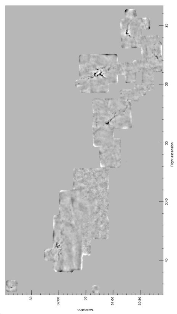
Figure 1: 850 $\mu$m observations of the Perseus molecular cloud. The scale bar indicates Jy/beam measured at every pixel.

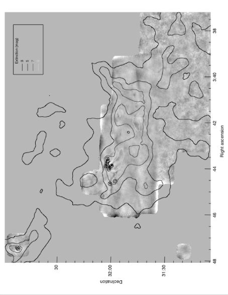
Figure 2: 850 $\mu$m observations of the eastern half of Perseus. Overlaid are contours denoting the extinction (from Alves & Lombardi, 2006, see text for further details). The dark circles indicate where submillimetre clumps were identified (see §3). The scale bar indicates Jy/beam measured at every pixel.

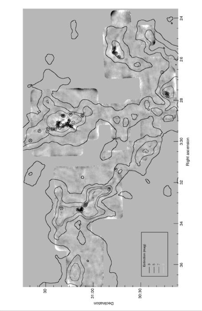
Figure 3: 850 $\mu$m observations of the western half of Perseus. Overlaid are contours denoting the extinction in magnitudes (from Alves & Lombardi, 2006, see text for further details). The dark circles indicate where submillimetre clumps were identified (see §3). The scale bar indicates Jy/beam measured at each pixel.

The resulting map is shown in its entirety in Figure 1, and Figures 2 and 3 show detail of the eastern and western halves of the surveyed cloud.

The extinction data we present here were derived from the Two Micron All Sky Survey (2MASS) images of Perseus by Alves & Lombardi (2006) (see also Ridge et al., 2006b) using the NICER technique (Lombardi & Alves, 2001) as a part of the COMPLETE Survey (Goodman, 2004). The resolution in the Perseus extinction map is $\sim$2.5′ which has the effect of smoothing out the small scale structure in the map and diluting regions of high extinction. Very compact regions of high extinction could be missed entirely if there is an insufficient number of background stars detected to contribute significantly to the extinction calculation. Although the NICER technique utilizes procedures to remove embedded and foreground stars from the extinction derivation, this is difficult, and any still included can introduce errors and affect the observed cloud morphology. The extinction data are denoted by contours overlaid on Figures 2 and 3. It should be noted that Schnee et al (2005) have shown that the extinction determined for a region is uncertain at the 0.2 mag level – a comparison between extinction derived using the NICER technique with 2MASS data and re-reduced IRAS far-IR data showed this point-to-point difference even when optimal cloud-specific dust properties were used.

3 Identification of Structure

We identify structure in both the submillimetre and extinction data, as described in the following subsections.

3.1 Submillimetre Continuum

To identify structure in the 850 $\mu$m map, we used the automated routine Clumpfind (2D version; Williams, de Geus, & Blitz, 1994; Johnstone et al., 2000b). Some clump-identifying algorithms assume a pre-determined shape for the structure (typically Gaussian), leading to the artificial division of more complex objects. Clumpfind, however, does not assume a shape and instead utilizes contours to determine clump boundaries. Bulk clump properties such as the clump mass distribution have been shown to be similar to those found assuming a Gaussian profile for clumps (Johnstone et al., 2000b). With Clumpfind, we identify 58 submillimetre clumps down to a level of 3 times the mean pixel noise. Spurious objects that were either smaller than the beam or noise spikes appearing in regions of higher than average noise, the vast majority of which occur at the map edges, were excluded from this total. Figures 2 and 3 illustrate where these clumps were found. Hatchell et al. (2005), hereafter H05, have recently published a similar analysis on much of the same region of Perseus using a different method for the data reduction and the identification of clumps, and our analysis shows good agreement with their results. The H05 clumps tend to have slightly higher peak fluxes, as the final submillimetre map presented in that paper was neither flattened nor smoothed. Note that a larger number of clumps were identified in H05, as the clump-detection threshold was lower in their analysis (see discussion in $\S 4.1$). Table 1 lists the properties of the clumps we identify, along with the corresponding designations from H05.

The total flux of each clump can be converted into mass assuming that the emission is optically thin and its only source is thermal emission from dust. Following Johnstone et al. (2000b), the conversion is

$${\rm M_{clump}=0.23\ S_{850}\left(\exp\Big{(}\frac{17~{}K}{T_{d}}\Big{)}-1\right)\ \Big{(}\frac{\kappa_{850}}{0.02~{}cm^{2}~{}g^{-1}}\Big{)}^{-1}\ \Big{(}\frac{D}{250~{}pc}\Big{)}^{2}\ M_{\odot}}$$ (1)

where S₈₅₀ is the total flux at 850 $\mu$m, T_d is the dust temperature, $\kappa_{850}$ is the dust opacity at 850 $\mu$m, and D is the distance. Following the Spitzer c2d team (Evans et al., 2003), we adopt a distance of 250 ($\pm$ 50) pc to the Perseus molecular cloud as found by ${\rm\breve{C}}$ernis (1993) and Belikov et al. (2002). A range of distances have been estimated for the Perseus molecular cloud ranging from 350 pc (Herbig & Jones, 1983) to 220 pc (${\rm\breve{C}}$ernis, 1990), with several authors suggesting that the system is composed of two distinct clouds at different distances - e.g., Ungerects & Thaddeus (1987); Goodman et al. (1990); ${\rm\breve{C}}$ernis & Straizys (2003); Ridge et al. (2006a); with the closer cloud being an extension of Taurus and the further a shell-like structure. We also take a typical internal temperature of 15 K and, following Johnstone et al. (2006), a dust opacity of $\kappa_{850}$ = 0.02 cm² g^-1. Therefore, the conversion factor between Jy and M_⊙ is 0.48. H05 adopt values of D = 320 pc, T = 12 K, and $\kappa$ = 0.012 cm² g^-1; thus our masses need to be multiplied by a factor of 4.1 to be compared to the H05 values. The final masses may be scaled by a factor ranging from $\sim$0.3 to 6 given the uncertainties in distance, dust opacity, and clump temperature.

In Table 1, we estimate the number density for each clump using the effective clump radii found by Clumpfind, suggesting that temperatures of tens of Kelvin are required for only thermal support, assuming ${\rm T_{dust}=T_{gas}}$.

3.2 Extinction

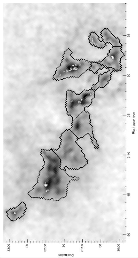
Figure 4: Large scale structure (‘super cores’) identified in extinction data. The scale bar indicates extinction at each point in magnitudes. The white circles indicate the locations of submillimetre clumps identified (see text for details).

Structure also exists in the extinction maps (see Figs 2 and 3). In our submillimetre data, the majority of clumps were isolated, allowing for easy identification of structure. In the extinction map, however, the structure has a large filling factor, making identification and separation much more difficult. Visually, structure is apparent on two scales - a smaller scale consisting of compact objects and a larger scale consisting of groups of the compact objects within a diffuse background. Here, we term these two types of structures as cores and super cores. The extinction level in the diffuse regions of super cores is varied so that a simple utilization of the Clumpfind algorithm does not produce reliable structure identification. To define the larger extinction ‘super cores’, we smoothed the data to 5′ resolution and then ran Clumpfind. The resulting identifications are shown in Figure 4. The smaller extinction ‘cores’ are shaped more regularly, and we found them to be well fit by 2D Gaussians. Although fitting to a Gaussian does have the disadvantage of assuming a shape for the structure, this procedure allows for a separation between diffuse background extinction (associated with the larger extinction super core structure) and the concentrated extinction in the core region. Figure  5 shows the Gaussian models of the extinction cores (excluding the background level).

To convert the extinction measures into mass, we adopt a conversion factor of $<N(H_{I}+H_{2})>/E_{B-V}=5.8\times 10^{21}$ atoms cm^-2 mag^-1 (Bohlin et al., 1978) and a standard reddening law where A_V / E_B-V = 3.09 (Rieke & Lebofsky, 1985). Thus an A_V = 1 mag corresponds to a column density of 1.88 $\times 10^{21}$ (H_I+H₂) cm^-2, or 4.40 $\times 10^{-3}$ g cm^-2 adopting the standard mean molecular weight $\mu$ = 1.4 (Allen, 1973). We find the total mass in the extinction map is ${\rm\sim 1.9\times 10^{4}~{}M_{\odot}}$ (${\rm\sim 6\times 10^{3}~{}M_{\odot}}$ in the region for which we have submillimetre data). Previous extinction mass estimates using the Palomar Sky Survey and mapping in CO have resulted in similar values - Bachiller & Cernicharo (1986) estimate 1.2$\times 10^{4}$ M_⊙ (1.7$\times 10^{4}$ M_⊙ with their assumed distance of 300 pc), while Carpenter (2000) estimate $\sim$ 0.8 $\times 10^{4}$ M_⊙ (1.3$\times 10^{4}$ M_⊙ with their assumed distance of 320 pc) from Padoan et al. (1999)’s observations and H05 estimate $\gtrsim 0.6\times 10^{4}$ M_⊙ ($\gtrsim 10^{4}$ M_⊙ with their assumed distance of 320 pc).

Tables 2 and 3 show the properties of the cores and super cores. We calculated their number density using the half width half max from Gaussian fitting and mean radius derived from the total areal coverage respectively, and find temperatures of over 50 K are required for purely thermal support, which is unrealistic.

4 Mass Distribution

Previous (sub)millimetre studies of star-forming regions (e.g., Motte et al., 1998; Johnstone et al., 2000b, 2001, 2006; Reid & Wilson, 2005; Enoch et al., 2006) have shown that clumps have a mass distribution well fit by a broken power law, with the number of clumps with mass above M, N(M) $\propto$ M^-α. The slope $\alpha$ is similar to or higher than that which characterizes the stellar Initial Mass Function ($\alpha\sim$ 1.35; Salpeter, 1955), with a turnover to a shallower power law at low masses. The turnover observed in the submillimetre tends to occur where incompleteness in the clump sample becomes significant. The similarity between the clump and initial stellar mass functions is suggestive of a direct link between the two, although there are several concerns with this. The total submillimetre clump mass often exceeds that expected to be in the final stars (see Larson, 2005, for a review). This difference might be acounted for through inefficient star formation (e.g., if all clumps lost some percentage of the clump mass reservoir to outflows during formation). A second problem is that there is no evidence that all clumps do form stars. In the turbulent support framework, a significant number of clumps in fact re-expand (e.g., Vázquez-Semadeni et al., 2005). In most cases, there is insufficient data to determine whether the clumps are gravitationally bound. Many theories have been put forth to account for the rough invariance of the slope including turbulent fragmentation (e.g., Padoan & Nordlund, 2004), competitive accretion (e.g., Bonnell, 2005), and thermal fragmentation (e.g., Larson, 2005).

On larger scales within molecular clouds, CO observations have shown that structures follow a mass distribution where the bulk of the mass is contained in the most massive structures (unlike the submillimetre clumps), with a lower value for $\alpha$, between 0.6 and 0.8 (Kramer et al., 1998). The cause for the difference between the large and small scale mass distributions is unknown. It may be due to different methods of observations, in the definition of structure, the effects of chemistry such as freeze-out, or to real differences in the structures at the large and small scales due to the different physical processes that are responsible for fragmentation.

4.1 Submillimetre Continuum

Adopting a common dust temperature of 15 K, we find the submillimetre clumps in Perseus are well fit by a broken power law with $\alpha\sim 2$, which falls within the range of slopes found by previous authors, varying from $\alpha\sim$ 1 - 1.5 (Johnstone et al., 2000b) to $\alpha\sim$ 2 (Reid & Wilson, 2005). Using the temperatures calculated from Bonnor-Ebert modelling (§5), the slope appears to be similar. A recent study of clumps identified at 1.1 mm in Perseus covering 7.5 sq. degrees (Enoch et al., 2006) identified 122 objects and found a mass distribution with a similar slope to the one we find, but includes higher mass objects that belong to more extended structures than our chopped 850 $\mu$m data are sensitive to. We find the mass distribution turns over to a power law with a shallow slope at around 0.3 M_⊙, approximately where our sample begins to suffer from incompleteness. Incompleteness becomes important in our sample where clumps have peak fluxes too low to be identified by Clumpfind. Clumpfind identified objects down to a peak of 5 $\sigma$ and extends them to the 3 $\sigma$ level. Taking a ‘typical’ clump extent of $2.6\times 10^{-3}$ pc² (1800 arcsec²), clumps of masses $\sim$ 0.2 to 0.3 M_⊙ would be missed. H05 identify clumps to a lower central flux (i.e., a lower cutoff) and thus find more sources. Our 1.3 sq. deg of fast-scan observations have a higher noise level than the public archival data analyzed in both papers and we set our Clumpfind threshold higher to reflect this difference.

4.2 Extinction

We also examined the mass distributions of the extinction cores and super cores (see Figure 7). The extinction cores have a similar mass distribution to the submillimetre clumps, with slope of $1.5\leq\alpha\leq 2$ at the high mass end and a turnover at $\sim$40 M_⊙ while the super cores have a shallower mass distribution, similar to that seen from CO data, with a slope of $\alpha\sim 1$. The small numbers of cores and particularly super cores lead to greater uncertainties in the derived slopes. Incompleteness is difficult to quantify accurately for the extinction data, given the methods used for clump identification. The extinction super cores identified comprise virtually all of the mass in the extinction map at A${}_{V}\geq$ 3. At A${}_{V}<3$, the extinction is diffuse and unassociated with any apparent extinction structure. Thus it is likely that sources of additional mass have not been missed throughout the majority of the mass range of identified super cores. Each of these structures, however, may be more massive than estimated. The Gaussian fitting routine for the extinction cores did not fit all of the extinction above A_V = 3, and thus we expect incompleteness at the lower end of the mass distribution. The Gaussian fitting routine models maxima in the extinction map (i.e., peak plus background level); we stopped our search at $\sim$5 mag, or a peak of $\sim$3 mag. Typical core extents are $\sigma_{G}\sim$ 300′, which corresponds to a mass of $\sim$50 M_⊙. Thus the turnover we observe at $\sim$40 M_⊙ is probably not real.

The change in behaviour of the extinction core and super core mass distributions and their close correspondence to the two regimes previously observed in the submillimetre and CO is intriguing. It is possible that the differences are a result of some bias that we introduced through these definitions of the two sets of objects. Projection effects may also play a role in the mass distribution measured. Most of the cores and super cores are bounded by similar objects (unlike the submillimetre clumps), making overlap for the real 3D objects probable. This may have a greater effect on the super cores which are less regularly shaped and larger. Overlap would lead to larger numbers of massive objects (i.e., a shallower slope). With the above caveats, if the slopes are truly different for the cores and super cores, this may be an indication of the scale over which fragmentation changes from a top-heavy to a bottom-heavy mass function due to the importance of different physical processes.

5 Bonnor-Ebert Modelling

To gain further physical insight into the nature of the clumps, we model them as Bonnor-Ebert (BE) spheres – spherically symmetric structures that are isothermal, of finite extent, and bounded by an external pressure, where gravity is balanced by thermal pressure (Bonnor, 1956; Ebert, 1955; Hartmann, 1998). Previous work (e.g., Alves et al., 2001; Johnstone et al., 2000b, 2001, 2006) has shown that submillimetre clumps can be well fit by a BE sphere model. Each BE sphere is parameterized by its central density, external pressure, and temperature, each of which can be extracted from a best fit to the data.

Recent work has shown that caution is needed in the interpretation of the fit to a BE sphere model, as dynamic entities produced in turbulent simulations can mimic the column density profile of a stable BE sphere (Ballesteros-Paredes et al., 2003). BE sphere models are useful, however, in illustrating the minimum level of support that would be necessary to prevent collapse in an object of given mass and radius bounded by a finite pressure.

BE spheres are characterized by a one-dimensional radial density profile, with a family of models defined by each dimensionless truncation radius. Each family of BE spheres possesses a unique importance of self-gravity, or equivalently the central concentration of a clump, with a higher concentration corresponding to a higher importance of self-gravity. Each concentration therefore defines a unique family of BE spheres. Following Johnstone et al. (2001), we define the concentration to be (in terms of observable quantities)

$${\rm C=1-\frac{1.13\,B^{2}\,S_{850}}{(\pi R^{2}_{obs})\,f_{0}}}$$ (2)

where B is the beamsize, S₈₅₀ is the total flux, $\rm R_{obs}$ the radius, and f₀ the peak flux. The concentrations are approximate due to the relatively large size of the beam compared with the clump radius as well as projection effects. To be fit by the Bonnor-Ebert sphere model, the concentration must be greater than 0.33 (corresponding to a uniform density sphere) and less than 0.72 (Johnstone et al., 2000b). To be stable from collapse, clumps with concentrations above 0.72 require additional support mechanisms (for example, pressure from magnetic fields). Alternatively, these high concentration clumps may be more evolved and already experiencing collapse. Walawender et al. (2005) and Walawender et al. (2006) analyzed multiwavelength data in the B1 core of Perseus and found that all clumps with concentrations above 0.75 contained protostars, while none of those at low concentrations ($<$ 0.4) and few at the intermediate concentrations did. Concentration thus appears to be a good indicator of time evolution.

We use the concentration to fit the clumps to stable Bonnor-Ebert spheres following Johnstone et al. (2006), again adopting a distance of 250 pc and an opacity of 0.02 cm² g^-1. Non-thermal support may exist in the clumps. Goodman et al. (1998) find in their survey of prestellar cores that non-thermal support levels are a non-negligible fraction of the thermal support level. Following Johnstone et al. (2006), we assume an equal level of thermal and non-thermal support. Comparable levels of thermal and non-thermal support may not be the case everywhere. Tafalla et al. (2004) show that non-thermal support is negligible in the cores in the quiescent star-forming region Taurus. A lower level of non-thermal support would increase our best-fit temperatures.

Our best fits include temperatures ranging from 10 K to 19 K and external pressures within 5.5 $\leq$ log₁₀(P/k) $\leq$ 6.0 (see Table 1). The physical properties fit to clumps with concentrations outside the stable range are less reliable. The external clump pressures found with the BE modelling are in the range expected to be generated by the pressure due to the weight of the surrounding material in the molecular cloud. For example, the pressure due to overlying material can be written as ${\rm P/k=1.7\times 10^{4}~{}\overline{A}_{V}A_{V}~{}cm^{-3}~{}K}$, where the mean extinction is $\sim$2.2 mag (see §6) and thus the mean pressure in the molecular cloud is log₁₀(P/k) $\approx$ 4.9. The highest extinction in the cloud is 11.8 mag, corresponding to a central pressure in the cloud due to the surrounding material of log₁₀(P/k) $\approx$ 5.6. Higher pressures can be generated by the extra weight of material in large cores with local mean extinctions higher than 2.2 mag. The pressures fit here are lower than those found by Johnstone et al. (2000b) in the Ophiuchus molecular cloud (they found 6 $\leq$ log₁₀(P/k) $\leq$ 7), consistent with the fact that the total column densities (or extinctions), and hence pressures found in Ophiuchus are larger – Johnstone, Di Francesco, & Kirk (2004) (hereafter JDK04) found a mean extinction of 4 mag and a peak extinction of 35 mag.

The temperatures derived from the Bonnor-Ebert fits provide a second estimate of the clump masses (also included in Table 1), as discussed in Section 4. These clump masses correspond closely to those calculated assuming a constant temperature of 15 K, indicating that the temperature assumed should not be of critical importance to the further analysis presented.

6 Clump Environment: Extinction Threshold

Following JDK04, we examine the relationship between the locations of small-scale, submillimetre clumps relative to the overall cloud structure traced by extinction. Figure 8 shows the cumulative mass in the submillimetre clumps and extinction map at increasing A_V. Table 4 includes the fraction of the submillimetre clumps and extinction data within three bins of extinction. These demonstrate that most of the mass of the cloud lies at low extinction – 58$\%$ at A${}_{V}\leq$ 5 – the submillimetre clump mass is biased towards the high extinction regions and only a small fraction (1$\%$) is found at A${}_{V}\leq$ 5. Very little of the mass of the cloud is at high extinction – 1$\%$ at A${}_{V}\geq$ 10, while 13$\%$ of the submillimetre clump mass is found there. The portion of Perseus for which we have submillimetre observations is in itself biased towards higher extinctions - the extinction data of the entire region of Figure 1 suggest 86$\%$ of the mass of the cloud is at A${}_{V}<$ 5 and a mere 0.4$\%$ at A${}_{V}>$ 10.

These data suggest small scale structure and hence stars are able to form only at higher extinctions and here we argue that this is not an observational bias. We model the effect of lower extinction (and therefore lower external pressure) on the observability of clumps using the BE sphere model, following the procedure of JDK04.

We use the extinction as a measure of the local pressure and determine how a model clump’s observable properties would be expected to vary with extinction for a given importance of self-gravity (or equivalently concentration, C) assuming it to be a BE sphere. Following McKee (1989), the pressure at depth r is P(r) = ${\rm\pi G\overline{\Sigma}\Sigma}(r)$ where $\overline{\Sigma}$ is the mean column density and $\Sigma(r)$ the column density measured from the cloud surface to depth r. Near the centre of the cloud, $\Sigma(r)\simeq\Sigma(s)/2$, where $\Sigma(s)$ is the column density through the cloud at impact parameter s. The extinction can be expressed as ${\rm A_{V}=(\Sigma/\Sigma_{0})}$ mag where ${\rm\Sigma_{0}=4.68\times 10^{-3}~{}g~{}cm^{-2}}$ (McKee, 1989). The pressure in the cloud at depth r can then be approximated as P($r$)/k = 1.7${\rm\times 10^{4}\overline{A}_{V}A_{V}}(s)~{}{\rm cm^{-3}~{}K}$, where ${\rm\overline{A}_{V}}$ is the mean extinction through the cloud (which we take to be 2.2 mag) and ${\rm A_{V}}(s)$ is the extinction through the cloud at impact parameter s. For a given concentration, the mass and radius of a BE sphere scale as ${\rm M_{BE}\ \propto\ P^{-1/2}}$ and ${\rm R_{BE}\ \propto\ P^{-1/2}}$ (Hartmann, 1998), and thus the column density scales as ${\rm\Sigma_{BE}\ \propto\ P^{1/2}}$. If we assume a constant temperature and dust grain opacity, then for a given concentration, observable clump properties scale as follows – ${\rm S_{850}\ \propto\ A_{V}}(s)^{-1/2}$, ${\rm f_{0}\ \propto\ A_{V}}(s)^{1/2}$, and R ${\rm\propto\ A_{V}}(s)^{-1/2}$, where S₈₅₀ is the total flux, f₀ is the peak flux, and R the radius. All three quantities increase with increasing concentration.

Figure 9 plots these quantities versus the local extinction. The dotted line illustrates the BE model relations for a concentration matching the observed clumps at A_V = 5. The lack of clumps at lower $A_{V}$ is incompatible with our detection of clumps at higher $A_{V}$, suggesting an extinction threshold in clump formation. If all of the submillimetre clumps detected are considered, the extinction threshold appears to be at A${}_{V}\sim$ 5. If we ignore the clumps in L1448 (non-asterisked diamonds), however, we find an extinction threshold at A${}_{V}\sim$ 7. L1448 (extinction core #38) is unusual in that it is within the only extinction core with a low value of peak extinction that contains submillimetre clumps. Previous studies have shown that L1448 contains several very powerful outflows which contain at least as much momentum as that found in the quiescent cores in the region (estimated from the mass and small turbulent velocity of the cores) and more energy than the gravitational binding energy of the region (Wolf-Chase et al., 2000). If there is a mechanism in place for transferring some of the momentum and energy into the surrounding core material, much of that material would dissipate, leading to the lower peak exinction observed in the region. To include consideration of this possibility, we denote its associated clumps with a different symbol in the extinction threshold analysis to allow considerations both with and without them. In the rest of our analyses, we find the submillimetre clumps in L1448 exhibit similar properties to those in other cores. A similar argument for advanced evolution might also be put forth for the NGC1333 region, well known for its active star formation and numerous protostellar outflows. Here, we merely note that the extinction properties of submillimetre clumps within the L1448 core appear different from the other extinction cores and offer the above evolution argument as a possible reason for this difference.

The archival submillimetre data included in the present analysis were also examined by H05 who compared them with C¹⁸O observations to measure the large scale structure of the cloud and search for a column density threshold. H05 examined the distribution of submillimetre clumps (identified through a contouring procedure rather than Clumpfind) with respect to the background column density inferred from C¹⁸O in terms of a probability distribution weighted towards how frequently each column density occurs in the map. They found a sharply decreasing likelihood of submillimetre clumps at lower extinctions, but a non-zero probability for their lowest extinction bin. The sharp decrease in probability is in agreement with the results we present in Table 4, although H05 find ten clumps at A${}_{V}<$ 5.2, contrary to our results (we identify two, which may be noise). Generally, our clumps do correspond well to those found by Hatchell et al., with the differences mainly due to definitions of clump boundaries and identification thresholds which are not easily comparable given the different data reduction methods. Our two clumps at low extinction corresponds to two of their ten. A further two of the ten do not correspond to any submillimetre clumps in our map. These two unmatched clumps are located in regions where there is no submillimetre structure in our map above the threshold we set for identification and visually there appears to be only noise features. The isolation of these two clumps from regions containing the bulk of the clumps coupled with the lack of visible submillimetre structure in our map further suggests that these are noise features. The remaining six clumps are located in regions where we see clumps, but the extinction we measure at these locations is much higher than found by H05 (two clump locations are at 5.5 - 6 mag, while the other four are around 8-9 mag in our map). The majority of the disagreement in clump identification at low column densities is due to the different methods of calculating column density and extinction. Our method (using extinction from 2MASS) is less prone to chemical effects such as freeze-out at high densities or photodisociation at the cloud edge which could effect H05’s C¹⁸O map and arguably produces a more accurate count of the total column density of material along the line of sight, although our data does have lower resolution (2.5′ vs 1′). Furthermore, our extinction map includes any foreground dust along the line of sight and could be distorted by young embedded protostars (see discussion in §2). We note that Enoch et al. (2006) found an extinction threshold of $\sim$5 mag in their analysis of 1.1 mm observations of the Perseus molecular cloud.

Column density or extinction thresholds for star formation have been found in other regions. For example, our previous work (JDK04) used the same method of analysis as outlined above to argue that an extinction threshold of A${}_{V}\sim 15$ exists in the Ophiuchus molecular cloud. In addition, Onishi et al. (1998) analyzed C¹⁸O observations of the Taurus molecular cloud in combination with IRAS data and argued that recently formed protostars (“cold IRAS sources”) are found only in regions with a column density of N(H₂) $>8\times 10^{21}~{}{\rm cm}^{-2}$, corresponding to an A_V of $>$ 4 (adopting the conversion factor used in this paper; §3.2), and that all regions with column densities above this threshold contain ‘cold IRAS sources’, suggesting that once the critical column density is reached, formation occurs quickly. In contrast, we find several extinction regions (cores #11, 20, and 25 or super core #4) in Perseus above our extinction threshold of A_V = 5 that do not contain any submillimetre clumps. This may be a reflection of the different environment in which stars form in the two clouds, or it may an observational effect (i.e. sensitivity or the definition of cores). No objects from the IRAS point source catalog lie within the empty super core #4, although counterparts to the lowest flux objects in Taurus could be missed since Taurus is roughly three-fifths as distant as Perseus (140 $\pm$ 10 pc; Kenyon et al., 1994). We also do not see any hint of submillimetre clumps in the empty super core, even below our detection threshold, implying that any clumps present would not be comparable to those observed in the other cores in Perseus. The definition of extinction cores is another possibility for an observational difference between the Taurus and Perseus surveys. The angular resolutions are comparable (the Onishi et al. maps have a beamsize of 2.7′, while our extinction maps have a resolution of 2.5′) so the Taurus extinction cores could be further subdivided on a physical scale, however, chemical processes such as freeze-out could make the CO distribution smoother and hence less clumpy. Empty super core #4 (which contains core #20), however, appears to be rather isolated and it is unlikely that a smoothing effect would result in a substantial change in its definition.

An extinction threshold is a natural consequence of the magnetic support model. Under this model, dense clumps become gravitationally unstable through ambipolar diffusion. The ambipolar diffusion timescale is a function of the density of ions in the region and only becomes short enough to be significant for higher extinctions where cosmic rays are the sole source of ionization. In particular, McKee (1989) argues for an extinction threshold between 4 and 8 mag, the exact value depending on the density of the cloud and the characteristic density in which cosmic rays dominate the ionization process. Cloud geometery and the strength of the local interstellar radiation field also play a role in the column density threshold observed. The extinction thresholds observed in Perseus and Taurus are easily consistent with that predicted by the magnetic support model. Given the effect of geometry, etc., the Ophiuchus results also appear to be consistent, as argued by JDK04. Further research is required to determine if the turbulent support model is able to provide an explanation for an extinction threshold.

7 Triggered Star Formation

Figure 10 illustrates how the submillimetre clumps are preferentially located offset from the peak of their parent extinction core (see also Figure 11 for a close-up of the distribution of submillimetre clumps within each extinction core). The difference in resolution between the two data sets is substantial ($\sim$20″ vs. 2.5′), but this is not the cause of the offset in peak positions. For example, we smoothed the submillimetre data to a resolution of 2.5′ and found that the offset still remained. The offsets across extinction structure furthermore appear to be correlated, as discussed in more detail below. One would expect, from simple models of either magnetic or turbulent support, for clumps to preferentially form in the densest regions. While our observations are only able to demonstrate that the submillimetre structure is offset from the peak column density, it is difficult to imagine a scenario where geometrical effects alone produce the correlation in submillimetre clump offsets while having no relation to offsets in the underlying density distribution. Thus, the submillimetre offsets suggest an additional mechanism to magnetic or turbulent support may be at work. The correlation between the submillimetre clump offsets from the peaks in each extinction core over our entire map suggests the importance of an outside agent in clump formation or evolution.

A triggered formation scenario for the Perseus molecular cloud has been previously suggested by Walawender et al. (2004). There, infrared observations of a cometary cloud in the L1451 region (to the southwest of our map), that appears to be eroding by UV radiation, led to the suggestion that the B0.5 star 40 Persei, of the Perseus OB assocation, is a likely candidate for triggering star formation in that region. The small-scale (‘globule-squeezing’) formation scenario is also consisent with our observations of Perseus as a whole. For example, UV radiation from members of the OB association could erode and heat the surfaces of extinction cores on the side facing the radiation, leading to a triggering of the evolution of pre-existing structure on that side of the core.

A moderate temperature gradient across the extinction structures caused by incoming UV radiation is likely insufficient to explain the visibility of submillimetre clumps solely on one side of the extinction cores. Submillimetre clumps are detected with fluxes an order of magnitude above the 3$\sigma$ noise level. Temperatures differing by factors of more than four would be required to explain the non-detections versus detections on opposing sides of the core. This is unlikely to be the case as our BE models suggest that the clumps we detect have temperatures of $\sim$15 K, and thus any equivalent population of undetected submillimetre clumps would be at temperatures of $\sim$4 K.

The vectors in Figure 10 indicate the direction of 40 Per from each of the relevant extinction cores, illustrating that while the correspondence between the clump locations and the direction to 40 Per is not perfect, the two are in good agreement especially given that we are only viewing a 2D projection the region. We can quantify the agreement between submillimetre clump locations and the scenario of 40 Per as a trigger as follows. Assuming (for simplicity) that all the extinction cores were spherical, we would expect that triggering would take place where incident radiation from 40 Per hits the core, i.e., within $\pm$ 90° of the separation vector between the extinction core and 40 Per. Here we will refer to the angle that clumps are offset from the separation vector between their parent extinction core centre and 40 Per as the clump angle. Examining our submillimetre clumps, we find that 78$\%$ have clump angles within the $\pm$ 90° boundary and 86$\%$ within $\pm$ 100°, with an average clump angle of -11° (see Figure 12 for the distribution). Several clumps have angular separations well outside the $\pm$ 90° range - all of these are located in the western portion of the map where the extinction core geometry is more complex. These clumps may be more poorly described as associated with their Gaussian model extinction core, or otherwise require three dimensional geometry to fully understand them. The distribution of clump angles is generally in agreement with 40 Per as a candidate trigger, but does not necessarily rule out other potential trigger candidates. A trigger source nearby 40 Per would be expected to give a similar distribution of clump angles over a range of extinction cores, but with clumps in cores westward of 40 Per having preferentially negative clump angles and clumps eastward of 40 Per having preferentially positive clump angles, or vice versa. We examined the distribution of clump angles for those eastward and westward of 40 Per and do not observe such a skew (see Figure 12). Clumps eastward of 40 Per have an average clump angle of 13° to 40 Per and clumps westward of 40 Per have an average clump angle of -19° to 40 Per, but the overall distributions do not appear to be skewed, and the difference in the averages may in part be due to small number statistics. Thus 40 Per appears to be the likely trigger, though any nearby (similar angle from the cloud) sources are not ruled out. Other possibilities for this geometric coincidence exist such as clump motion from the parent extinction core caused by stellar wind pressure perhaps from a source such as 40 Per.

We note that the ring observed in ¹³CO measurements of the Perseus molecular cloud as a part of the COMPLETE survey (Ridge et al., 2006a) appears to be unrelated to any triggering event due to its location (Figure 10). This is consistent with the Ridge et al. (2006a) results that the ring appears to be behind the bulk of the cloud.

One outstanding puzzle is the extinction cores which show no evidence of clumps, especially the ones with significant portions above the extinction threshold (#11, 20, 25) as discussed earlier (Section 6). The three dimensional geometry of the extinction cores is not known, but this could explain the lack of submillimetre clumps seen in these ‘empty’ extinction cores. Shielding by a large column of cloud material separating the empty extinction cores from the trigger is possible. Higher signal to noise observations of the ‘empty’ extinciton cores may reveal submillimetre clumps, but any such clumps would possess a lower mass and central density than the clumps presented here. This would still lead to the question of why two extinction cores with similar peak extinctions would develop different populations of submillimetre clumps. Higher sensitivity observations of the ‘empty’ extinction cores (especially extinction core #20 which does not lie within a larger super core in which clumps are observed) are required to understand what processes make them different. Spitzer c2d observations of these regions should provide some clue to their protostellar content.

8 Conclusions

We present an analysis of 3.5 square degrees of submillimetre continuum data and the corresponding extinction map of the Perseus molecular cloud. We identify structure in both maps of submillimetre emission (clumps) and extinction (cores and super cores). The cumulative mass distribution of all three sets of structures are well characterized by broken power laws. The submillimetre clumps and extinction cores have high-end mass distribution slopes of $\alpha\sim 2$ and 1.5 - 2 respectively. These are slighly steeper than the Salpeter IMF ($\alpha\sim$ 1.35), but within the range found in submillimetre clumps in other star forming regions. In contrast, the mass distribution of extinction super cores is best fit by a shallow slope of $\alpha\sim 1$, corresponding to slopes observed in structures identified in large scale CO maps. The difference between the extinction cores and super cores may be an observational bias or it may indicate the scale over which different processes become important in fragmentation.

The majority of submilimetre clumps can be well fit by a Bonnor-Ebert sphere model of equal thermal and non-thermal internal pressure, with external pressures ranging from ${\rm 5.5<\ \log_{10}(P_{ext}/k)<6.0}$ and temperatures ranging from 10 to 19 K. The derived pressures are comparable to the pressures expected to be exerted by the weight of the surrounding cloud material and the temperatures fall within the range expected for a molecular cloud.

We show that small scale (submillimetre) structure (clumps) is located only in regions of high extinction. Submillimetre clumps are found only at A${}_{V}~{}>$ 5 - 7, although BE models suggest that we should have been able to detect clumps at lower A_V had they existed. In turn, this suggests that clumps are only able to form above a certain extinction level. An extinction threshold is consistent with the model of magnetic cloud support, where the timescale for ambipolar diffusion is only of a reasonable length in regions above an A_V of 4 - 8 mag. It is less clear if the turbulent support model can explain our observations.

The submillimetre clumps were preferentially found offset from the peaks of several extinction cores. The correlation of these locations suggests a small-scale triggering event formed the submillimetre clumps in the region. Furthermore, the position of the young B0 star 40 Per, previously suggested as a source of triggering for the region by Walawender et al. (2004), coincides with the expected position of a triggering source.

Large-scale submillimetre surveys, such as the one presented here, will become practical to carry out on a large number of molecular clouds with SCBUA-2, a bolometer array to be installed at the JCMT in late 2006. SCUBA-2 will have a higher sensitivity and a larger field of view than SCUBA, allowing large areas to be mapped up to 1000 times faster than using SCUBA. Legacy surveys have been approved, including the Gould’s Belt Survey, in which nearby molecular clouds will be mapped in their entirety (A${}_{V}>$ 1) in submillimetre continuum, as well as more focussed complimentary observations of molecular line emission and polarimetry. These will enable a comprehensive study of the large scale environment of molecular clouds, allowing a determination of the importance of the cloud support mechanisms.

9 Acknowledgements

We thank Joao Alves and Marko Lombardi for providing the extinction data as well as fruitful discussions on its interpretation. We would also like to thank Jenny Hatchell for allowing us to see the data presented in her paper before publication. We are also grateful for the helpful comments provided by the referee, Alyssa Goodman.

HK is supported by a Univeristy of Victoria Fellowship and a National Research Council of Canada GSSSP Award. DJ is supported by a Natural Sciences and Engineering Research Council of Canada grant.

Table 1: Properties of submillimetre clumps in Perseus.

Name	RA	Dec	f0	S850	Reff	Mass	Conc	Temp	MBE	log $n_{cent}$	log Pext/k	H05	Extinction
(SMM J)	(J2000.0)	(J2000.0)	(Jy/bm)	(Jy)	(″)	M⊙		(K)	M⊙	cm-3	cm3 K-1	#	Core #
034769+32517	3:47:41.6	32:51:48.0	0.29	0.60	23.	0.3	0.45	12.	0.54	5.2	5.9	78	1
034764+32523	3:47:38.8	32:52:18.9	0.25	0.61	26.	0.3	0.48	10.	0.66	5.2	5.8	79	1
034472+32015	3:44:43.7	32:01:32.3	0.44	0.76	24.	0.4	0.56	10.	0.84	5.5	5.9	14	5
034461+31587	3:44:36.8	31:58:46.1	0.18	0.30	19.	0.2	0.31	14.	0.19	4.9	5.9	19	5
034410+32022	3:44:06.1	32:02:17.7	0.19	0.68	27.	0.4	0.30	17.	0.32	4.6	5.7	22	5
034404+32025	3:44:02.8	32:02:30.5	0.23	0.98	29.	0.6	0.29	18.	0.39	4.6	5.8	18	5
034402+32020	3:44:01.3	32:02:00.8	0.27	0.94	29.	0.5	0.41	14.	0.56	4.8	5.8	16	5
034396+32040	3:43:57.7	32:04:01.6	0.22	0.80	28.	0.4	0.36	17.	0.36	4.6	5.7	17	5
034395+32030	3:43:57.2	32:03:01.8	0.82	2.27	37.	1.3	0.71	12.	1.92	5.6	5.6	13	5
034394+32008	3:43:56.5	32:00:50.0	1.04	3.14	39.	1.7	0.72	13.	2.24	5.7	5.6	12	5
034385+32033	3:43:51.0	32:03:21.2	0.34	1.46	36.	0.8	0.52	12.	1.26	5.1	5.7	15	5
034376+32031	3:43:45.8	32:03:10.4	0.15	0.81	30.	0.4	0.17	17.	0.37	4.5	5.7	–	5
034373+32028	3:43:43.9	32:02:52.9	0.17	0.76	28.	0.4	0.22	17.	0.35	4.6	5.7	26	5
034363+32032	3:43:38.3	32:03:12.1	0.17	0.31	19.	0.2	0.29	14.	0.19	4.8	5.9	23	5
033335+31075	3:33:21.3	31:07:34.6	1.16	5.83	51.	3.2	0.72	15.	3.33	5.5	5.5	2	21
033329+31095	3:33:17.9	31:09:34.3	1.25	4.38	49.	2.4	0.79	13.	2.95	5.5	5.5	1	21
033326+31069	3:33:16.1	31:06:58.2	0.53	4.96	54.	2.8	0.54	15.	2.66	4.9	5.6	4	21
033322+31199	3:33:13.4	31:19:58.0	0.18	0.39	21.	0.2	0.29	15.	0.22	4.8	5.9	82	22
033309+31050	3:33:05.4	31:05:03.4	0.17	0.77	30.	0.4	0.26	17.	0.36	4.5	5.7	6	21
033303+31044	3:33:02.2	31:04:27.1	0.16	1.30	40.	0.7	0.26	18.	0.52	4.3	5.5	5	21
033229+30497	3:32:18.0	30:49:47.1	1.22	2.13	32.	1.2	0.76	12.	1.73	5.8	5.8	76	23
033134+30454	3:31:20.9	30:45:28.4	0.59	0.91	24.	0.5	0.62	10.	0.98	5.7	5.9	77	23
032986+31391	3:29:51.8	31:39:08.0	0.25	0.41	20.	0.2	0.42	12.	0.36	5.1	6.0	–	26
032942+31283	3:29:25.3	31:28:21.2	0.18	0.20	15.	0.1	0.28	13.	0.14	5.0	6.1	64	28
032939+31333	3:29:23.5	31:33:20.8	0.23	0.39	19.	0.2	0.36	15.	0.21	4.8	5.9	58	26
032931+31232	3:29:18.6	31:23:14.0	0.29	0.92	28.	0.5	0.44	12.	0.70	5.0	5.8	63	28
032930+31251	3:29:18.0	31:25:07.8	0.29	1.81	44.	1.0	0.55	11.	1.64	5.0	5.5	57	28
032928+31278	3:29:17.4	31:27:49.7	0.22	0.47	22.	0.3	0.40	13.	0.35	4.9	5.9	61	28
032925+31205	3:29:15.1	31:20:31.3	0.18	0.40	21.	0.2	0.29	15.	0.23	4.8	5.9	70	28
032919+31131	3:29:11.4	31:13:06.7	2.61	6.42	46.	3.6	0.83	16.	3.27	5.6	5.7	42	30
032917+31184	3:29:10.6	31:18:24.5	0.88	3.42	41.	1.9	0.68	13.	2.34	5.5	5.6	46	28
032917+31217	3:29:10.3	31:21:42.4	0.39	1.57	33.	0.9	0.46	14.	1.00	5.0	5.8	54	28
032916+31135	3:29:10.0	31:13:30.4	5.27	8.51	38.	4.7	0.84	19.	3.22	5.9	6.0	41	30
032914+31152	3:29:08.9	31:15:12.2	0.55	1.99	34.	1.1	0.56	13.	1.49	5.3	5.8	51	31
032912+31218	3:29:07.5	31:21:53.8	0.37	1.75	36.	1.0	0.50	13.	1.25	5.0	5.7	56	28
032911+31173	3:29:06.9	31:17:23.8	0.29	1.01	29.	0.6	0.41	15.	0.58	4.8	5.8	62	28
032910+31156	3:29:06.6	31:15:41.7	0.62	2.03	30.	1.1	0.49	15.	1.14	5.2	6.0	50	31
032905+31149	3:29:03.3	31:14:59.1	0.49	2.00	32.	1.1	0.45	16.	1.03	5.0	5.9	52	31
032905+31159	3:29:03.2	31:15:59.0	2.31	6.07	36.	3.4	0.70	17.	2.72	5.8	6.0	43	31
032901+31204	3:29:01.0	31:20:28.5	0.92	5.07	45.	2.8	0.61	16.	2.71	5.3	5.7	45	28
032900+31119	3:29:00.3	31:11:58.5	0.16	0.13	12.	0.1	0.24	12.	0.11	5.2	6.1	65	30
032899+31215	3:28:59.6	31:21:34.2	0.62	2.40	39.	1.3	0.63	12.	1.89	5.4	5.7	47	28
032891+31145	3:28:54.9	31:14:33.4	1.63	4.02	41.	2.2	0.79	14.	2.53	5.7	5.7	44	31
032866+31179	3:28:40.2	31:17:54.3	0.31	1.14	30.	0.6	0.42	14.	0.69	4.9	5.8	55	31
032865+31060	3:28:39.2	31:06:00.3	0.15	0.83	32.	0.5	0.25	17.	0.39	4.4	5.6	75	30
032865+31185	3:28:39.2	31:18:30.0	0.29	1.32	34.	0.7	0.44	14.	0.87	4.8	5.7	60	28
032861+31134	3:28:36.8	31:13:29.6	0.43	0.97	27.	0.5	0.57	11.	1.01	5.4	5.8	49	31
032780+30121	3:27:48.4	30:12:08.7	0.23	0.95	31.	0.5	0.39	15.	0.53	4.7	5.7	37	34
032771+30125	3:27:42.8	30:12:31.4	0.30	1.00	30.	0.6	0.45	12.	0.77	5.0	5.8	36	34
032766+30122	3:27:40.0	30:12:12.7	0.22	0.62	23.	0.3	0.27	17.	0.29	4.7	5.9	40	34
032765+30130	3:27:39.0	30:13:00.4	0.41	0.79	23.	0.4	0.50	11.	0.73	5.3	6.0	35	34
032763+30139	3:27:38.0	30:13:54.2	0.18	0.26	17.	0.2	0.30	14.	0.17	4.9	6.0	39	34
032662+30153	3:26:37.3	30:15:20.8	0.17	0.17	14.	0.1	0.23	13.	0.12	5.1	6.1	80	35
032581+30423	3:25:49.1	30:42:18.1	0.28	1.61	37.	0.9	0.41	16.	0.84	4.7	5.7	32	38
032564+30440	3:25:38.7	30:44:03.0	1.09	2.14	32.	1.2	0.72	12.	1.72	5.8	5.8	29	38
032560+30453	3:25:36.2	30:45:20.2	2.85	8.90	52.	4.9	0.84	17.	4.01	5.6	5.6	28	38
032543+30450	3:25:26.0	30:45:05.2	0.31	1.69	37.	0.9	0.42	16.	0.90	4.7	5.7	31	38
032537+30451	3:25:22.3	30:45:10.0	0.78	1.94	33.	1.1	0.68	12.	1.68	5.7	5.7	30	38

Table 2: Properties of extinction cores in Perseus.

Ref #	RA	Dec	Peak	A0	Mass	$\sigma_{x}$	$\sigma_{y}$	$<$n$>$	Extinction
	(J2000.0)	(J2000.0)	(AV)	(AV)	(M⊙)	(″)	(″)	($10^{3}$cm-3)	Sup. Core #
1	3:47:43.8	32:52:08.0	4.1	2.6	80.3	394.	253.	5.2	6
2	3:47:01.8	32:42:34.9	2.3	2.4	24.8	192.	291.	3.9	6
3	3:44:47.1	31:40:31.6	2.9	3.4	47.8	327.	258.	4.4	2
4	3:44:42.4	32:15:09.2	2.7	2.8	39.2	311.	237.	4.4	2
5	3:43:54.2	31:58:53.4	6.0	3.7	204.9	540.	324.	5.5	2
6	3:43:38.3	31:43:51.3	3.2	4.0	60.0	431.	227.	3.5	2
7	3:43:25.5	31:41:24.2	1.1	3.7	3.4	144.	115.	3.6	2
8	3:43:08.7	31:54:33.6	1.6	3.5	11.7	147.	252.	3.1	2
9	3:42:57.8	31:48:16.5	0.9	3.3	10.9	435.	138.	0.8	2
10	3:42:01.4	31:48:04.8	4.1	4.3	143.5	561.	321.	3.5	2
11	3:41:48.3	31:57:43.0	3.6	3.0	66.3	482.	198.	3.1	2
12	3:41:34.7	31:43:21.4	2.3	2.8	33.2	398.	184.	2.6	2
13	3:40:45.2	31:48:47.0	2.5	4.6	43.3	189.	469.	2.2	2
14	3:40:37.3	31:14:12.6	1.9	3.4	45.6	333.	364.	2.5	7
15	3:40:26.6	31:43:13.5	1.9	3.2	34.7	255.	362.	2.7	2
16	3:40:17.5	31:59:50.6	2.8	2.8	56.0	201.	502.	2.4	2
17	3:40:01.1	31:31:10.8	1.6	3.8	26.8	213.	403.	1.9	7
18	3:39:26.7	31:21:44.6	1.9	4.2	11.4	118.	264.	3.2	7
19	3:37:57.6	31:25:20.6	2.6	2.8	103.3	629.	327.	1.9	7
20	3:36:26.1	31:11:12.6	5.3	3.6	70.9	208.	332.	7.9	4
21	3:33:31.0	31:01:11.3	5.3	2.2	65.8	346.	185.	7.3	3
22	3:33:29.2	31:18:14.1	5.9	2.7	144.7	430.	292.	6.9	3
23	3:32:38.4	30:58:15.4	6.4	2.8	130.9	206.	505.	5.4	3
24	3:32:21.9	31:22:02.1	3.3	2.0	39.1	268.	226.	6.1	3
25	3:30:27.9	30:26:38.5	4.5	1.9	116.6	260.	511.	4.1	8
26	3:29:40.5	31:37:34.4	3.9	2.3	84.5	410.	273.	4.7	1
27	3:29:03.8	30:04:28.1	2.7	2.0	31.9	235.	260.	5.0	5
28	3:28:58.9	31:22:01.0	6.5	3.8	161.9	421.	304.	7.7	1
29	3:28:51.2	30:44:36.1	2.0	2.5	39.4	217.	474.	1.9	11
30	3:28:50.6	31:09:11.5	3.3	3.5	40.9	376.	170.	3.9	1
31	3:28:42.3	31:12:21.7	1.4	3.2	9.7	428.	81.	0.8	1
32	3:28:27.9	30:19:32.0	2.3	2.8	61.2	191.	723.	1.0	5
33	3:27:58.5	31:26:45.5	2.8	2.8	28.9	317.	167.	4.2	1
34	3:27:34.9	30:11:56.4	5.1	3.6	48.9	206.	238.	10.5	5
35	3:27:08.3	30:05:26.3	2.4	2.8	56.1	220.	537.	1.9	5
36	3:26:13.4	30:29:45.7	2.6	2.0	24.0	187.	249.	5.3	10
37	3:25:40.8	30:09:14.3	3.0	1.8	63.7	491.	220.	2.7	9
38	3:25:25.6	30:42:50.1	3.5	2.1	75.6	453.	244.	3.7	10
39	3:24:53.2	30:22:35.0	3.2	2.3	75.9	529.	228.	2.7	9

Table 3: Properties of extinction super cores in Perseus.

Ref #	RA	Dec	Peak	Mass	Reff	$<$n$>$
	(J2000.0)	(J2000.0)	AV	(M⊙)	(″)	$10^{3}$cm-3
1	3:47:45.3	32:52:43.4	10.9	859.6	776.	7.1
2	3:43:57.1	31:59:28.7	10.1	1938.9	1119.	5.3
3	3:39:27.4	31:21:08.6	10.4	780.6	737.	7.5
4	3:36:28.9	31:11:13.1	9.3	560.5	670.	7.2
5	3:32:35.6	30:58:27.7	9.5	441.1	579.	8.8
6	3:30:28.7	30:26:30.2	7.6	257.6	454.	10.6
7	3:28:56.0	31:22:36.4	6.1	973.3	889.	5.3
8	3:28:53.3	30:44:00.5	7.0	246.2	453.	10.2
9	3:27:36.6	30:12:32.8	6.1	240.1	448.	10.3
10	3:25:22.8	30:43:19.2	5.9	173.7	386.	11.6
11	3:24:50.3	30:23:10.1	5.6	107.4	309.	14.0

Table 4: Distribution of mass in the Perseus molecular cloud binned with extinction.

AV	Cloud Area	Cloud Mass		Cloud Mass		Clump Mass		Mass Ratio
Range	($\%$)	M⊙	$\%$	M⊙	$\%$	M⊙	$\%$	($\%$)
0-12	100	18572	100	6094	100	61.3	100	1.0
0-5	95.3	15842	85.3	3515	57.7	0.6	1.0	0
5-10	4.6	2652	14.3	2502	41.1	53.0	86.4	2.1
10-12	0.1	78	0.4	78	1.2	7.7	12.6	9.9

Figure 5: Gaussian model of extinction ‘cores’ identified (the contours plotted exclude the background level fit to every core). The scalebar indicates extinction at each point in magnitudes. The white circles indicate the locations of submillimetre clumps identified (see text for details).

Figure 6: Cumulative mass distribution of the submillimetre clumps showing mass estimates using both a constant (T = 15 K) and Bonnor-Ebert model fit temperature. Also plotted (E06) is the mass distribution found by Enoch et al. (2006) in a 1.1 mm survey of the Perseus cloud, which had both a larger areal coverage and sensitivity to larger objects, leading to the offsets in the mass distributions. Mass distribution slopes of -1.5 and -2 are shown to guide the eye.

Figure 7: Cumulative mass distribution for extinction cores and super cores. The super cores are well fit by a single power law with a shallow slope, while the cores require a steep slope at the high mass end. Mass distribution slopes of -1, -1.5, and -2 are shown to guide the eye.

Figure 8: Cumulative mass in extinction and submillimetre map versus extinction. The dashed line indicates the extinction over the entire region of Fig. 1, while the solid line indicates the extinction only in the region of Fig. 1 where our submillimetre data exist.

Figure 9: Extinction threshold of submillimetre clumps. Each clump’s total flux, peak flux, and radius are plotted versus the extinction at that location. The dotted line indicates the relationship expected for a Bonnor-Ebert sphere model with each of the clump properties. The dash-dot line denotes the observational thresholds below which our identification of clumps becomes incomplete. The observational threshold for the total flux is derived similarly to the incompleteness level for the mass distribution, as discussed in §4.1. Diamonds represent all of the clumps while the asterisks denote those not found in the L1448 region (see text for details).

Figure 10: Possible evidence for triggering in the Perseus molecular cloud. The background contour indicates the A_V = 5 level in the cloud to aid in orientation. Other contours represent Gaussian fits to the extinction cores containing significant numbers of submillimetre clumps (diamonds). Vectors denote the direction of the B star 40 Persei, which has been suggested as a trigger for star formation in the region (see text). The plus indicates the centre of the ‘Perseus ring’ (Ridge et al., 2006a), an unrelated feature.

Figure 11: The distribution of submillimetre clumps within extinction cores. Contours show the Gaussian model fit to each extinction core containing more than two submillimetre clumps. The vectors indicate the direction to 40 Per.

Figure 12: The distribution of angles between the submillimetre clumps and the separation vector between the extinction core centre and 40 Per, showing that the clump angles are in broad agreement. The top plot shows the distribution for all clumps (solid line) and those eastward of 40 Per (shaded), while the bottom shows those westward of 40 Per. The distribution of clump angles for those eastward and westward of 40 Per do not appear significantly different, confirming this location is consistent with being the trigger.

References

- Adams et al. (1987) Adams, F. C., Lada, C. J., Shu, F. H. 1987, ApJ, 312, 788
- Allen (1973) Allen, C. W. 1973 Astrophysical Quantities (London: University of London; 3rd ed.)
- Alves et al. (2001) Alves, J., Lada, C., & Lada, E. A. 2001, Nature, 409, 159
- Alves & Lombardi (2006) Alves, J., Lombardi, M. 2006, in preparation
- Bachiller & Cernicharo (1986) Bachiller, R. & Cernicharo, J. 1986, A&A, 166, 283
- Ballesteros-Paredes et al. (2003) Ballesteros-Paredes, J., Klessen, R. S., & Vázquez-Semadeni, E. 2003, ApJ, 592, 188
- Belikov et al. (2002) Belikov, A. N., Kharchenko, N. V., Piskunov, A. E., Schilbach, E., Scholz, R. -D. 2002, A&A, 387, 117
- Bohlin et al. (1978) Bohlin, R. C., Savage, B. D., Drake, J. F. 1978, ApJ, 224, 132
- Bonnell (2005) Bonnell, I. A. 2005, from IMF@50 (astroph-0501258)
- Bonnor (1956) Bonnor, W. B. 1956, MNRAS, 116, 351
- Cambrésy (1999) Cambrésy, L. 1999, A&A, 345, 965
- Carpenter (2000) Carpenter, J. 2000, AJ, 120, 3139
- ernis (1990) ernis, K. 1990, Ap&SS, 166, 315
- ernis (1993) ernis, K. 1993, BaltA, 2, 214
- ernis & Straizys (2003) ernis, K. & Straizys, V. 2003, BaltA, 12, 301
- Crutcher (1999) Crutcher, R. 1999, ApJ, 520, 706
- Ebert (1955) Ebert, R. 1955, Z. Astrophys., 37, 217
- Elmegreen (1998) Elmegreen, D. 1998, ASPC, 148, 150
- Emerson et al. (1979) Emerson, D. T., Klein, U., & Haslam, C. G. T. 1979, A&A, 76, 92
- Enoch et al. (2006) Enoch, M. et al. 2006, ApJ, accepted
- Evans et al. (2003) Evans, N. J. et al. 2003, PASP, 115, 965
- Goodman et al. (1990) Goodman, A. A., Bastien, P., Menard, F., & Myers, P. C. 1990, ApJ, 359, 363
- Goodman et al. (1998) Goodman, A. A., Barranco, J. A., Wilner, D. J., & Heyer, M. H. 1998, ApJ, 504, 223
- Goodman (2004) Goodman, A. A. 2004, ASPC, 323, 171
- Hartmann (1998) Hartmann, L. 1998, Accretion Processes in Star Formation (Cambridge: Cambridge University Press)
- Hartmann et al. (2001) Hartmann, L., Ballesteros-Paredes, J., Bergin, E. 2001, ApJ, 562, 852
- Hatchell et al. (2005) Hatchell, J., Richer, J. S., Fuller, G. A., Qualtrough, C. J., Ladd, E. F., & Chandler, C. J. 2005, A&A, 440, 151
- Herbig & Jones (1983) Herbig, G. H. & Jones, B. F. 1983, AJ, 88, 1040
- Holland et al. (1999) Holland, W. S., et al. 1999, MNRAS, 303, 659
- Johnstone et al. (2000a) Johnstone, D., Wilson, C.D., Moriarty-Schieven, G., Giannakopoulou-Creighton, J., & Gregersen, E. 2000, ApJ, 131, 505
- Johnstone et al. (2000b) Johnstone, D., Wilson, C.D., Moriarty-Schieven, G., Joncas, G., Smith, G., Gregersen, E., & Fich, M. 2000, ApJ, 545, 327
- Johnstone et al. (2001) Johnstone, D., Fich, M., Mitchell, G.F. & Moriarty-Schieven, G. 2001, ApJ, 559, 307
- Johnstone, Di Francesco, & Kirk (2004) Johnstone, D., Di Francesco, J., & Kirk, H. 2004, ApJ, 611L, 45
- Johnstone et al. (2006) Johnstone, D., Matthews, H., & Mitchell, G. 2006, ApJ, in press
- Kenyon et al. (1994) Kenyon, S. J., Dobrzycka, D., & Hartmann, L. 1994, AJ, 108, 1872
- Klessen et al. (2005) Klessen, R. S., Ballesteros-Paredes, J., Vázquez-Semadeni, E., & Duran-Rojas, C. 2005, ApJ, 620, 786
- Kramer et al. (1998) Kramer, C., Stutzki, J., Rohrig, R. & Corneliussen, U. 1998, A&A, 329, 249
- Kroupa (2002) Kroupa, 2002, Science, 295, 82
- Lada & Lada (2003) Lada, C., & Lada, E. 2003, ARA&A, 41, 57
- Larson (1981) Larson, R. B. 1981, MNRAS, 194, 809
- Larson (2005) Larson, R. B. 2005, MNRAS, 359, 311
- Lombardi & Alves (2001) Lombardi, M. & Alves, J. 2001, A&A, 377, 1023
- MacLow & Klessen (2004) MacLow, M-M. & Klessen, R. 2004, RvMP, 76, 125
- McKee (1989) McKee, C. 1989, ApJ, 345, 782
- Mestel & Spitzer (1956) Mestel, L. & Spitzer, L., 1956, MNRAS, 116, 503
- Mouschovias (1976) Mouschovias, T. C. 1976, ApJ, 207, 141
- Motte et al. (1998) Motte, F., André, P., Neri, R. 1998, A&A, 336, 150
- Onishi et al. (1998) Onishi, T., Mizuno, A., Kawamura, H. O., & Fukui, Y. 1998, ApJ, 502, 296
- Padoan et al. (1999) Padoan, P., Bally, J., Billawala, Y., Juvela, M., Nordlund, A. 1999, ApJ, 525, 318
- Padoan & Nordlund (2004) Padoan, P. & Nordlund, A. 2004, from IMF@50 (astroph-0411474)
- Reid & Wilson (2005) Reid, M. A. & Wilson, C. D. 2005, ApJ, 625, 891
- Ridge et al. (2006a) Ridge, N. A., Schnee, S. L., Goodman, A. A., Foster, J. B., ApJ, 2006, accepted
- Ridge et al. (2006b) Ridge, N., et al. 2006, ‘The COMPLETE Survey of Star Forming Regions: Phase I Data’, AJ, submitted
- Rieke & Lebofsky (1985) Rieke, G. H. & Lebofsky, M. J. 1985, ApJ, 288, 618
- Salpeter (1955) Salpeter, E.E. 1955, ApJ, 121, 161
- Sandell & Knee (2001) Sandell, G. & Knee, L. B. G. 2001, ApJ, 546L, 49
- Schnee et al (2005) Schnee, S. L., Ridge, N. A., Goodman, A. A., Li, J.G. 2005, ApJ, 634, 442
- Shu, Adams, & Lizano (1987) Shu, F., Adams, F., Lizano, S. 1987, ARA&A, 25, 23
- Tafalla et al. (2004) Tafalla, M., Myers, P. C., Caselli, P., & Walmsley, C. M. 2004, A&A, 416, 191
- Ungerects & Thaddeus (1987) Ungerects, H. & Thaddeus, P. 1987, ApJS, 63, 645
- Vázquez-Semadeni et al. (2005) Vázquez-Semadeni, E. Kim, J., Shadmehri, M., Ballesteros-Paredes, J. 2005, ApJ, 618, 344
- Walawender et al. (2004) Walawender, J., Bally, J., Reipurth, B., & Aspin, C. 2004, AJ, 127, 2809
- Walawender et al. (2005) Walawender, J., Bally, J., Kirk, H., Johnstone, D. (2005), AJ, 130, 1795
- Walawender et al. (2006) Walawender, J., Bally, J., Kirk, H., Johnstone, D., Reipurth, B., & Aspin, C. 2006, in prep
- Williams, de Geus, & Blitz (1994) Williams, J.P., de Geus, E.J., & Blitz, L. 1994, ApJ, 428, 693
- Wolf-Chase et al. (2000) Wolf-Chase, G. A., Barsony, M., O’Linger, J. AJ, 120, 1467