Constraining Disk Parameters of Be Stars using Narrowband H$\alpha$ Interferometry with the NPOI

Abstract

Interferometric observations of two well-known Be stars, $\gamma$ Cas and $\phi$ Per, were collected and analyzed to determine the spatial characteristics of their circumstellar regions. The observations were obtained using the Navy Prototype Optical Interferometer equipped with custom-made narrowband filters. The filters isolate the H$\alpha$ emission line from the nearby continuum radiation, which results in an increased contrast between the interferometric signature due to the H$\alpha$-emitting circumstellar region and the central star. Because the narrowband filters do not significantly attenuate the continuum radiation at wavelengths 50 nm or more away from the line, the interferometric signal in the H$\alpha$ channel is calibrated with respect to the continuum channels. The observations used in this study represent the highest spatial resolution measurements of the H$\alpha$-emitting regions of Be stars obtained to date. These observations allow us to demonstrate for the first time that the intensity distribution in the circumstellar region of a Be star cannot be represented by uniform disk or ring-like structures, whereas a Gaussian intensity distribution appears to be fully consistent with our observations.

1 Introduction

The application of long-baseline optical interferometry to the study of classical Be stars, although still a developing observational field, has already resulted in significant contributions to our understanding of these objects. This is in part related to the fact that the circumstellar regions associated with the closest Be stars can be spatially resolved using optical interferometers with only modest baseline lengths (10–40 m), especially if the observations are sensitive to the H$\alpha$ line emission. The interferometric observations at such baselines typically yield only angular sizes of the emitting regions, and in some cases also the apparent ellipticity. However, when these types of results are combined with polarimetry or spectroscopy, then a number of different intrinsic properties of these regions can be investigated or constrained.

For example, Quirrenbach et al. (1997) combined optical interferometric and spectropolarimetric observations of seven Be stars and showed that the disk orientation inferred from the two completely independent data sets agree. Furthermore, because the smallest upper limit on the disk opening angle derived by Quirrenbach et al. (1997) from the apparent ellipticity of the circumstellar region was $\sim$20^∘, this was the first study that spatially resolved the circumstellar disks and supported the thin-disk paradigm for Be stars. Wood et al. (1997) constructed disk models for the Be star $\zeta$ Tau with large (tens of degrees) and small (few degrees) disk opening angles, where both models were consistent with the spectropolarimetry. Using the interferometric results of Quirrenbach et al. (1997) the large opening angle solution was rejected by Wood et al. (1997).

Another example of the synergy between spectroscopy and long-baseline interferometry was demonstrated by Vakili et al. (1998) when the observations of the Be star $\zeta$ Tau at two epochs were used to detect the presence of a one-armed oscillation in the circumstellar disk. In a similar study, Berio et al. (1999) have shown that the variable asymmetric brightness distribution in the disk of $\gamma$ Cas deduced from the optical interferometric data correlate with the spectral variations seen in the H$\beta$ emission line, and these in turn can also be explained with a precessing one-armed oscillation in the equatorial disk. Although the combination of spectroscopic and interferometric observations is necessary in studies related to temporal variability, these types of data sets can also be combined to put direct constraints on the physical conditions within the circumstellar regions of Be stars. For example, Tycner et al. (2005) combined H$\alpha$ emission profiles from spectroscopy with interferometric observations in H$\alpha$ for a number of different Be stars and showed that there exists a direct relationship between the physical extent of the emitting region and the net H$\alpha$ luminosity.

The total number of Be stars investigated with optical interferometry to date still remains quite small. This can be attributed to the relatively small number of long-baseline interferometric instruments that are sensitive to one of the strongest spectral features produced within the circumstellar disk, i.e., the H$\alpha$ emission line. Even the instruments that are sensitive to the H$\alpha$ emission line, or any other emission line for that matter, and have baselines long enough to spatially resolve the circumstellar regions, still need to separate the signatures from the resolved disk and the unresolved (or nearly unresolved) central star that is detected at the continuum wavelengths. For this reason, it is imperative that the instrument be configured such that the contribution from the stellar photosphere to the interferometric observations at the H$\alpha$ line is minimized. This can be accomplished by either sufficiently high spectral dispersion or with the use of narrowband filters.

The Navy Prototype Optical Interferometer (NPOI) is by design a multi-spectral instrument. However, the continuum bandpass recorded by the instrument in the H$\alpha$ region, as defined by the spectral channel characteristics, can be too wide for sources with weak H$\alpha$ emission. Therefore, as part of a proof-of-concept, we equipped the NPOI with a set of custom narrowband filters centered on the H$\alpha$ line to further decrease the stellar contribution at the continuum wavelengths in the spectral channel containing the H$\alpha$ emission line (Pauls et al., 2001). These initial observations demonstrated that, with only small modifications to our current instrumental configuration, interferometric observations of Be stars can be obtained with the narrowband filters.

In this paper, we demonstrate the quantitative results based on the narrowband interferometric observations of two stars known for their relatively strong H$\alpha$ emission, $\gamma$ Cassiopeiae (=HR 264) and $\phi$ Persei (=HR 496). Because the circumstellar regions of both stars were resolved by long-baseline interferometry in the past, they are suitable targets for direct comparison of the results produced by the new observational setup with those already presented in the literature (Quirrenbach et al., 1997; Tycner et al., 2003). Also, the interferometric observations presented in this study represent some of the highest spatial resolution measurements of the H$\alpha$-emitting regions obtained to date. This allows us to test the various models for intensity distribution at high enough spatial frequencies so that the degeneracy between the various models is eliminated.

2 Observational Setup

The NPOI consists of four stationary astrometric stations and a Y-shaped imaging station configuration where movable siderostat elements can be repositioned (see the description of the instrument by Armstrong et al., 1998). Currently, two movable stations are operational. The goal is to have six movable stations that will allow simultaneous observations with up to six reconfigurable elements. Although the successful combination of light from six stations has been already demonstrated with the NPOI (Hummel et al., 2003), at the time of the observations presented in this paper only four stations were available for observations. These four stations gave access to baselines with lengths in the range of 18.9 to 64.4 m, as shown schematically in Figure 1.

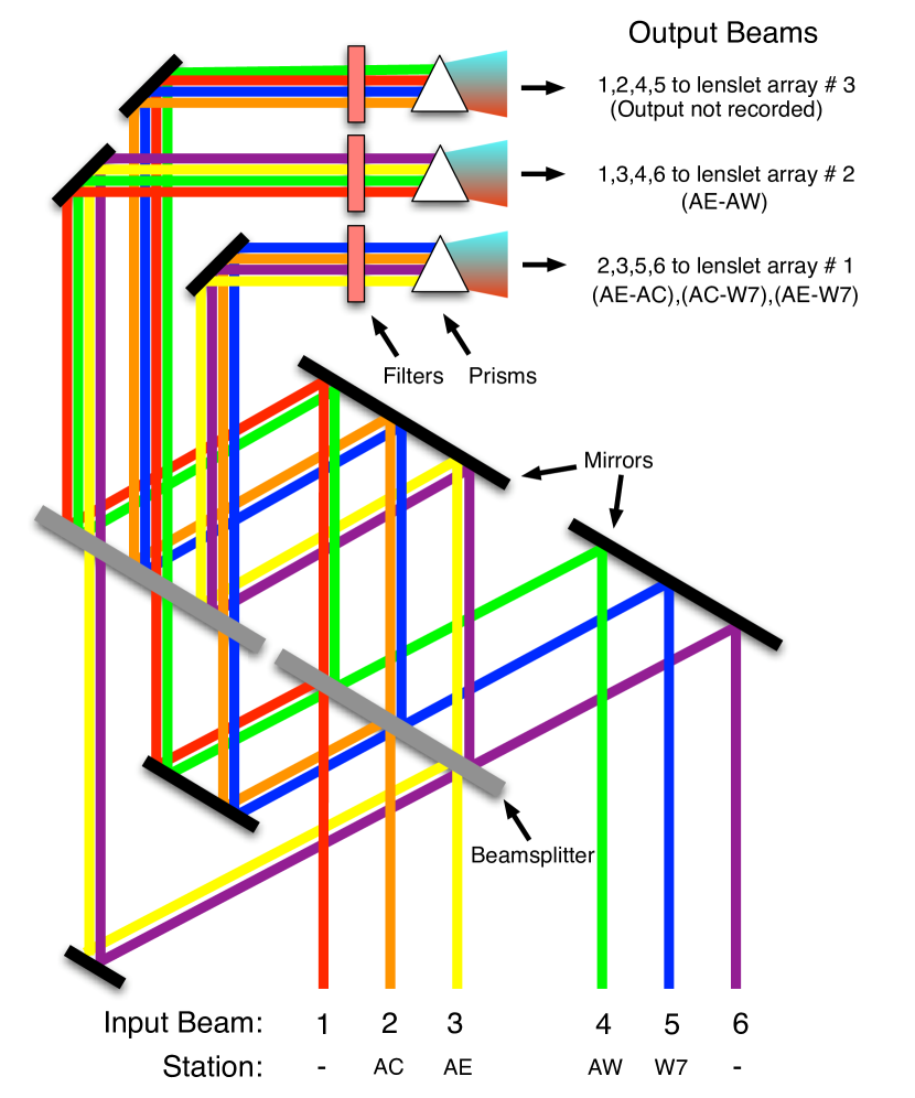
The instrument was designed to accept stellar light from up to 6 siderostats simultaneously, where each element sends a 12 cm light beam through vacuum pipes to the beam combiner lab. At the beam combiner, the light beams are split and recombined in such a way that the interference fringes between all siderostat pairs (for a total of 15 unique pairs) are constructed. Figure 2 illustrates the propagation of light for six input beams. The three output beams that are intercepted are dispersed by a set of three prisms onto individual lenslet arrays, which in turn are fiber-coupled to a cluster of photon-counting avalanche photodiodes. Each fiber corresponds to a single channel with spectral characteristics set by the position of the lenslet array and the physical width of a single lenslet along the dispersion direction.

The spectra of Be stars show many spectral lines in emission. For example, in the 510–880 nm region covered by our interferometric observations emission lines of elements such as H I, He I, O I, Si II, and Fe II can be detected. However, except for hydrogen lines all of the emission lines are very weak having equivalent widths (EW) of $\lesssim$ 0.1 nm, and therefore will be lost in the continuum signal present in each spectral channel (the widths of the spectral channels range from 10 to 26 nm). Even in the case of the hydrogen lines present in our spectral region of interest only the H$\alpha$ line has large enough EW to contribute a detectable interferometric signal in the H$\alpha$ containing channel. Therefore, for the purpose of the H$\alpha$ observations, the lenslet array is aligned such that the emission line is centered on a single channel that has a spectral width of 15 nm. Because the typical equivalent widths of H$\alpha$ emission lines in Be stars are usually not more than 4 nm (see for example Table 6 in Tycner et al., 2005), the contribution from the circumstellar region to the net signal is typically less than 25 %. For sources with very weak emission, the fractional contribution to the net signal can be much less than the magnitude of the random and systematic uncertainties, which are typically at the few percent level.

To increase the contrast between the interferometric signatures from the H$\alpha$-emitting circumstellar region and the central star, we have inserted a narrowband filter at each of the three outputs from the beam combiner (see Fig. 2). These filters have a high transmission ($\sim$90 %) in a 2.8 nm region centered on the H$\alpha$ line, which suppresses the nearby continuum emission, but does not significantly attenuate radiation outside a $\sim$100 nm region centered at the line. Because we need to detect the interferometric signal outside of the spectral channel containing the H$\alpha$ emission, for both calibration and fringe tracking purposes, the filter has high enough transmission in the 500–600 and 710–850 nm regions that the continuum channels are still usable. The transmission curve of the custom-made filter is shown in Figure 3 along with the superposed locations of the spectral channels that were used to record the fringe signals.

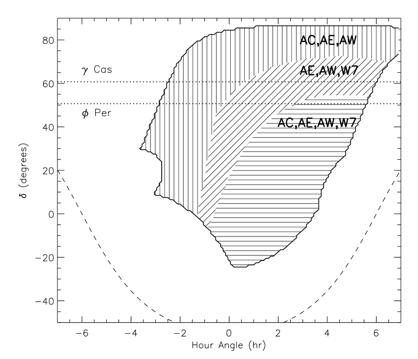
In the current instrumental setup the signals from up to 32 channels can be recorded simultaneously by the NPOI electronics. Because these channels are divided equally between two output beams from the beam combiner, data from one of the three output beams is currently not recorded (recall Fig. 2). This results in interferometric observations that do not sample all the baseline configurations that are possible with a given set of elements, as shown in Figure 1. Furthermore, because the long-delay lines are not implemented yet, the maximum path difference that can be introduced between a pair of siderostats (to compensate for the different distances between each station and the star) is currently 35 m and this results in restricted ranges of declination and hour angle over which a star can be observed at a given baseline. For example, Figure 4 shows the accessible sky coverage for three different configurations; in one case all four elements (AC, AW, AE, and W7) are used and in the other two configurations either the AC or the W7 station is excluded. Therefore, for $\gamma$ Cas the observations utilizing the AC–W7 baseline are not currently possible, whereas for $\phi$ Per, which is 10^∘ lower in the sky, such observations are possible. Of course, with the expected implementation of the long delay-lines, optical path difference compensation of up to $\sim$400 m will become possible and the accessible sky coverage will be significantly less restrictive.

3 Observations

3.1 Interferometry

The typical NPOI observing and data reduction procedures are described in Hummel et al. (2003). Here we provide a brief review of the process. During a 30 s observation fringe data are recorded every 2 ms. The squared visibility ($V^{2}$) estimators from the 2 ms data are averaged on 1 s intervals and the 1 s data points are processed using a suite of custom reduction software. Outlier points are flagged on the basis of the residuals of the delay, seeing indicators, photon rates, and squared visibilities. Finally, depending on how many 1 s data points have been flagged as bad, up to 30 points are averaged to produce a single squared visibility measure for each 30 s interval, also known as a “scan”. Typically, following a procedure similar to that used in obtaining the $V^{2}$ data, the closure phase and triple amplitude can also be obtained for each scan. However, because these quantities were not obtained for the data presented in this paper, we do not include them in our discussion.

The $V^{2}$ value for a single scan is obtained in the same way for both the target and the calibrator star, as well as for the incoherent scans (also known as the “off-the-fringe scans”). The typical observational sequence consists of a pair of coherent and incoherent scans on a target, followed by the same pair of scans on a calibrator. The procedure is repeated for as long as the scans of the target star are acquired. The incoherent scans are necessary to estimate the additive bias terms affecting the squared visibility measures (see Hummel et al., 2003, for more details). The bias term is a squared visibility measure that one obtains in the case of a completely incoherent signal, which for an ideal system should be exactly zero. Because the calibration procedure removes multiplicative effects, the subtraction of the additive bias term must be performed before calibration corrections are applied. We remove the bias terms from the squared visibilities of both the target and the calibrator stars following the method described in Wittkowski et al. (2001) and Hummel et al. (2003).

As we have discussed in § 2, $\gamma$ Cas could not be observed on the AC–W7 baseline because of its high declination that places the star outside the accessible sky coverage (defined by the limits imposed by the optical path compensation components). $\phi$ Per was not constrained by the same limitation having slightly lower declination. Because the two stars are separated in right ascension by less than 50 min it was more efficient to observe both stars in the same mode (i.e., using only 3 stations). The loss of one station for $\phi$ Per was compensated by the extended hour angle range over which it was possible to observe this star (recall Fig. 4). Another advantage of having only one baseline on each spectrograph is the elimination of multi-baseline cross-talk effects that may be present in the data (Schmitt et al., 2005). The disadvantage of having only two simultaneous baselines is that some interferometric observables such as closure phase and triple amplitude could not be obtained because they require at least three simultaneous baselines.

We observed $\gamma$ Cas and $\phi$ Per during November and December of 2004. Although we lost many nights due to poor weather, we still managed to obtain $\sim$100 scans for each star with almost all the scans providing data on two baselines. Table 1 shows a log of the observations. On 2004 Dec 8 the vacuum pipes between the 6th and 7th station on each of the three arms were disconnected (see Fig. 1 for the layout of the imaging array) in order to install safety vacuum valves. This resulted in the W7 station being unavailable for observations starting 2004 Dec 10, and therefore, only observations utilizing the AE, AC and AW stations were recorded for the rest of the observing run. On 2004 Dec 2 we temporarily removed the narrowband filters from the outputs of the beam combiner to obtain observations without the use of the filters, but with the same instrumental configuration.

For the purpose of the analysis presented in this paper, we are only interested in the squared visibilities from the spectral channels that contain the H$\alpha$ emission line. However, before these $V^{2}$ values can be extracted from the observational data set, we need to calibrate these quantities. We follow the calibration procedure outlined in Tycner et al. (2003), which we only summarize here. The calibration procedure uses the continuum channels at a given scan and baseline to estimate a correction function that has a quadratic dependence in $\lambda^{-1}$, which is then applied to the squared visibility measure in the spectral channel that contains the H$\alpha$ emission line. Because the correction function is a slowly varying function across channels, it cannot account for any high order channel-to-channel variations. Therefore, in the current analysis we estimated the $V^{2}$ amplitudes of the high order variations across the spectral channels using the residuals that could not be removed with the quadratic polynomials from the scans of the calibrator stars. The calibrators used for $\gamma$ Cas and $\phi$ Per were $\epsilon$ Cas (=HR 542) and $\zeta$ Cas (=HR 153), respectively. Both calibrators are B-type stars and were verified by spectroscopic observations to have H$\alpha$ in absorption. After confirming that the channel-to-channel variations established based on observations of the calibrators are stable on time scales longer than one night, we calculated nightly averages that were then divided out of the scans of the target stars.

After applying the bias and the calibration corrections to all scans, we extract the squared visibilities for the H$\alpha$ channel forming two large data sets, one for $\gamma$ Cas (with 169 data points) and the other for $\phi$ Per (with 186 data points). The observations obtained on 2004 Dec 2, when the narrowband filters were not used, are treated as separate data sets. Figures 5 and 6 show the resulting ($u,v$)-plane coverage at the AC–AE, AE–AW, and AE–W7 baselines in the H$\alpha$ channel for $\gamma$ Cas and $\phi$ Per, respectively. The corresponding $V^{2}$ data for the two stars are shown in Figures 7 and 8 for observations obtained with the narrowband filter, whereas the $V^{2}$ observations obtained without the filters are shown in Figures 9 and 10.

3.2 Spectroscopy

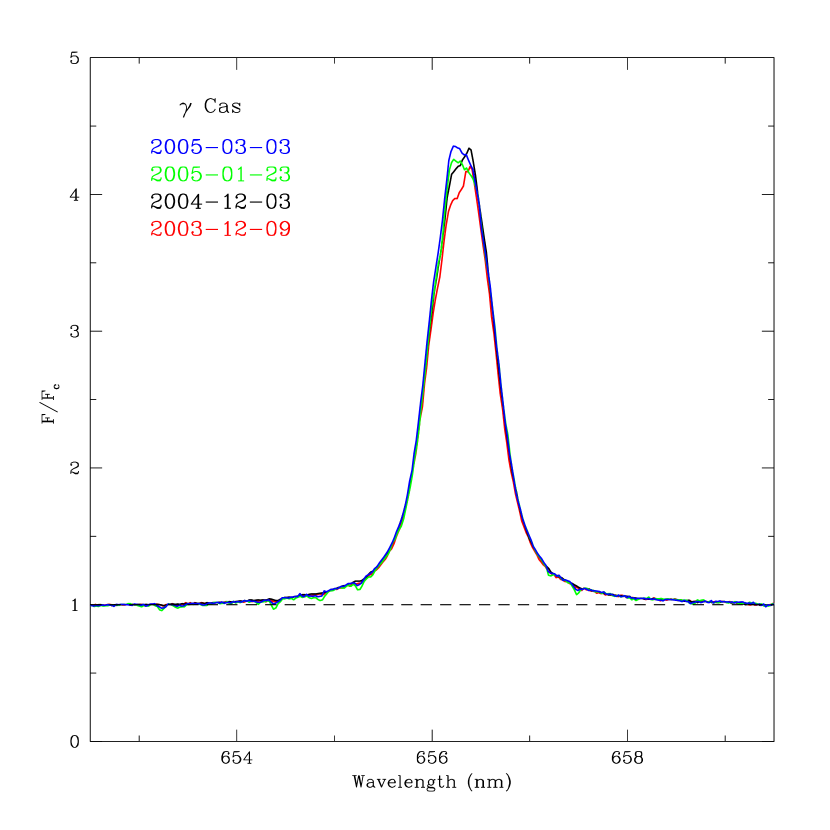
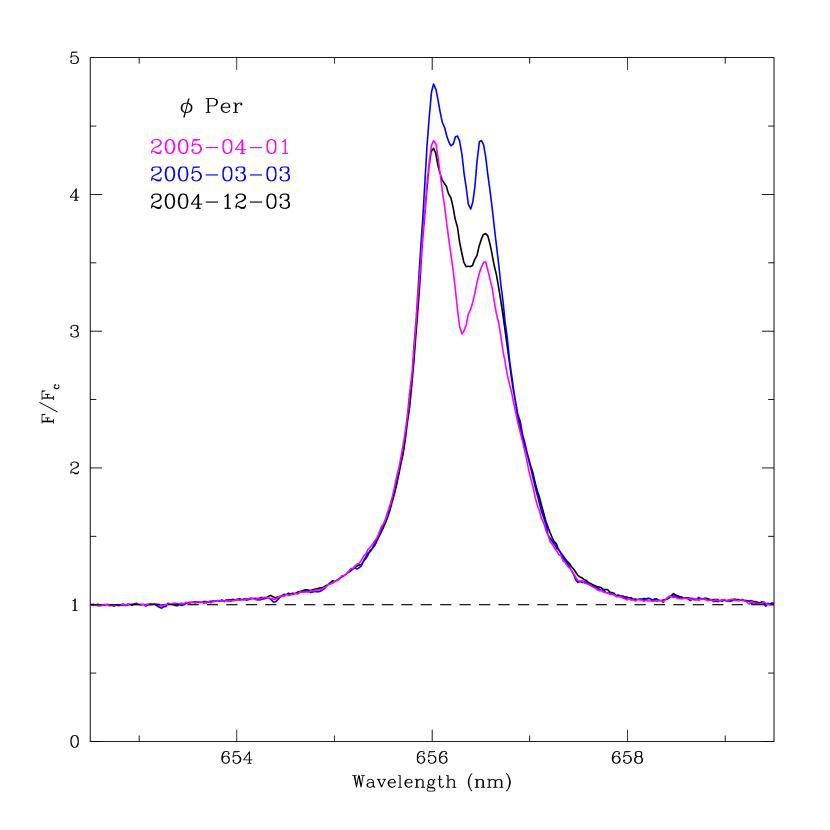
The interferometric observations obtained with the NPOI do not contain enough spectral information to help us establish the properties of the H$\alpha$ emission line. Therefore, we observed $\gamma$ Cas and $\phi$ Per using a fiber-fed echelle spectrograph (also known as the Solar-Stellar Spectrograph; SSS), which is located at the Lowell Observatory’s John S. Hall 1.1 m telescope. The SSS instrument produces spectra in the H$\alpha$ region with the resolving power of $\sim$10,000 and a signal-to-noise ratio (SNR) of few hundred in the H$\alpha$ region. The SSS observations were reduced using standard reduction routines written in IDL (Hall et al., 1994), and the resulting H$\alpha$ profiles of $\gamma$ Cas and $\phi$ Per are shown in Figures 11 and 12, respectively.

The H$\alpha$ emission of $\gamma$ Cas is known to be stable on time scales greater than $1$ yr and our spectra confirm this. The EWs of the four H$\alpha$ profiles shown in Figure 11 range from $-3.0$ to $-3.2$ nm. Because the largest uncertainty associated with these values is the precision of continuum normalization, which we estimate at 3%, for the purpose of our study we use an EW of $-3.1\pm 0.1$ nm for the H$\alpha$ emission of $\gamma$ Cas.

As we will discuss in § 5.3, $\phi$ Per is a Be+sdO spectroscopic binary with a period of 127 d and is known to show H$\alpha$ variability. The observed variability is attributed in part to the radiative effects of the hot secondary on the circumstellar region associated with the primary. Although our temporal coverage is limited, we confirm the presence of H$\alpha$ emission variability in $\phi$ Per. The equivalent widths of the three profiles shown in Figure 12 are $-3.8$, $-4.2$, and $-3.6$ nm, which were obtained on 2004 Dec 3, 2005 Mar 3, and 2005 Apr 1, respectively. However, because the relative shape of the H$\alpha$ profile does not appear to change significantly, we conclude that combining all of the interferometric observations from our observing run should not result in any significant errors (we will return to this point in § 4.2). For this reason we adopt an H$\alpha$ EW for $\phi$ Per of $-3.9\pm 0.3$ nm, where the larger uncertainty should account for the intrinsic variability during our interferometric run.

4 The Analysis

4.1 Models

The squared visibilities from the spectral channels containing the H$\alpha$ emission contain two signatures, one due to the central star and the other due to the circumstellar region. Therefore, these data must be modeled with a two component model of the form

$$V^{2}_{\rm model}=\left[c_{p}V_{p}+(1-c_{p})V_{\rm env}\right]^{2},$$ (1)

where $V_{p}$ and $V_{\rm env}$ are the visibility functions representing the photosphere of the central star and the circumstellar envelope, respectively, and $c_{p}$ is the fractional contribution from the stellar photosphere to the total flux in the H$\alpha$ channel. Generally, both $V_{p}$ and $V_{\rm env}$ can be complex functions, but because the models we consider in this analysis are all point-symmetric, as well as concentric, the functions are real and can be treated as visibility amplitudes.

To decrease the number of free parameters in our models we treat the angular diameter of the central star as a known quantity. This is also supported by the fact that the central stars are not significantly resolved even at our longest baseline. Furthermore, as we discussed in Tycner et al. (2004), our best-fit models describing the H$\alpha$-emitting regions are not very sensitive to the assumed diameter of the central star (changing the diameter by a factor of 2 results in $\sim$ 1 % change in the best-fit disk parameters). For the same reason we can also ignore any effects related to the rapid rotation for which Be stars are well known for, because the geometrical distortion and gravity darkening near the stellar equator will only weakly affect our best-fit disk parameters.

The most widely used approach for predicting a stellar angular diameter is to use empirically established relationships between the stellar color index and the surface brightness, which in turn is related to the angular size (Barnes et al., 1978; van Belle, 1999). Another approach would be to use tabulations of linear stellar diameters as a function of spectral class (Underhill et al., 1979). However, because there is an intrinsic scatter in stellar diameters at each spectral class, and the distance to the source needs to be known to convert the linear diameter to the angular size needed for interferometry, this is not the preferred approach. Therefore, for $\gamma$ Cas and $\phi$ Per we adopt the same stellar angular diameters as were used by Quirrenbach et al. (1997), which were derived using the photometric relations of Barnes et al. (1978). The angular diameters we adopt for $\gamma$ Cas and $\phi$ Per are 0.56 and 0.39 mas, respectively.

We model the stellar photosphere of each star with a circularly symmetric uniform disk brightness distribution. This ensures that the central star is modeled in exactly the same way, at the continuum channels during the calibration procedure (see Tycner et al., 2003, for more details) and at the H$\alpha$ channel via equation (1). Therefore, we represent the visibility function of the photospheric component of an angular diameter $a$ with

$$V_{p}(u,v)=2\frac{J_{1}(\pi a\sqrt{u^{2}+v^{2}})}{\pi a\sqrt{u^{2}+v^{2}}},$$ (2)

where $J_{1}$ is a first-order Bessel function and $u$ and $v$ are the spatial frequencies, which are given by the east-west and south-north components of the projected baseline on the plane of the sky divided by wavelength (see §4.1 in Thompson et al., 2001, for the definition of $u$-$v$ plane).

Our interferometric observations were obtained at high spatial frequencies (i.e., at high spatial resolution), and therefore, we can compare different models of brightness distribution. Previously published work on disk models of Be stars has demonstrated that the thermal structure of the circumstellar disks can be quite complex (Millar & Marlborough, 1998; Millar et al., 2000; Carciofi & Bjorkman, 2006). However, for this first investigation with this new observational technique we choose to model our data with three simple models, uniform disk (UD), uniform ring (UR), and a Gaussian distribution (GD). The visibility amplitudes for all three models can be written as

$$V_{\rm env}=\left\{\begin{array}[]{c@{\quad:\quad}l}2J_{1}(\pi\theta_{\rm UD}s)/\pi\theta_{\rm UD}s&{\rm UD}\\ 2(1-\epsilon^{2})^{-1}[J_{1}(\pi\theta_{\rm UR}s)/\pi\theta_{\rm UR}s-\epsilon^{2}J_{1}(\pi\epsilon\theta_{\rm UR}s)/\pi\epsilon\theta_{\rm UR}s]&{\rm UR}\\ \exp[-(\pi\theta_{\rm GD}s)^{2}/4\ln 2]&{\rm GD}\end{array}\right.,$$ (3)

where $\theta_{\rm UD}$, $\theta_{\rm UR}$ correspond to the angular diameters of the UD and UR models, respectively, and $\theta_{\rm GD}$ corresponds to the full-width at half-maximum (FWHM) of the Gaussian model. Because we allow all three models to have elliptical distribution on the sky, all of the above diameters describe the dimensions along the major axis. The other variables in equation (3) are, $\epsilon$ that describes the inner diameter of the ring model along the major axis (in units of $\theta_{\rm UR}$), and $s$ that is given by

$$s=\sqrt{r^{2}(u\cos\phi-v\sin\phi)^{2}+(u\sin\phi+v\cos\phi)^{2}},$$ (4)

where $r$ is the axial ratio and $\phi$ is the position angle (PA; measured east from north) of the major axis (when $0\leq r<1$). For circularly symmetric structures ($r=1$), equation (4) reduces to a simple expression for a radial spatial frequency in the $(u,v)$-plane that is given by $(u^{2}+v^{2})^{1/2}$.

4.2 Model Fitting

To obtain a best-fit for each of the three models, we used a nonlinear least-squares IDL procedure based on the Levenberg-Marquardt method (Press et al., 1992). Each model is represented by equation (1), with the appropriate expression for the envelope component from equation (3), and a fixed visibility function for the photospheric component (eq. [2] with a fixed stellar diameter $a$). Therefore, the UD and GD models have four free parameters, $c_{p}$, $\theta$, $r$, and $\phi$, whereas the UR model has $\epsilon$ as an extra parameter. Table 2 lists the best-fit values for the parameters for all three models along with the reduced $\chi^{2}$ values. By inspecting the reduced $\chi^{2}$ values in Table 2 for the three $\gamma$ Cas models, it is evident that the UD and UR models cannot represent the observations obtained at all three baselines. Therefore, we have also fitted models to observations of $\gamma$ Cas from the shortest two baselines only, where all three models yield similar quality fits (these models are also listed in Table 2). To check for any possible variations in the models that could be attributed to the temporal variability of our sources (especially in the case of $\phi$ Per), we fitted models to various subsets of our large data set. Although typically the uncertainties of the best-fit parameters are larger for models fitted to smaller data sets, all results were consistent with our solutions based on all observations.

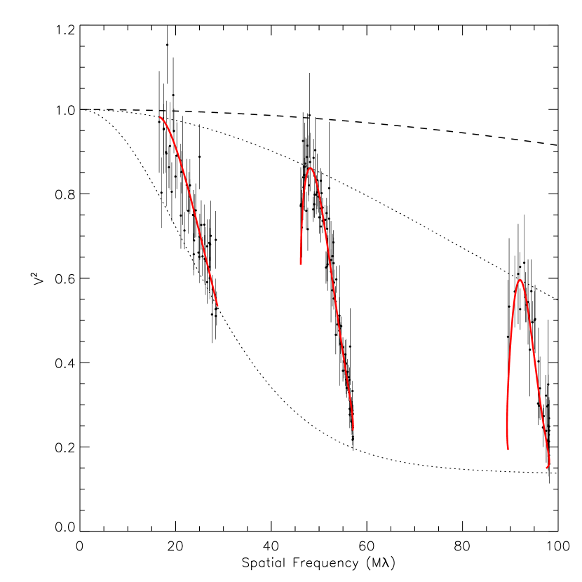
To illustrate why the UD and UR models fail to represent the observations of $\gamma$ Cas obtained at all three baselines, in Figure 13 we plot the best-fit UD, UR, and GD models, which were only fitted to data from the shortest two baselines. Each baseline provides data over a different spatial frequency range (because of different physical lengths) and these ranges are marked with thick solid lines in Figure 13. A small fraction of each range corresponds to an instant at which the projected baseline on the sky was oriented along the major axis for which these model curves were evaluated. The model curves demonstrate the inherent degeneracy present between the three models at low spatial frequencies (i.e., at low spatial resolutions the three models look the same). However, the longest baseline provides data at high enough spatial frequencies so that the degeneracy between the three models is eliminated (see also Fig. 7). We conclude that the UD and UR models are inconsistent with the data obtained at the longest baseline (largest spatial frequencies), whereas the GD models fit the observations at all baselines.

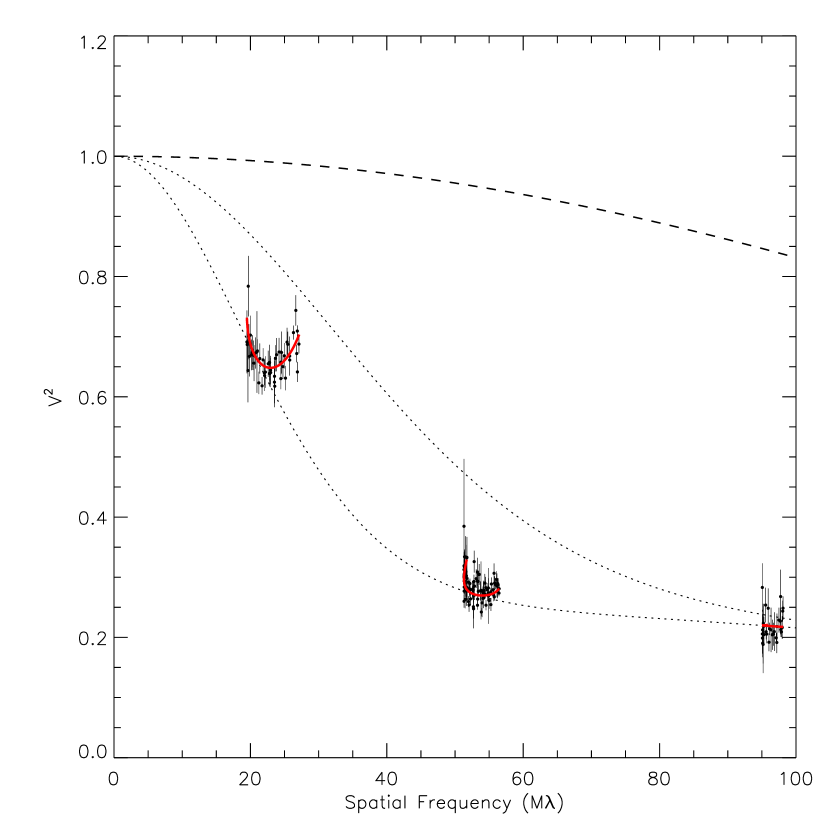
The observations of $\phi$ Per are more challenging because the angular size of its circumstellar region is smaller than for $\gamma$ Cas, as well as the projected baselines on the plane of the sky are not oriented along its major axis. This results in interferometric observations that do not resolve the region sufficiently well to break the degeneracy between the different models. This is also the reason all three models for $\phi$ Per listed in Table 2 yield the same $\chi^{2}_{\nu}$ values. Figure 14 demonstrates the differences between the model curves based on the three best-fit models evaluated at three different projections. The three projections were chosen to correspond to the minor axis (that is 27% of the major axis), along a direction where the extent is 50% of the major axis, and along the major axis. Because we do not have observations that resolve the major axis (recall Fig. 8), the spatial frequency ranges over which we have data are marked only on the curves that correspond to the minor axis and 50% of the major (marked with thick solid lines in Fig. 14). Based on Figure 14 we conclude that in order to break the degeneracy between the models, either observations at higher spatial frequencies, or along the major axis, are required (as demonstrated in the case of $\gamma$ Cas).

4.3 Gaussian Distribution

For $\phi$ Per we cannot exclude the UD and UR models in favor of the GD model based on interferometric data alone, however, we can demonstrate that the GD model is the preferred solution. This is because the three models that fit the $\phi$ Per data equally well, have different best-fit values for the $c_{p}$ parameter, which can be constrained by spectroscopy. For example, if the EW of the continuum flux from the star in the H$\alpha$ channel is $F_{\star}$ (which has units of length) and the EW of the net H$\alpha$ emission is $E_{{\rm H}\alpha}$, then the fractional photospheric contribution in the absence of a narrowband filter ($c_{p}^{\star}$) can be expressed as

$$c_{p}^{\star}=\frac{F_{\star}}{F_{\star}+E_{{\rm H}\alpha}}.$$ (5)

With the narrowband filter $F_{\star}$ gets reduced to $tF_{\star}$, where $t$ is the fractional transmission in the H$\alpha$ channel. The H$\alpha$ emission gets reduced by the filter as well, but because the H$\alpha$ emission lines have FWHM $\lesssim$ 1nm, which is less than the width of 2.8 nm of the narrowband region, we can approximate the transmission at the H$\alpha$ line ($\eta$) by the peak transmission of 92 % of the narrowband region (recall Fig. 3). Therefore, the $c_{p}$ parameter for the case including the filter can be written as

$$c_{p}=\frac{tF_{\star}}{tF_{\star}+\eta E_{{\rm H}\alpha}}.$$ (6)

Taking the ratio of equations (5) and (6) allows us to obtain an expression for $t$ of the form

$$t=\eta\frac{1/c_{p}^{\star}-1}{1/c_{p}-1},$$ (7)

which does not depend on $F_{\star}$ or $E_{{\rm H}\alpha}$.

Equation (7) requires the photospheric contributions $c_{p}$ and $c_{p}^{\star}$ to be known. For $c_{p}$ we use the values listed in Table 2 obtained for the GD model fits to observations with the narrowband filters. To obtain the corresponding values for $c_{p}^{\star}$, we fit GD models to observations obtained without the filters (i.e., the observations obtained on 2004 Dec 2). The squared visibilities for the best-fit models to the 2004 Dec 2 data are shown in Figures 9 and 10, for $\gamma$ Cas and $\phi$ Per, respectively. In both cases the best-fit GD model parameters (except for $c_{p}$) agree with the parameters listed in Table 2, even for $\gamma$ Cas where we did not have enough points to constrain an elliptical model. These fits yield $c_{p}^{\star}$ values of 0.85 and 0.78 for $\gamma$ Cas and $\phi$ Per, respectively. Using equation (7) with the appropriate values for $\gamma$ Cas and $\phi$ Per we obtain the same estimate for $t$ of $0.17\pm 0.01$. It is interesting to note that this 17 % transmission is fully consistent with the detected drop in photon counts in the H$\alpha$ channel when the narrowband filters are introduced for observations of calibrator stars (which do not have H$\alpha$ in emission).

Because our estimate for $t$ does not dependent on $F_{\star}$ or $E_{{\rm H}\alpha}$, we can use equation (6) to obtain a value for $c_{p}$ based on spectroscopic observations. We approximate $F_{\star}$ with the spectral width of the H$\alpha$ channel (which has been measured to be $15\pm 1$ nm). To obtain the EW of the net H$\alpha$ emission for $\phi$ Per, we use the H$\alpha$ EW from § 3.2 and we add a small contribution (0.37 nm) due to the absorption line that has been filled in (using the same procedure as outlined in § 4.2 of Tycner et al., 2005). The net H$\alpha$ emission of $4.27\pm 0.30$ nm for $\phi$ Per results in $c_{p}$ of $0.39\pm 0.03$. This estimate is significantly lower than the values listed in Table 2 for the UD and UR models, which have best-fit $c_{p}$ values of 0.52 and 0.62, respectively, but it is fully consistent with the $0.39\pm 0.02$ value obtained for the GD model. We interpret this as an indication that the brightness distribution of the circumstellar disk of $\phi$ Per is best represented by a GD model. It is interesting to note, if we follow the same reasoning for $\gamma$ Cas data from the shortest two baselines (where the degeneracy between the three models also exists) we arrive at the same conclusion that the GD model is the preferred solution. For $\gamma$ Cas, based on its H$\alpha$ EW of $-3.1\pm 0.1$ nm and an estimated component accounting for the absorption line of 0.26 nm, we estimate that $c_{p}=0.45\pm 0.03$, which again is closest to the value obtained for the GD model.

We conclude that out of the three models we have considered in our analysis the GD model is the only model that fits $\gamma$ Cas observations and is the preferred model for $\phi$ Per based on spectroscopic constraints. Therefore, in Table 3 we list our final best-fit parameters describing the circumstellar regions of $\gamma$ Cas and $\phi$ Per based on the GD model fits. The model squared visibilities calculated based on these models are shown with red solid lines in Figures 7 and 8 for $\gamma$ Cas and $\phi$ Per, respectively.

5 Discussion

5.1 Circumstellar Region

Because the number of published parameters describing the circumstellar regions of $\gamma$ Cas and $\phi$ Per is still very small, it is worthwhile to compare our results to those published in the literature. Both, Quirrenbach et al. (1997) and Tycner et al. (2003) fitted a GD model to their observations and therefore their model values can be compared directly with those listed in Table 3.

Using observational data from the Mark III interferometer Quirrenbach et al. (1997) obtained best-fit model parameters for $\gamma$ Cas of $\theta=3.47\pm 0.02$ mas, $r=0.70\pm 0.02$, and PA of 19$\pm 2^{\circ}$. Tycner et al. (2003) reported results based on older NPOI observations (with a maximum baseline of 37.5 m), which had $\theta=3.67\pm 0.09$ mas, $r=0.79\pm 0.03$, and PA of 32$\pm 5^{\circ}$. Our new determination of the angular size of the major axis of $3.59\pm 0.04$, fully confirms the previous estimates. The apparent axial ratio of $0.58\pm 0.03$ that we find for $\gamma$ Cas is smaller than the published values and this might be related to the fact that our interferometric observations cover much larger range of baseline projection angles on the plane of the sky (recall Fig. 5). Our best-fit value for the PA of $31\fdg 2\pm 1\fdg 2$ agrees with our previous estimate (Tycner et al., 2003), but differs from the PA reported by Quirrenbach et al. (1997) whose value was at right angle to the polarization vector they obtained from polarimetry. Possible sources for this discrepancy could be the intrinsic variability of the polarization of the source (see for example Table 6 in Quirrenbach et al., 1997), the residual effects associated with the removal of the interstellar polarization, or the effects of non-axisymmetric scattering surface (i.e., only for axisymmetric sources can one expect the polarization vector to be exactly perpendicular to the plane of the disk).

For $\phi$ Per, Quirrenbach et al. (1997) obtained model values of $\theta=2.67\pm 0.20$, $r=0.46\pm 0.04$, and PA of $-62\pm 5^{\circ}$, but they point out that the value for $r$ might be an upper limit because their baselines were not long enough to resolve the minor axis. Indeed, our results based on observations that utilize baselines that are more than twice as long than those used in their study yield a best-fit value of $0.27\pm 0.01$ for the axial ratio. However, the angular size of the major axis of $2.89\pm 0.09$ and PA of $-61\fdg 5\pm 0\fdg 6$ that we obtain in this study fully agree with their values. Since $\phi$ Per was not observed by any other interferometer than Mark III, our results represent the first confirmation of the values reported by Quirrenbach et al. (1997).

5.2 Inclination and Disk Opening Angles

Our interferometric observations of the spatially resolved circumstellar regions, which show an apparent ellipticity, can be used to estimate the inclination and disk-opening angles. For example, if we assume that the circumstellar disk is circularly symmetric, we can obtain a lower limit on the inclination angle ($i$) using the observed axial ratio ($r$) using

$$i\gtrsim\cos^{-1}r.$$ (8)

The minimum value corresponds to a geometrically thin disk, where the entire signature of the apparent ellipticity is interpreted as a projection effect in this case. Similarly, if we assume that the geometry of the circumstellar region can be represented with a simple equatorial disk model with a half-opening angle $H_{\theta}$ and radius $R_{\rm disk}$ (see for example Fig. 2 in Waters et al., 1987), we can then obtain an upper limit on $H_{\theta}$ using

$$H_{\theta}\lesssim\sin^{-1}(r/2),$$ (9)

where the maximum value corresponds to a system viewed edge-on.

In Table 3 we list the estimated limits on the inclination and half-opening angles for both $\gamma$ Cas and $\phi$ Per based on their best-fit values of $r$ obtained from the elliptical Gaussian models. Interestingly, for $\phi$ Per the lower limit of $\approx$ 74^∘ for $i$ is consistent with the 80^∘ to $88^{\circ}$ range originally proposed by Poeckert (1981). Although Poeckert (1981) did not describe the circumstellar region in terms of an opening angle, the disk thickness of 1.3–2.7 $R_{\star}$ and the disk radius of 7.7 $R_{\star}$ can be translated to a half-opening angle between 5 and 10^∘, which again is consistent with our upper limit of $\approx 8^{\circ}$.

It is instructive to compare the upper limits we obtain for $H_{\theta}$ of $\gamma$ Cas and $\phi$ Per to the value of 15^∘ adopted by Waters et al. (1987) in their study of almost 60 Be stars based on far-IR IRAS observations. Waters et al. (1987) estimated a number of different Be stellar characteristics, such as the mass loss rate and the disk density, which had a dependence on $H_{\theta}$. Although the authors assumed an error of a factor of 1.5 in $\sin H_{\theta}$, our upper limit for the disk half-opening angle for $\phi$ Per is half their adopted value. In the case of $\phi$ Per, the mass loss rate derived by Waters et al. (1987) will be overestimated by at least a factor of two, or more if the source is not viewed edge-on. Our upper limit on the half-opening angle of 17^∘ for $\gamma$ Cas is consistent with the value adopted by Waters et al. (1987). However, based on the line profile classification scheme established by Hanuschik et al. (1996) we can conclude that $\gamma$ Cas is not viewed edge-on and therefore its half-opening angle is most likely less than 17^∘. In the case of the Be star $\zeta$ Tau, for which the apparent ellipticity of the circumstellar region has also been detected (Quirrenbach et al., 1997; Tycner et al., 2004), one can conclude that $H_{\theta}\lesssim 9^{\circ}$. It is possible that other Be stars also have small disk opening angles. To further test the generality of this hypothesis, future interferometric observations should concentrate on systems that are thought to be viewed at large inclination angles (for example using H$\alpha$ profile classification of Hanuschik et al., 1996).

We can also compare our interferometrically determined opening angles with those predicted by Stee (2003) who has calculated the disk opening angles for a number of Be stars based on the flux in the Brackett continuum near 2.2 $\mu$m using the SIMECA code (Stee & de Araujo, 1994; Stee et al., 1995). The main characteristic of the SIMECA model is that for a fixed disk density at the stellar photosphere, the opening angle is directly proportional to the continuum flux, so that a large flux in the $K$-band corresponds to a large opening angle. For example, Stee (2003) obtained a value of 14^∘ for the full-opening angle of the disk of $\phi$ Per, which agrees with our upper value of 16^∘. However, our upper limit for the full-opening angle for $\gamma$ Cas is 34^∘, which is significantly less than the 54^∘ obtained by Stee (2003) for this star. This discrepancy may be due to the fact that Stee (2003) might have used apparent and not absolute magnitudes to derive the disk-opening angles, in which case the values reported in that study should be reevaluated.

5.3 Disk Truncation

Tycner et al. (2004) showed that the H$\alpha$-emitting region of the binary Be star $\zeta$ Tau was well within the estimated Roche lobe of the primary, which suggests that the disk is truncated. Another example of a possible disk truncation was presented by Chesneau et al. (2005) for $\alpha$ Ara, where the VLTI operating in the $N$ band did not resolve any structure and therefore allowed the authors to put an upper limit on the extent of the circumstellar region. Because this limit was smaller than the expected spatial extent based on the models that were fitted to the Balmer emission lines, the authors suggest that disk truncation by an unseen companion might be occurring.

Evidence is accumulating which suggests that $\gamma$ Cas is a member of a binary system. Harmanec et al. (2000) published the first orbital radial velocity curve for $\gamma$ Cas based on observations collected in the 628–672 nm range from 1993 to 2000. Their analysis suggests that this star is the primary component of a spectroscopic binary with a period of $\approx 204$ days and an eccentricity of 0.26. This result was confirmed by Miroshnichenko et al. (2002) using high-resolution spectroscopic observations of the H$\alpha$ line obtained over a similar time period. They report a periodic change of 205 days in this line, which they also attribute to the binary system. Although Harmanec et al. (2000) concludes that the secondary could be either a hot compact object or a low luminosity late-type star, they estimate that the separation between the components at periastron could be between 250 and 300 $R_{\sun}$. The distance to $\gamma$ Cas is $188\pm 20$ pc based on the Hipparcos satellite measurements (Perryman et al., 1997), which places the separation between the components at 6.2–7.4 mas. Our best-fit value for the FWHM of the major axis is $3.59\pm 0.04$ and therefore the circumstellar disk is well within the orbit established by Harmanec et al. (2000). However, because the binary parameters of $\gamma$ Cas are not well established this comparison is tentative.

The binary nature of $\phi$ Per is much better established since it was recognized as a binary in the early 1900’s (Cannon, 1910; Ludendorff, 1911). Poeckert (1981) documents the development in the understanding of $\phi$ Per’s binary nature over the succeeding decades, and suggests that a subdwarf O star is the secondary. Gies et al. (1998) detected the secondary in ultraviolet spectra obtained with the Hubble Space Telescope and confirmed Poeckert’s prediction. $\phi$ Per is now part of a group of four candidate Be$+$sdO binaries, the others being HR 2142 (Waters et al., 1991), 59 Cyg (Maintz, 2003), and FY CMa (Rivinius et al., 2004). Be$+$sdO binaries may result from a spin-up of the B star as a result of mass transfer from the progenitor of the evolved subdwarf companion.

Estimates of the orbital parameters of $\phi$ Per are available in Božić et al. (1995) and Gies et al. (1998). The semi-major axes of these two orbital solutions range from approximately 230 to 310 R_⊙. Using the Hipparcos distance of 220${}^{+43}_{-31}$ pc for $\phi$ Per (Perryman et al., 1997) we expect an angular separation of 4.9–6.6 mas between the components of $\phi$ Per. As we would expect, this separation is larger than the angular radius of any of the models of $\phi$ Per listed in Table 2. The radial extent of the Gaussian model can be approximated with the FWHM measure of 3.12$\pm$0.08 mas (148$\pm$30 $R_{\sun}$) we obtain for $\phi$ Per (i.e., we are assuming that the radial extent is twice the half-width of the Gaussian). This disk radius is very close to the 178–204 $R_{\sun}$ Roche radius of the primary obtained by Božić et al. (1995). This is most likely another example of a H$\alpha$-emitting region that is close in size to the actual extent of the circumstellar region, and this suggests that disk truncation is occurring in this system.

We should note that in the case of $\phi$ Per the presence of a truncated disk has been predicted. Waters (1986) used the IRAS observations of $\phi$ Per at 12, 25, and 60 $\mu$m to measure the IR excess and constrained the density distribution of $\rho(R)=\rho_{o}(r/R_{\star})^{-n}$ with $n=3.1$ for the disk model. Because he obtained a value of $n=2.4$ for two other Be stars, $\delta$ Cen and $\chi$ Oph, which also happens to correspond to a velocity law that has more gradual increase with distance (something that is predicted based on the H$\alpha$ spectroscopy), he argued that a density distribution with $n=2.4$ might be more appropriate for $\phi$ Per, which could be only satisfied if the disk model was truncated at $\sim 6.5R_{\star}$ (or $\sim$46 $R_{\sun}$). The apparent discrepancy between our values for the size of the truncated disk might be related to the different wavelength regimes of our studies, as well as to the assumption made by Waters (1986) that the system is viewed pole-on, whereas $i$ might be very close to 90^∘.

Poeckert (1981) also predicted a second H$\alpha$-emitting disk associated with the secondary component. Although our $V^{2}$ data in the H$\alpha$ channel does not have a very high SNR, we do not detect any deviations from the elliptical Gaussian model that would suggest a binary signature in the H$\alpha$ signal. Therefore, we are forced to conclude that if the secondary star does possess a H$\alpha$ emitting disk it does not contribute significantly to the net H$\alpha$ emission line. This is also consistent with the secondary’s disk radius of 6–8 $R_{\sun}$ estimated by Božić et al. (1995) based on the peak separation of the He II emission line. Assuming that the H$\alpha$ emission is proportional to the area of the disk, as demonstrated by Tycner et al. (2005), we conclude that the H$\alpha$ emission from the disk of the secondary will contribute less than $\sim$1% to the total H$\alpha$ flux.

The direct detection of the secondary with the NPOI is unlikely as Gies et al. (1998) report a brightness ratio of 0.15 (or $\Delta$m of 2) at 164.7 nm. The NPOI operates over a bandwidth of 550–850 nm and at these wavelengths the magnitude difference between the two components is likely to be much larger than 2. A search for a binary signature (a sinusoidal variation) across the continuum channels in both $\gamma$ Cas and $\phi$ Per yielded null results. On the other hand, a binary signature with a small $V^{2}$ amplitude (less than $\sim$3 %) could not be ruled out. In fact, it might be possible to detect the signature of binarity in both stars at longer wavelengths since $\gamma$ Cas may be associated with a cool companion, and $\phi$ Per might contain large contributions from the circumstellar disks of both components due to the free-free and free-bound emission.

6 Conclusions

We have successfully demonstrated the use of a narrowband filter in the NPOI to increase the contrast between the H$\alpha$-emitting material and the central star. Our observations of two Be stars, $\gamma$ Cas and $\phi$ Per, and our subsequent analysis have yielded the following results:

1. We have demonstrated that the uniform disk or ring-like models are inconsistent with the observations of the circumstellar region of $\gamma$ Cas, whereas a Gaussian model is fully consistent with the data. However, since the thermal structure of the circumstellar disks of Be stars can be quite complex, as suggested by recent models (Millar & Marlborough, 1998; Carciofi & Bjorkman, 2006), it might turn out that a more complicated brightness distributions may be required to fully describe these regions.

2. The circumstellar disk of $\gamma$ Cas appears to be consistent with the orbital parameters published in the literature. However, higher precision binary solutions are required to test for the possible disk truncation by the secondary.

3. Based on interferometric and spectroscopic data we have shown that the brightness distribution of the H$\alpha$-emitting circumstellar region of $\phi$ Per is best represented by a Gaussian distribution.

4. Our analysis supports the earlier prediction by Waters (1986) that the disk of $\phi$ Per is truncated due to the presence of an orbiting companion. However, the disk size we report is different than the value determined by Waters (1986). This discrepancy is likely due to different wavelength regimes used in each study and/or due to the low inclination angle assumed by Waters (1986) for this star, whereas we obtain $i\gtrsim 74^{\circ}$.

A natural extension of the analysis presented in this study is the direct comparison of interferometric data with theoretically predicted interferometric observables, such as synthetic squared visibilities. Future observations and modeling are planned that combine narrowband interferometry with spectroscopy for several other Be stars, especially those that possess weak H$\alpha$ emission. The goal of this work is to place greater constraints on the spatial extent and physical properties of the circumstellar material. These constraints will allow various dynamical models to be tested with greater certainty.

The Navy Prototype Optical Interferometer is a joint project of the Naval Research Laboratory and the US Naval Observatory, in cooperation with Lowell Observatory, and is funded by the Office of Naval Research and the Oceanographer of the Navy. We would like to thank Susan Strosahl and Dale Theiling for their contribution to the NPOI project through nightly observing, and Brit O’Neill for the assistance with the H$\alpha$ filter setup. We would also like to acknowledge the support of Jeff Munn for providing the observation planning software, and Christian Hummel for the OYSTER reduction software. We also thank the anonymous referee for the useful comments on how to improve this manuscript. C.T. thanks Lowell Observatory for the generous time allocation on the John S. Hall 1.1 m telescope and thanks Wes Lockwood and Jeffrey Hall for supporting the Be star project on the Solar-Stellar Spectrograph. C.T. acknowledges that this work was performed under a contract with the Jet Propulsion Laboratory (JPL) funded by NASA through the Michelson Fellowship Program, while being employed by NVI, Inc. at the US Naval Observatory. JPL is managed for NASA by the California Institute of Technology. This research has made use of the SIMBAD literature database, operated at CDS, Strasbourg, France.

Table 1: Observing Log for $\gamma$ Cas and $\phi$ Per

	$\gamma$ Cas (Number of Scans)			$\phi$ Per (Number of Scans)
UT Date	AE–AC	AE–W7	AE–AW	AE–AC	AE–W7	AE–AW
2004 Nov 3	…	2	2	…	2	2
2004 Nov 4	…	7	7	…	9	9
2004 Nov 5	…	7	7	…	8	8
2004 Nov 30	…	…	5	…	…	6
2004 Dec 1	…	2	2	…	8	8
2004 Dec 2∗	…	9	9	…	14	14
2004 Dec 3	…	10	10	…	7	7
2004 Dec 4	…	3	6	…	3	6
2004 Dec 10	9	…	9	9	…	9
2004 Dec 11	11	…	11	12	…	12
2004 Dec 12	8	…	9	11	…	11
2004 Dec 19	9	…	9	9	…	10
2004 Dec 23	12	…	12	10	…	10
Total:	49	40	98	51	51	112

Note. — The AC–W7 baseline was not accessible to $\gamma$ Cas (see § 3.1) and therefore the AC station was not used until after 2004 Dec 4, when W7 station came off line due to gate valve work. ^∗ – The narrowband H$\alpha$ filter was not used on 2004 Dec 2.

Table 2: Best-Fit Model Parameters for $\gamma$ Cas and $\phi$ Per

		$\theta$			$\phi$
Be Star	Model	(mas)	$\epsilon$	$r$	(deg)	$c_{\rm p}$	$\chi^{2}_{\nu}$
$\gamma$ Cas	UD	$4.72\pm 0.03$	$\ldots$	$0.89\pm 0.02$	$29.6\pm 2.5$	$0.53\pm 0.01$	6.0
	UD∗	$6.49\pm 0.06$	$\ldots$	$0.52\pm 0.03$	$34.7\pm 1.5$	$0.59\pm 0.01$	1.6
	UR	$7.91\pm 0.09$	$0.04$ – $0.90$	$0.58\pm 0.03$	$5$ – $40$	$0.58\pm 0.13$	5.7
	UR∗	$5.60\pm 0.53$	$0.77\pm 0.16$	$0.52\pm 0.03$	$36.0\pm 1.5$	$0.67\pm 0.01$	1.7
	GD	$3.59\pm 0.04$	$\ldots$	$0.58\pm 0.03$	$31.2\pm 1.2$	$0.51\pm 0.01$	1.4
	GD∗	$3.64\pm 0.05$	$\ldots$	$0.56\pm 0.03$	$30.6\pm 1.4$	$0.51\pm 0.01$	1.4
$\phi$ Per	UD	$5.43\pm 0.13$	$\ldots$	$0.27\pm 0.01$	$-61.5\pm 0.6$	$0.52\pm 0.01$	1.4
	UR	$5.23\pm 0.33$	$0.58\pm 0.12$	$0.26\pm 0.01$	$-61.7\pm 0.6$	$0.62\pm 0.01$	1.4
	GD	$2.89\pm 0.09$	$\ldots$	$0.27\pm 0.01$	$-61.5\pm 0.6$	$0.39\pm 0.02$	1.4

Note. — For the UD and UR models $\theta$ corresponds to the angular diameter of the major axis, and for GD model it corresponds to the FWHM of the major axis of the elliptical Gaussian. ^∗ - models fitted to data from the shortest two baselines only.

Table 3: Circumstellar Regions of $\gamma$ Cas and $\phi$ Per

Description	Symbol	$\gamma$ Cas	$\phi$ Per
Disk size (mas)	$\theta_{\rm GD}$	3.59 $\pm$ 0.04	2.89 $\pm$ 0.09
Axial Ratio	$r$	0.58 $\pm$ 0.03	0.27 $\pm$ 0.01
P.A. of major axis	$\phi$	$31\fdg 2\pm 1\fdg 2$	$-61\fdg 5\pm 0\fdg 6$
Inclination	$i$	$\gtrsim 55^{\circ}$	$\gtrsim 74^{\circ}$
Half-opening angle	$H_{\theta}$	$\lesssim 17^{\circ}$	$\lesssim 8^{\circ}$

Figure 1: Schematic of the inner potion of the NPOI array. The imaging (circles) and astrometric (squares) stations used in the H$\alpha$ observations presented in this paper are shown with filled symbols. Baselines that could be recorded on two out of three outputs from the beam combiner are also shown with their respective physical lengths indicated. The baseline that was not accessible to observations of $\gamma$ Cas due to sky coverage limitation is shown with the dashed line.

Figure 2: Schematic of the beam combiner illustrating the propagation of light from up to six input beams. The three output beams that are intercepted by the pick-off optics sample all available baseline configurations (up to 15 element pairs with 6 input beams).

Figure 3: Transmission curve for the H$\alpha$ filter in the spectral region covered by the 16 channels that were used to record the interferometric signals. The edges of the spectral channels are marked with vertical lines, and the spectral regions for which the signals were not recorded are shown with hatched regions.

Figure 4: Accessible sky coverage for interferometric observations using different combinations of the array elements. At a fixed declination, the largest accessible HA range is determined by the limits imposed on the siderostats motion (to the east) and on a typical zenith angle limit of 60^∘ (to the west). The accessible HA range is further constrained by limitations imposed by optical path compensation components. The smallest area (horizontal hatched region) corresponds to observations at all four stations (AC, AE, AW, and W7), which has a declination limit of 55^∘. The declination limit as well as the sky coverage can be increased by excluding the AC (diagonal hatched region) or the W7 station (vertical hatched region). The positions of the horizon (dashed line), $\phi$ Per, and $\gamma$ Cas (dotted lines) are also indicated.

Figure 5: Sampling of the ($u,v$)-plane by the H$\alpha$ observations of $\gamma$ Cas on three baselines with lengths of 18.9 (AC–AE), 37.5 (AE–AW), and 64.4 m(AE-W7). For comparison, sample coverages (not limited by the HA limitations shown in Fig. 4) over 6 hr ranges in HA from the meridian to the east (dotted line) and to the west (solid line) are also shown.

Figure 6: Same as Fig. 5 but for the ($u,v$)-plane coverage of $\phi$ Per.

Figure 7: Calibrated squared visibilities from the H$\alpha$ channel of $\gamma$ Cas obtained at three baselines. The elliptical Gaussian model (red solid line) fitted to all observations is shown at each baseline for the same HA range as defined by the observations. The model contains a contribution from the stellar photospheric disk (dashed line) that is modeled with equation (2). Model curves evaluated at the minor (upper dotted line) and major (lower dotted line) axes of the elliptical Gaussian model are also shown.

Figure 8: Same as Fig. 7 but for the H$\alpha$ observations of $\phi$ Per.

Figure 9: Calibrated squared visibilities from the H$\alpha$ channel of $\gamma$ Cas obtained on 2004 Dec 2 without the use of narrowband filter at two baselines (AE–AW and AE–W7). The best-fit circularly symmetric Gaussian model (dotted line) and the stellar photospheric disk (dashed line) are also shown.

Figure 10: Same as Fig. 9 but for the H$\alpha$ observations of $\phi$ Per with the best-fit elliptical Gaussian model shown (solid lines).

Figure 11: H$\alpha$ profiles of $\gamma$ Cas obtained at four different epochs.

Figure 12: H$\alpha$ profiles of $\phi$ Per obtained at three different epochs.

Figure 13: Model squared visibilities for the uniform disk (solid line), ring (dash-dot line), and Gaussian (dotted line) models of $\gamma$ Cas. All three models contain a contribution from a central star (dashed line), which is modeled using eq. (2), and are evaluated along their major axes (i.e., along their largest angular extent). The spatial frequency ranges sampled by the three baselines are indicated with thick solid lines. The models shown were fitted to the data at the two shortest baselines only.

Figure 14: Same as Fig. 13 but for models based on observations of $\phi$ Per and evaluated at three different orientations with respect to the major axis. The three families of curves correspond to 100% (lowest three curves), 50% (three overlapping curves in the center), and 27% (top three overlapping curves) of the size of the major axis. Because the observations do not sample the disk along the major axis, the spatial frequency ranges sampled by the three baselines are indicated only along the minor and half-major axes (thick solid lines).

References

- Armstrong et al. (1998) Armstrong, J. T., Mozurkewich, D., Rickard, L. J., Hutter, D. J., Benson, J. A., Bowers, P. F., Elias II, N. M., Hummel, C. A., Johnston, K. J., Buscher, D. F., Clark III, J. H., Ha, L., Ling, L.-C., White, N. M., & Simon, R. S. 1998, ApJ, 496, 550
- Barnes et al. (1978) Barnes, T. G., Evans, D. S., & Moffett, T. J. 1978, MNRAS, 183, 285
- Berio et al. (1999) Berio, P., et al. 1999, A&A, 345, 203
- Božić et al. (1995) Božić, H. et al. 1995, A&A, 304, 235
- Carciofi & Bjorkman (2006) Carciofi, A. C. & Bjorkman, J. E. 2006, ApJ, in press (astro-ph 0511228)
- Cannon (1910) Cannon, J. B. 1910, JRASC, 4, 195
- Chesneau et al. (2005) Chesneau, O., et al. 2005, A&A, 435, 275
- Gies et al. (1998) Gies, D. R. et al. 1998, ApJ, 493, 440
- Hall et al. (1994) Hall, J. C., Fulton, E. E., Huenemoerder, D. P., Welty, A. D., & Neff, J. E. 1994, PASP, 106, 315
- Hanuschik et al. (1996) Hanuschik, R. W., Hummel, W., Sutorius, E., Dietle, O., & Thimm, G. 1996, A&AS, 116, 309
- Harmanec et al. (2000) Harmanec, P., et al. 2000, A&A, 364, L85
- Hummel et al. (2003) Hummel, C. A., et al. 2003, AJ, 125, 2630
- Ludendorff (1911) Ludendorff, H. 1911, AN, 186, 17
- Maintz (2003) Maintz, M. 2003, Ph.D Thesis, Ruprechet-Karls-Universität, Heidelberg
- Millar & Marlborough (1998) Millar, C. E., & Marlborough, J. M. 1998, ApJ, 494, 715
- Millar et al. (2000) Millar, C. E., Sigut, T. A. A., & Marlborough, J. M. 2000, MNRAS, 312, 465
- Miroshnichenko et al. (2002) Miroshnichenko, A. S., Bjorkman, K. S., & Krugov, V. D. 2002, PASP, 114, 1226
- Pauls et al. (2001) Pauls, T. A., Gilbreath, G. C., Armstrong, J. T., Mozurkewich, D., Benson, J. A., & Hindsley, R. B. 2001, Bulletin of the American Astronomical Society, 33, 861
- Perryman et al. (1997) Perryman, M. A. C., et al. 1997, A&A, 323, L49
- Poeckert (1981) Poeckert, R. 1981, PASP, 93, 297
- Press et al. (1992) Press, W. H., Teukolsky, S. A., Vetterling, W. T., & Flannery, B. P. 1992, Numerical Recipes in C (2d ed.; Cambridge: University Press)
- Quirrenbach et al. (1997) Quirrenbach, A., Bjorkman, K. S., Bjorkman, J. E., Hummel, C. A., Buscher, D. F., Armstrong, J. T., Mozurkewich, D., Elias II, N. M., & Babler, B. L. 1997, ApJ, 479, 477
- Rivinius et al. (2004) Rivinius, T., Štefl, S., Maintz, M., Stahl, O., & Baade, D. 2004, A&A, 427, 307
- Schmitt et al. (2005) Schmitt, H. R., Armstrong, J. T., Hindsley, R. B., & Pauls, T. A. 2005, American Astronomical Society Meeting Abstracts, 206, #15.01
- Stee & de Araujo (1994) Stee, P., & de Araujo, F. X. 1994, A&A, 292, 221
- Stee et al. (1995) Stee, P., de Araujo, F. X., Vakili, F., Mourard, D., Arnold, L., Bonneau, D., Morand, F., & Tallon-Bosc, I. 1995, A&A, 300, 219
- Stee (2003) Stee, P. 2003, A&A, 403, 1023
- Thompson et al. (2001) Thompson, A. R., Moran, J. M., & Swenson, G. W. 2001, Interferometry and synthesis in radio astronomy, 2nd ed. New York : Wiley-Interscience
- Tycner et al. (2003) Tycner, C., Hajian, A. R., Mozurkewich, D., Armstrong, J. T., Benson, J. A., Gilbreath, G. C., Hutter, D. J., Pauls, T. A., & Lester, J. B. 2003, AJ, 125, 3378
- Tycner et al. (2004) Tycner, C., et al. 2004, AJ, 127, 1194
- Tycner et al. (2005) Tycner, C., et al. 2005, ApJ, 624, 359
- Underhill et al. (1979) Underhill, A. B., Divan, L., Prevot-Burnichon, M.-L., & Doazan, V. 1979, MNRAS, 189, 601
- Vakili et al. (1998) Vakili, F., et al. 1998, A&A, 335, 261
- van Belle (1999) van Belle, G. T. 1999, PASP, 111, 1515
- Waters (1986) Waters, L. B. F. M. 1986, A&A, 162, 121
- Waters et al. (1987) Waters, L. B. F. M., Cote, J., & Lamers, H. J. G. L. M. 1987, A&A, 185, 206
- Waters et al. (1991) Waters, L. B. F. M., Coté, J., & Pols, O. R. 1991, A&A, 250, 437
- Wittkowski et al. (2001) Wittkowski, M. et al. 2001, A&A, 377, 981
- Wood et al. (1997) Wood, K., Bjorkman, K. S., & Bjorkman, J. E. 1997, ApJ, 477, 926