Low Redshift Intergalactic Absorption Lines in the Spectrum of HE 0226–411011affiliation: Based on observations made with the NASA-CNES-CSA Far Ultraviolet Spectroscopic Explorer. FUSE is operated for NASA by the Johns Hopkins University under NASA contract NAS5-32985. Based on observations made with the NASA/ESA Hubble Space Telescope, obtained at the Space Telescope Science Institute, which is operated by the Association of Universities for Research in Astronomy, Inc. under NASA contract No. NAS5-26555.
Abstract
We present an analysis of the Far Ultraviolet Spectroscopic Explorer (FUSE) and the Space Telescope Imaging Spectrograph (STIS E140M) spectra of HE 0226–4110 () that have a nearly continuous wavelength coverage from 910 to 1730 Å. We detect 56 Lyman absorbers and 5 O VI absorbers. The number of intervening O VI systems per unit redshift with mÅ is . For 4 of the 5 O VI systems other ions (such as C III, C IV, O III, O IV) are detected. The O VI systems unambiguously trace hot gas only in one case. For the 4 other O VI systems, photoionization and collisional ionization models are viable options to explain the observed column densities of the O VI and the other ions. If photoionization applies for those systems, the broadening of the metal lines must be mostly non-thermal or several components may be hidden in the noise, but the H I broadening appears to be mostly thermal. If the O VI systems are mostly photoionized, only a fraction of the observed O VI will contribute to the baryonic density of the warm-hot ionized medium (WHIM) along this line of sight. Combining our results with previous ones, we show that there is a general increase of (O VI) with increasing (O VI). Cooling flow models can reproduce the – distribution but fail to reproduce the observed ionic ratios. A comparison of the number of O I, O II, O III, O IV, and O VI systems per unit redshift show that the low- IGM is more highly ionized than weakly ionized. We confirm that photoionized O VI systems show a decreasing ionization parameter with increasing H I column density. O VI absorbers with collisional ionization/photoionization degeneracy follow this relation, possibly suggesting that they are principally photoionized. We find that the photoionized O VI systems in the low redshift IGM have a median abundance of 0.3 solar. We do not find additional Ne VIII systems other than the one found by Savage et al., although our sensitivity should have allowed the detection of Ne VIII in O VI systems at K (if collisional ionization equilibrium applies). Since the bulk of the WHIM is believed to be at temperatures K, the hot part of the WHIM remains to be discovered with FUV–EUV metal-line transitions.
1 Introduction
From the earliest time to the present-day epoch, most of the baryons are found in the intergalactic medium (IGM). The Ly forest is a signature of the IGM that is imprinted on the spectra of QSOs and allows measurements of the evolution of the universe over a wide range of redshift. At , H I in the IGM can be observed with ground-based 8–10 m telescopes. In the low redshift universe (), the Ly transition and most of the metal resonance lines fall in the ultraviolet (UV) wavelength range, requiring challenging space-based observations of QSOs. Most Ly absorbers at do not show detectable metal absorption lines in currently available spectra, but those that do show associated metals provide further information about the abundances, kinematics, and ionization corrections in the low-redshift IGM and halos of nearby galaxies. Metal-line systems also give indications about the metallicity evolution of the IGM and can contain large reservoirs of baryons at low and high redshift (e.g., Tripp, Savage, & Jenkins, 2000; Carswell et al., 2002; Bergeron & Herbert-Fort, 2005). Detecting metal-line systems in the IGM requires not only high signal-to-noise but also high spectral resolution FUV spectra and simple lines of sight to avoid blending between the different galactic and intergalactic absorbers. In the last few years, a few high quality spectra of QSOs covering the wavelength range from the Lyman limit to about 1730 Å have been obtained with the Space Telescope Imaging Spectrograph (STIS) onboard the Hubble Space Telescope (HST) and Far Ultraviolet Spectroscopic Explorer (FUSE), thereby allowing sensitive measurements of the metal-line systems in the tenuous IGM (e.g., Tripp et al., 2001; Savage et al., 2002; Prochaska et al., 2004; Richter et al., 2004; Sembach et al., 2004; Williger et al., 2005).
The cold dark matter cosmological simulations provide a self-consistent explanation of the Ly absorbers seen in the QSO spectra (e.g., Davé et al., 1999; Davé & Tripp, 2001). At high redshift, they predict that most of the Ly absorbers consist of cool (less than a few K) photoionized gas and virtually all baryons are observed in this gas-phase at (e.g., Weinberg et al., 1997; Rauch et al., 1997). As the universe expands, the initial density perturbations collapse, producing shock-heated gas at temperatures of – K (Cen & Ostriker, 1999; Davé et al., 1999; Fang et al., 2002). At the present epoch (), the hydrodynamical simulations predict that 30–50% of the normal baryonic matter of the universe lies in a tenuous warm-hot intergalactic medium (WHIM), and another 30% of the baryons lies in a cooler, photoionized, tenuous intergalactic gas; observations appear to support the prediction regarding low- photoionized gas (e.g., Penton et al., 2004).
At temperatures of – K, the most abundant elements C, N, O, and Ne are highly ionized. Detecting the hot component of the WHIM at K is possible through measurements of X-ray O VII K and O VIII absorption lines at 21.870 and 18.973+18.605 Å, respectively. These have been detected at low redshift with Chandra along one line of sight (Nicastro et al., 2005). However, apart from detections at , most of the current X-ray observations of O VII and O VIII reported in the IGM remain marginal or the claims are contradicted by higher signal-to-noise spectra (Rasmussen et al., 2003). The EUV lines of Ne VIII 770, 780 tracing gas at K are redshifted to the ultraviolet (UV) wavelength region for and Savage et al. (2005) reported the first detection of the Ne VIII doublet in the spectrum of the bright QSO HE 0226–4110. The cooler part ( K) of the WHIM is currently better observed via the O VI doublet at 1031.926 and 1037.617 Å, which can be efficiently observed by combining STIS and FUSE observations (e.g., Tripp & Savage, 2000; Tripp, Savage, & Jenkins, 2000; Tripp et al., 2004; Danforth & Shull, 2005). However, the O VI absorbers can arise in warm collisionally ionized gas ( K), as well as in cooler, photoionized, low density gas (e.g., Tripp et al., 2001; Savage et al., 2002; Prochaska et al., 2004). A study of the origin(s) of ionization of the O VI is therefore important for estimates of the density of baryons in the WHIM and the IGM in general.
In this paper, we report the complete FUSE and STIS observations and analyses of the IGM absorption lines in the spectrum of the quasar HE 0226–4110. From these observations we derive accurate cloud parameters (redshift, column density, Doppler width) for clouds in the Lyman forest and any associated metals. While all the IGM measurements for HE 0226–4110 are reported here, the metal-free Ly forest observations will be discussed in more detail in a future paper where we will combine the present results with results from other sight lines in order to derive the physical and statistical properties of the Ly forest at low redshift. We concentrate in this work on defining the origin(s) of the observed O VI systems and the implications for the IGM by combining our observations with recent analyses of other QSO spectra at low redshift (in particular, Tripp et al., 2001; Prochaska et al., 2004; Richter et al., 2004; Sembach et al., 2004; Williger et al., 2005).
The physical properties and ionization conditions in metal-line absorbers can be most effectively studied by obtaining observations of several species in different ionization stages. Using the same species in several ionizing stages provides a direct way to constrain simultaneously metallicity, ionization, and physical conditions. For example, for oxygen, EUV measurements of O II, O III, O IV, O V can be combined with FUV measurements of O I and O VI. The HE 0226–4110 line of sight is particularly favorable for a search for EUV and FUV absorptions because the H2 absorption in our Galaxy is very weak, producing a relatively clean FUV spectrum for IGM studies. In particular, we systematically search for and report the measurements of C III, O III, O IV, O VI, and Ne VIII associated with each Ly absorber in order to better characterize the physical states of the Ly forest at low redshift.
The organization of this paper is as follows. After describing the observations and data reduction of the HE 0226–4110 spectrum in §2, we present the line identification and analysis to estimate the redshift, column density (), Doppler parameter () for the IGM clouds in §3. In §4, we determine the physical properties and abundances of the metal-line absorbers observed toward HE 0226–4110. The implications of our results combined with recent observations of the IGM are discussed in §5. A summary of the main results is presented in §6.
2 Observations and Data Reduction
We have obtained a high quality FUV spectrum of HE 0226–4110 [); ] covering nearly continuously the wavelength range from 916 to 1730 Å. To show the broad ultraviolet continuum shape of HE0226-4110 as well as the locations and shapes of the QSO emission lines, we display in Figure 1 the FUSE and STIS data with a spectral bin size of 0.1 Å. This figure shows the overall quality of the spectrum and the spectral regions covered by the various FUSE channels and the STIS spectrum. Several emission features can be discerned, which are associated with gas near the QSO (see Ganguly et al. 2005, in preparation). The feature near 1537 Å is mostly Ly emission, with possibly some O VI 1031 and O VI1037 emission mixed in. Around 1454 Å, weak Ly emission is visible. Intrinsic Ne VIII emission may be present in the 1150-1160 Å region. The feature centered on 1049 Å is most likely O III 702.332 emission. A corresponding, slightly weaker O III 832.927 emission feature can be seen near 1240 Å. Figure 1 also shows that strong lines are sparse in this sight line; the weakness of Galactic H2 lines in particular makes this a valuable sight line for the study of extragalactic EUV/FUV absorption lines. We note that occasional hot pixels in the STIS spectrum are clearly evident in this figure, and the possible contamination of absorption profiles by warm/hot pixels must be borne in mind. In addition, residual geocoronal Ly, Ly and Ly emission is visible. All wavelengths and velocities are given in the heliocentric reference frame in this paper. Toward HE 0226–4110, the Local Standard of Rest (LSR) and heliocentric reference frames are related by . Savage et al. (2005) described in detail the data used in this paper and its processing, and we give below only a brief summary.
2.1 HST/STIS Observations
The STIS observations of HE 0226–4110 (GO program 9184, PI: Tripp) were obtained with the E140M intermediate-resolution echelle grating between 2002 December 26 and 2003 January 1, with a total integration time of 43.5 ksec (see Table 1). The entrance slit was set to . The spectral resolution is 7 with a detector pixel size of 3.5 . The S/N per 7 resolution element of the spectrum of HE 0226–4110 is 11, 11, and 8, at 1250, 1500, 1600 Å, respectively. The S/N is substantially lower for Å and Å.
The STIS data reductions provide an excellent wavelength calibration. The velocity uncertainty is 1 with occasional errors as large as 3 (see the appendix of Tripp et al., 2005). In order to align the FUSE spectra that have an uncertain absolute wavelength calibration (see § 2.2) with the STIS spectrum, we systematically measured the velocity of the interstellar lines that are free of blends. Those lines are: S II 1250, 1253, 1259, N I 1199, 1200, 1201, O I 1302, Si II 1190, 1193, 1304, 1526, Fe II 1608, Ni II 1370, and Al II 1670. Using these species, we find toward HE 0226–4110. We use this velocity to establish the zero point wavelength calibration of the FUSE observations.
2.2 FUSE Observations
The FUSE observations of HE 0226–4110 were obtained between 2000 and 2001 from the science team O VI project (Wakker et al., 2003; Savage et al., 2003; Sembach et al., 2003), and between 2002 and 2003 as part of the FUSE GO program D027 (PI: Savage) (see Table 2). The total exposure time of these programs in segments 1A and 1B is 194 ks, in segments 2A and 2B 191 ks. The night data typically account for 65% of the total exposure time. The measurements were obtained in time-tagged mode and cover the wavelengths between 916 to 1188 Å with a spectral resolution of 20 . In the wavelength range 916 to 987 Å only SiC 2A data are available because of channel alignment problems. Over the wavelength region from 987 to 1182 Å we used LiF 1A, and from 1087 to 1182 Å LiF 2A was used. The lower S/N observations in LiF 2B and LiF 1B were used to check for fixed pattern noise in LiF 1A and LiF 2A observations, respectively. To reduce the effects of detector fixed-pattern noise, some of the exposures were acquired using focal plane split motions (see Table 2), wherein subsequent exposures are placed at different locations on the detector.
The spectra were processed with CALFUSE v2.1.6 or v2.4.0 (see Table 2). The most difficult task was to bring the different extracted exposures into a common heliocentric reference frame before coadding them. To do so, we fitted the ISM lines in each segment of each of the 8 exposures and shifted them to the heliocentric frame measured with the STIS spectrum. Typically, in LiF 1A, we use Si II 1020, Ar I 1048, 1066, Fe II 1063; in LiF 1B/2A, Fe II 1096, 1112, 1121, 1125, 1142, 1143, 1144; in SiC 2B Ar I 1048, 1066, Fe II 1063, 1096; and in SiC 2A O I 921, 924, 925, 929, 930, 936, 948, 950, 971, 976. We forced the ISM lines in each exposure of the FUSE band to have . The rms of the measured velocities of the ISM lines is typically 4–6 for the short exposures, 3–4 for the two longer ones. We therefore estimate that the velocity zero-point uncertainty for the FUSE data is 5 (). The relative velocity uncertainty is also 5 although it may be larger near the edge of the detector.
The oversampled FUSE spectra were binned to a bin size of 4 pixels (0.027 Å), providing about three samples per 20 resolution element. Data taken during orbital day and orbital night were combined, except in cases where an airglow line contaminated a spectral region of interest. Then only night data were employed. The S/N per 20 resolution element is typically 11 in SiC 2A ( Å), and 18 in LiF 1A and LiF 2A ( Å).
3 Analysis
3.1 Line Identification, Continuum, and Equivalent Width
We show in Figs. 2 and 3 the FUSE and STIS spectra of HE 0226–4110, respectively, where about 250 absorption features are identified. All the ISM and IGM absorption lines are labeled in Figs. 2 and 3. We first identified all the absorption features associated with interstellar resonance and excited UV absorption lines using the compilation of atomic parameters by Morton (2003) and the H2 molecular line list of Abgrall et al. (1993a, b). The EUV atomic parameters were obtained from Verner, Verner, & Ferland (1996). Because HE 0226–4110 is at high latitude () and in a favorable Galactic direction, the molecular absorption from H2 remains very weak and greatly reduces the problem of blending with IGM absorptions. We identified every H2 line in the HE 0226–4110 FUSE spectrum and we modeled the H2 lines by measuring the equivalent width in each rotational level (see Wakker 2005). We found that the total H2 column density is , corresponding to a very small molecular fraction of . The atomic-ionic ISM gas component consists principally of two main clouds, a low-velocity component at and a high-velocity component (HVC) at 190 (see Fox et al. 2005, B. D. Savage et al. 2006, in prep.). There is also a weaker ISM absorber at about (B. D. Savage et al. 2006, in prep.). The HVC is detected in the high ions (O VI, Si IV, and C IV) and only in the strongest transitions of the low-ions (C II, C III, and Si II 1260) (see Fox et al. 2005, and see Figs. 2 and 3). Each of these velocity components has to be considered carefully for possible blending with IGM absorption. An example of such blending occurs between Ly at and Ni II 1317.217. In the footnote of Table 3, we highlight any blending problems between ISM and IGM lines, and between IGM lines at different redshifts. After identifying all the intervening Galactic absorption lines, we searched for Ly absorption at . For each Ly absorption line, we checked for additional Lyman-series and associated metal lines. Since this line of sight has so little H2, it provides an unique opportunity to search for weak IGM metal lines. We systematically searched for the FUV lines of C III 977 and the O VI 1031, 1037 doublet, and when the redshift allows, for the EUV lines O III 832, O IV 787, and the Ne VIII 770,780 doublet. If one of these lines was lost in a terrestrial airglow emission line, we considered the night data only. Since the wavelength coverage is not complete to the redshift of the QSO and because shock heated gas does not have to be associated with a narrow H I system, we always made sure that none of the Ly systems was an O VI or Ne VIII system by using the atomic properties of these doublets. We found one possible O VI system at not associated with H I Ly (Ly being beyond detection at this redshift). Note that we identify in Figs. 2 and 3 the associated system to the QSO at , but we do not report any measurements (see Ganguly et al. 2005 for an analysis of this system, which is associated with gas very close to the AGN). We find a total of 59 systems (excluding the associated system at ) toward HE 0226–4110. Two of the systems () clearly have multi-component H I absorption (see § 3.2), and one possible system is detected only in O VI at (see also §3.3).
All our detection limits reported in this work (except otherwise stated) are 3. The 3 limit will vary depending on its wavelength position in the spectrum because the S/N varies with wavelength. In Table 3, we report our measurements of the line strength (equivalent width), line width (Doppler parameter), and column density for all the detected IGM species or the limits on the equivalent width and column density for the non-detected species.
All our measurements are in the rest-frame. The equivalent widths and uncertainties were measured following the procedures of Sembach & Savage (1992). The adopted uncertainties for the derived equivalent widths, column densities and Doppler parameters (see §3.2) are . These errors include the effects of statistical noise, fixed-pattern noise for FUSE data when two or more channels were present, the systematic uncertainties of the continuum placement, and the velocity range over which the absorption lines were integrated. The continuum levels were obtained by fitting low-order () Legendre polynomials within 500 to 1000 of each absorption line. For weak lines, several continuum placements were tested to be certain that the continuum error was robust. For the FUSE data we considered data from multiple channels whenever possible to assess the fixed-pattern noise. An obvious strong fixed-pattern detector feature is present in the LiF 1A channel at 1043.45 Å (see Fig 2).
3.2 Redshift, Column Density, and Doppler Parameter
To measure the centroids of the absorption line, the column densities and the Doppler parameters, we systematically used two methods: the apparent optical depth (AOD, see Savage & Sembach 1991) and a profile fitting method. To derive the column density and measure the redshift, we used the atomic parameters for the FUV and EUV lines listed in Morton (2003) and Verner, Verner, & Ferland (1996), respectively. Note that the system’s redshifts in this paper refers to the H I centroids, except for the O VI system at
In the AOD method, the absorption profiles are converted into apparent optical depth (AOD) per unit velocity, , where , are the intensity with and without the absorption, respectively. The AOD, , is related to the apparent column density per unit velocity, , through the relation ) . The total column density is obtained by integrating the profile, . We also computed the average line centroids and the velocity dispersions through the first and second moments of the AOD and , respectively. Note that the equivalent widths were measured over the same velocity range indicated in column 8 of Table 3.
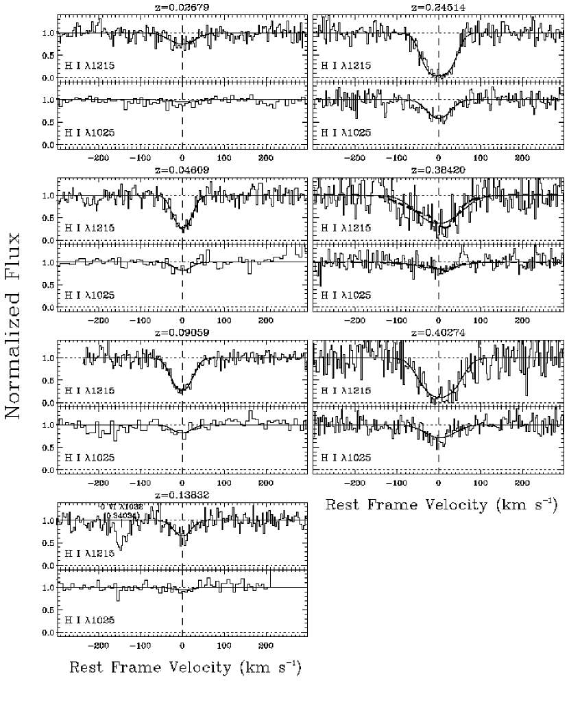
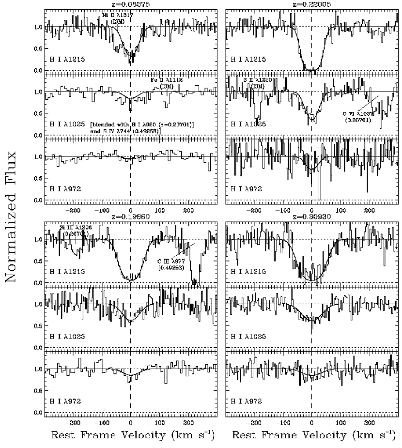
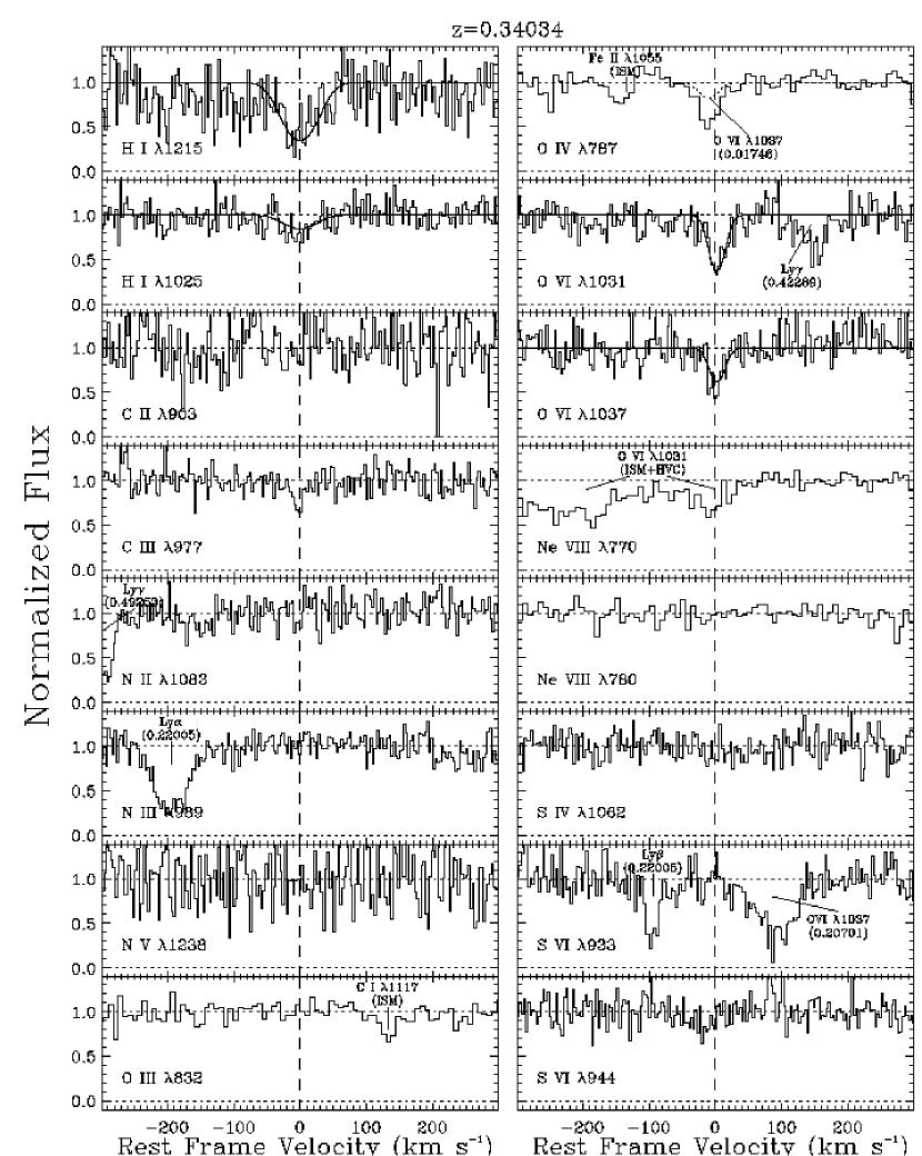
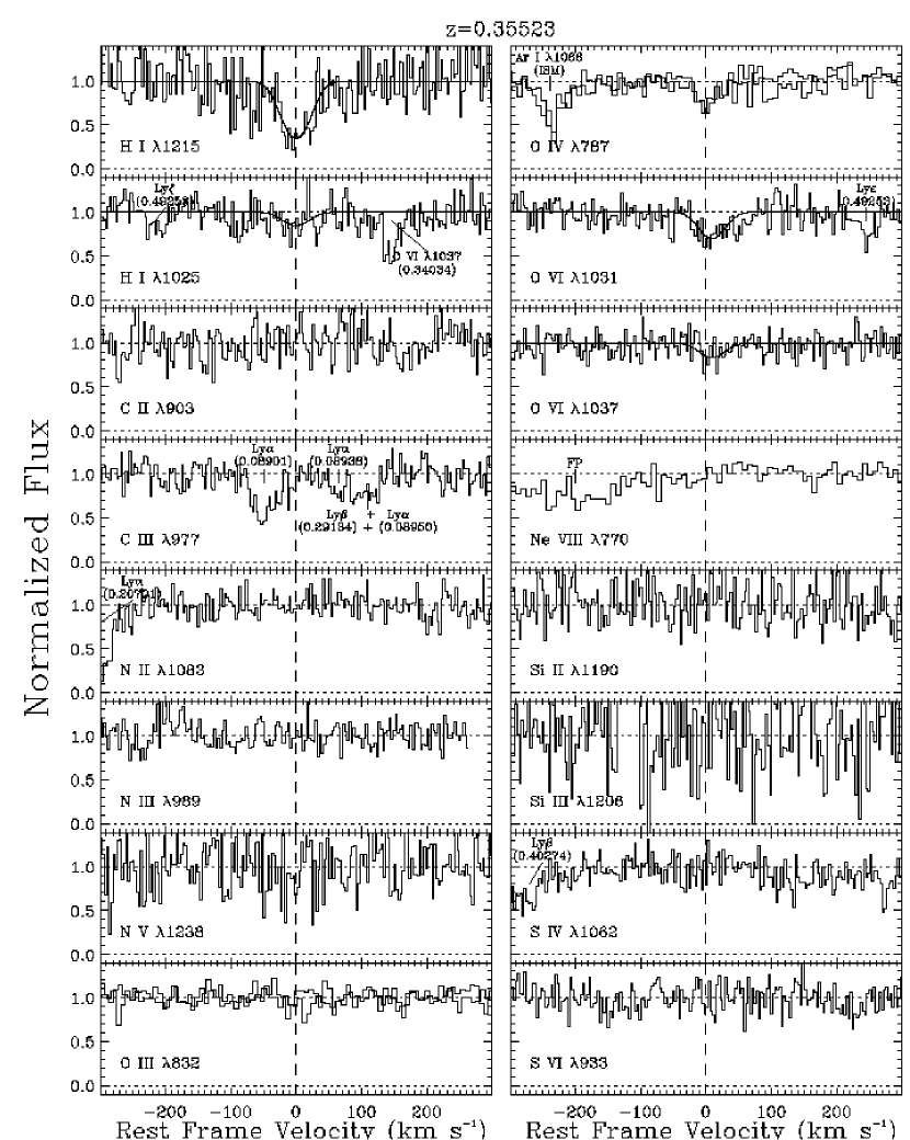
We also fitted the absorption lines with the Voigt component software of Fitzpatrick & Spitzer (1997). In the FUSE band, we assume a Gaussian instrumental spread function with a , while in the STIS band, the STIS instrumental spread function was adopted (Proffitt et al., 2002). Note that to constrain further the fit to the H I absorption, we systematically (except as otherwise stated in Table 3) use non-detected low-order Lyman-series lines (all the lines used in the fit are listed in Table 3 in the line corresponding to the fit result). For this reason, we favored the -values and column densities derived from profile fitting when realized. We note, however, that the results obtained from the moments of the optical depth and profile fitting methods are in agreement to within 1 for most cases. We show the normalized spectra (with the fit to the absorption lines when realized) against the rest-frame velocity of the H I absorbers in Figs. 4 (systems detected only in Ly), 5 (systems detected in Ly and Ly), 6 (systems detected in Ly, Ly, Ly), 7 (system detected in Ly, Ly and Ly, and Ly), and the metal systems in Figs. 8, 9, 10, 11, and 12. See also Figs. 2 and 4 in Savage et al. (2005) for the metal system at . We find several broad H I absorption profiles with . For most of these systems a 2 component fit does not improve significantly the reduced-. The system at appears to have an asymmetric profile in both the Ly and Ly lines, and for this system a 2 component fit looks better by eye but not statistically (see dotted lines in Fig. 5). In the note of Table 3 we give the results of the fit for this system: a combination of broad ( ) and narrow ( ) lines seem to adequately fit the H I profiles. Hence, in any case, a broad component is present. But, only the systems at and 0.27155 are clearly multiple components blended together. We note that several systems are only a separated by less than a few hundreds . We will discuss further these systems in our future paper on the H I in the low redshift IGM (N. Lehner et al. 2006, in prep.).
For all the non-detections we list in Table 3 the 3 upper limits to the rest-frame equivalent width and to the column density by assuming the absorption lines lie on the linear part of the curve of the growth. We adopted the velocity range either from other observed metals or from the Lyman lines if no metals were detected (see Table 3 for more details); except if H I , we set .
Table 4 is a summary table that presents the redshift, the H I column density and Doppler parameter, and the column densities of C III, O III, O IV, O VI, and Ne VIII. The derived H I parameters () and the O VI column densities are from profile fitting. For the other ions, the column density is from AOD (except for the columns of the system at that resulted from profile fitting, see Savage et al. 2005).
3.3 Possible Misidentification
While we have done our best to identify properly all the absorption features in the spectrum of HE 0226–4110, misidentifications are possible because we do not have access to the full redshift path to HE 0226–4110. The highest redshift at which Ly is detectable is (see §3.4). Thus, Ly between 0.423 and 0.495 is not detectable and could produce Ly between 1458.6 and 1533.4 Å, i.e. between redshift and (Ly cannot be Ly because that would imply .) The following systems are thus potentially affected : , 0.20701, 0.22005, 0.22099, 0.23009, 0.23964, 0.24514. However, the 0.19860, 0.20055, 0.20701, 0.22005 and 0.24514 systems have Ly and Ly. The system at would correspond to Ly at . At , a feature at 1383.822 Å (marked as Ly at in Fig. 3) could possibly be identified with Ly, but the measured H I column densities for Ly and are discrepant by 0.25 dex. Hence, the system at is most likely to be Ly too. The remaining Ly systems at , 0.23009, 0.23964 could actually be Ly at , 0.45799, 0.46931, respectively. Those are marked by “!” in Tables 3 and 4.
We note that the O VI system could be Ly at and 0.21756, or Ly at and 0.44314. However, the derived physical parameters appear to match very well the atomic properties of the O VI doublet (see Table 3 and Fig. 12). We also note that several cases where O VI is observed without Ly or Ly are reported in T. M. Tripp et al. (2006, in prep.): (i) O VI observed without H I is detected in four cases in associated systems; (ii) the intervening system at toward PKS 0405–125 has strong O VI with no Ly,; (iii) for PKS 1302–102 at there is an excellent O VI doublet detection and very low ( sigma) significance Ly and no Ly detection; (iv) there are several cases in the more complex H I systems where there is clearly detected O VI well displaced in velocity from the H I absorption. Therefore, the system is likely to be an O VI system, but we would need a FUV spectrum that covers the wavelength up to 1850 Å to have a definitive answer. We will therefore treat this system in the paper as a tentative O VI system and this system is also marked by “!” in Tables 3 and 4.
We finally note that there may be O VI at and 0.29134. For the system at , O VI 1037 is identified as Ly at , but the O VI 1032 appears weaker than expected and is not . Therefore, we do not report these features as O VI. For the system at , O VI would be shifted by with respect to H I. Neither of the O VI lines are , and therefore we elected not to include them as reliable detections.
3.4 Unblocked-Redshift Path
We will need later (see §5.2) the unblocked redshift path for several species under study. The maximum redshift path available for Ly is set by the maximum wavelength available with STIS E140M, which is 1729.5 Å, corresponding to . Note that the redshift of HE 0226–4110 is larger, . The blocked redshift interval arising from interstellar lines, other intervening intergalactic absorption lines, and the gaps existing in the wavelength coverage is . The unblocked redshift path for H I is .
For O VI, we follow a similar method but we note that O VI can arise without detection of H I (see §3.3) since we are not covering the whole wavelength range for Ly. We therefore do not restrict the O VI redshift path to H I. We also restrict the part of spectrum to where a 3 limit integrated over is mÅ. Therefore the STIS spectrum between 1182 Å to 1225 Å and above 1565 Å was not used (at Å, the FUSE spectrum was used to search for O VI). The unblocked redshift path for O VI is . In principle the unblocked redshift path is larger for the C III and the EUV lines but because they are much more difficult to detect (single line or weaker doublet), we adopt for C III, O II, O III, O IV, and Ne VIII the redshift path of O VI corrected for any blocked redshift interval arising from interstellar lines and other intervening intergalactic absorption lines at Å. We also consider only wavelengths with Å for those lines because at smaller wavelengths the spectrum is too confused with the ISM Lyman series absorption lines. This would give an unblocked redshift path for O II and O III of about 0.350 and for O IV and Ne VIII of 0.283.
4 Physical Conditions in the Metal-Line Absorbers
One of the main issues with the detection of O VI absorbers is given the measurements of the different species, can we distinguish between photoionization and collisional ionization, between warm and hot gas? This is a fundamental question because to be able to estimate O VI) in the WHIM, we need to know how much of the observed O VI is actually in shock-heated hot gas rather than in cooler photoionized gas. For each of the observed absorbers we will first investigate if a photoionization equilibrium model is a viable option for the source of ionization. We will then consider other sources, in particular collisional ionization equilibrium (CIE) models from Sutherland & Dopita (1993).
4.1 Photoionization
In the IGM, the EUV ionizing radiation field can be energetic enough to produce high ions in a very low density gas with a long path length. To evaluate whether or not photoionization can explain the observed properties of the O VI absorbers, we have run the photoionization equilibrium code CLOUDY (Ferland et al., 1998) with the standard assumptions, in particular that there has been enough time for thermal and ionization equilibrium to prevail. We model the column densities of the different ions through a slab illuminated by the Haardt & Madau (1996) UV background ionizing radiation field from QSOs and AGNs appropriate for the redshift of a given system. The models assume solar relative heavy element abundances from Grevesse & Sauval (1998), but with the updates from Holweger (2001) for N and Si, from Allende Prieto et al. (2002) for C, and from Asplund et al. (2004) for O and Ne (see Table 5 in Savage et al. 2005, and see also §5.3 for Ne). With these assumptions, we varied the metallicity and the ionization parameter ( H ionizing photon density/total hydrogen number density [neutral + ionized]) to search for models that are consistent with the constraints set by the column densities of the various species and the temperature given by the broadening of an absorption line:
| (1) |
(where is atomic weight of a given chemical element). The temperature is only an upper limit because mechanisms other than thermal Doppler broadening could play a role in the broadening of the line.
The System at :
The absorber system at (see Fig. 8) has the lowest redshift of all absorbers in our HE 0226–4110 data. It is detected in Ly, C IV (), and O VI 1031 (, O VI 1037 is blended with O IV at ). The profile fit to H I implies K. The kinematics appear to be simple with all the different species detected at the same velocity within . These species may therefore arise in the same ionized gas. To investigate this possibility we ran CLOUDY models with H I. We estimated that a CLOUDY model with a solar abundance could reproduce the observed measurements of H I, C IV and O VI and the limits on C III and N V (see Fig. 13). The physical parameters are tightly constrained by the O VI column density, with the ionization parameter , the total H density cm-3. The corresponding cloud thickness is about 17 kpc and the total hydrogen column density cm-2. The gas temperature is K, similar to the temperature implied by the broadening of the narrow H I line. These properties are reasonable for a nearby IGM absorber: photoionization is a likely source of ionization for the system at
The System at :
This system has the highest total H I column density. It is detected in several H I Lyman series lines and in many lines of heavier elements in a variety of ionization stages, with in particular the detection of Ne VIII. This is the most complex metal-line system in the spectrum with at least two velocity-components in H I and one should refer to Savage et al. (2005) for detailed analysis and interpretation of this system. This system has a metallicity of dex and has multiple phases, including photoionized and shock-heated gas phases.
The System at :
This system has absorption seen in Ly, Ly, C III, O IV, and O VI (see Fig. 10). The velocity-centroids of these species agree well within the errors, and therefore a single-phase photoionized model may explain the observed column densities of the various observed species. We ran the CLOUDY models with . We estimated that a simple photoionized model with a 1/2 solar abundance could reproduce the observed measurements of H I, C III and O VI and the limits (see Fig. 14, we did not plot the limits for clarity). The physical parameters are tightly constrained by the O VI and C III column densities, with the ionization parameter , the total H density cm-3. At higher or lower metallicity, the models cannot reproduce uniquely all the column densities of the various observed ions. The corresponding cloud thickness is about 40 kpc and the total hydrogen column density cm-2. The profile fit to H I implies K, which is compatible with the gas temperature K derived by CLOUDY at with no additional non-thermal broadening.
In conclusion, the observed simple kinematics and the column densities can be explained by a photoionization model with a 1/2 solar metallicity, and . Therefore, photoionization can be a dominant process for this system too.
The System at :
This system is the third most complex metal-system toward HE 0226–4110, with absorption seen in Ly, Ly, O IV, and O VI. The LiF 2A channel suggests a nearly 3 feature for O III, but a comparison of LiF 2A and LiF 1B shows it is only a noise feature (see Fig. 11). The O IV feature is, however, real since it is present in both channels, LiF 1A and LiF 2B. The profiles of Ly and Ly are noisy and do not suggest a multicomponent structure. H I and O IV align very well, but the O VI profile appears to be more complex. The deeper part of the O VI 1031 trough aligns well with O IV, but there is a positive velocity wing, a 3 feature ( mÅ) at +50 . This feature could be an extra O VI component or a weak intervening Ly absorption. The S/N is not high enough to really understand the full complexity of the O VI profile. We therefore treated O VI as being co-existent with O IV, and in particular we use the O IV profile to define the velocity range for integration of the O VI absorption lines.
We ran a CLOUDY simulation with . The total column density of O IV and O VI and the limit on C III can be satisfied simultaneously in the photoionization model for a very narrow range of metallicity near at the given . At a higher metallicity () the O VI and C III column density models diverge, and at a lower metallicity, the models do not predict enough O IV. In Fig 15, we show the CLOUDY model with 0.28 solar metallicity. The small error on O VI allows only a very narrow range of ionization parameters at ( cm-3). The corresponding cloud thickness is about 40 kpc and the total hydrogen column density cm-2. The gas temperature is K. The Doppler parameter of H I implies that K, which is compatible with derived in the CLOUDY simulation.
For the system at , a photoionization model with 0.28 solar metallicity and can explain the measured O IV and O VI column densities and the limit on C III).
The System at :
This system is only detected in both O VI lines (see Fig. 12) and could be misidentified (see §3.3). But, although the O VI 1031 line is confused with a spike due to hot pixels, both the strength and the separation of the absorption lines match the atomic parameters of the O VI doublet. No H I is found associated with this system, but the wavelength range only allows us to access Ly. Because O VI 1031 is blended with an emission artifact, it is not clear if the O VI profile has only one or more components. The negative velocity part of the profile of O VI 1031 where the line is not contaminated by the instrumental spike suggests a rather smooth profile. The O VI 1037 absorption is noisy and too weak to indicate if more than one component is needed. We therefore fitted the O VI lines with one component and removed the apparent emission feature from the fit. We note that if the fit is made using O VI 1037 alone, the parameters are consistent with those of the fit to the doublet. The errors on the -value may be larger than the formal errors presented in Table 3. The fit to the O VI absorption lines yields , implying K.
We explored the possibility that this system may be principally photoionized by the UV background. Since we do not know the amount of H I for this absorber and have only O VI, the results remain uncertain. For a wide variety of inputs (H I, and ), the observed O VI column density can be reproduced with a reasonable ionization parameter of or smaller and a cloud thickness less than 100 kpc. The broadening of the O VI profiles is non-thermal since photoionization models give a gas temperature of K. The Hubble flow broadening appears also negligible in most cases. We note that none of the other column density limits constrain the model further.
4.2 Collisional Ionization
We showed above that the O VI systems along with the ancillary ions can be modeled by photoionization alone, except for the system at described by Savage et al. (2005) for which O VI clearly traces hot gas. If photoionization is the dominant source of ionization of these systems, the broadening of O VI and the other metal-lines is dominated by non-thermal broadening or substructure may be present since the temperature of the photoionized gas is typically a few K. For H I, however, there is little room for other broadening mechanisms since . We note that O VI is detected at in the FUSE spectrum, which has an instrumental broadening of about . For this system, it is not possible to determine whether is smaller than its instrumental width. Within the errors, the broadening of the line can be reconciled with a broadening from nearly purely thermal motions. The other O VI systems lie in the STIS spectrum, but the S/N of those data is not good enough to distinguish between single and multiple absorption components. In particular, we note the complexity of the O VI profile at .
The broadening of the O VI lines (and C IV and O IV when detected) implies temperatures of a few K if the broadening is purely thermal. At these temperatures, collisional ionization can be an important source of ionization (Sutherland & Dopita, 1993). If CIE applies, these systems must be multi-phase since the observed narrow H I absorptions cannot arise in hot gas. Therefore, there is a large degree of uncertainty in any attempt to derive parameters from CIE models since the fraction of O VI or other ions arising in photoionized or collisionally ionized gas is unknown, and the kinematics do not allow a clear separation of gas phases within different ionization origins. With this caveat and making the strong assumption that the metal-ions are not produced in photoionized gas, we review now if CIE could match the observed column densities of the metal-line systems:
The System at :
The broadening of O VI implies K (with a large uncertainty) if it is purely thermal. The limit for is very close to the peak temperature for O VI in collisional ionization equilibrium ( K; Sutherland & Dopita, 1993). The ratios is compatible with the highly ionized gas being in collisional ionization equilibrium at K, close to the thermal broadening for O VI. But implies that N must be subsolar because CIE predicts a fraction of 0.2 at . At this temperature H I for pure thermal broadening; such a broad component could be superposed on the narrow H I absorption and hidden in the noise of the spectrum. To constrain the H I column density of the broad component, we fit the Ly profile simultaneously with both narrow and broad lines. For the broad component we fix H I and H IO VI). The parameters are free to vary for the narrow component. We find a fit with a very similar reduced- as that of the one component fit, giving H I. In Fig. 16, we show the fit to the Ly line for H I. In CIE, at , the logarithmic ratio of O VI fraction to H I fraction is (Sutherland & Dopita, 1993) and the solar oxygen abundance is (Asplund et al., 2004), implying [O/H if H I and [O/H if H I. Yet, the non-detection of N V implies a N/O ratio less than 0.4 times solar. A low N/O ratio has recently been observed in a solar metallicity environment in the low- IGM toward PHL 1811 (Jenkins et al., 2005). Therefore, this system could be collisionally ionized.
The System at :
We find O VIO IV). In CIE, O IV and O VI have the same ionic fraction at K, which corresponds to the thermal broadening of these lines within . The fact that is consistent with this temperature. A temperature of K implies H I if the broadening is purely thermal. Such a broad component could be hidden in the noise of the spectrum. The blue part of the Ly spectrum may indicate the presence of a broad wing (see Fig. 10), but the total recovery of the flux on the red part of the Ly spectrum indicates that the features within the blue wing are not part of the main H I absorption. While we can force a broad Ly in the observed profile in the same way that we did for the system at , the data do not warrant it. CIE may be viable for this system, but higher quality data are needed to check this. The photoionization model with the adopted parameter predicts N V, while CIE predicts N V (assuming a solar abundance). An increase in the S/N by about a factor 3 would provide a good 3 limit on N V and several other species which would allow a discrimination between these models.
The System at :
The same discussion applies for this system as for the system since the ionic ratios are similar. Higher S/N data would provide better constraints on N V here as well. However, the broadening of the O IV and O VI lines are more consistent with K. Therefore either there is substructure in the profile as the complexity of the O VI 1031 profile may suggest, or non-thermal broadening is present if CIE applies.
The System at :
The fit to the O VI absorption lines yields , implying K. In CIE at K, we should find Ne VIII if the relative abundance of Ne and O is solar. Our 3 limit for Ne VIII suggests a much smaller column density, less than 13.57 dex. If the temperature is K (corresponding to a thermal -value for O VI of about 25 ), the ratio of Ne VIII to O VI would be consistent with the observed ratio (this would also fit the ratio limit for O IV to O VI). If the gas is hot, either the profiles may be more complicated, the broadening not solely thermal, or the abundance of Ne to O not solar. We note that the AOD -value of O VI 1037 is less than 2 from 25 , where Ne VIIIO VI.
The System at
This absorber has not been discussed yet because no O VI is detected and there is only a tentative measurement of C III. It has also a broad H I component, potentially tracing hot gas. It is seen in Ly and Ly, with Ly hidden by interstellar Si II 1193 (see Table 3 and Fig. 9). O III is confused with H2 (see Table 3). There is a detection of C III in LiF 1A. The data from LiF 1B have lower S/N than LiF 2A and imply a 2.9 upper limit of 12.51 dex for C III, although one pixel is aligned with C III in LiF 2A (see Fig 9). Within the errors, H I and C III have compatible redshifts. The profile of H I is very well fitted with a single Gaussian with . If the broadening is purely thermal, this would imply H I K. This is the only broad H I system for which a metal ion is (tentatively) detected along this line of sight. Generally, O VI is a more likely ion to associate with broad H I (Richter et al., 2004; Sembach et al., 2004), but ions in lower ionization stages can constrain the metallicity of broad Ly absorbers as well. We find , if CIE and pure thermal broadening apply.
4.3 Summary of the Origin of the O VI systems in the Spectrum of HE 02260-4110
In summary, the O VI systems at , 0.34034, 0.35523, 0.42660 can be explained by photoionization models. In Table 5, we summarize the basic properties of the observed O VI systems assuming photoionization and the possible origins of these systems. The broadening of the metal lines appears to be mostly non-thermal if solely photoionization applies or there may be unresolved sub-structure buried in the noise of the spectrum. Only the system at described by Savage et al. (2005) appears to be clearly multiphase with photoionized and collisionally ionized gas. The ionic ratios observed in the system at can be reconciled with a single CIE model if the relative abundances are non-solar. For the other systems, CIE is possible with current constraints. In particular, only a little non-thermal broadening would be needed to explain the broadening of the metal lines. Higher S/N FUV spectra would provide better understanding of the shape and kinematics of the observed profiles and access to other key elements such as N V.
5 Implications for the Low Redshift IGM
5.1 Discriminating between Photoionization and Collisional Ionization
The analysis in §4 shows that it is difficult to clearly differentiate between photoionization and collisional ionization for several of the metal-line systems. Savage et al. (2005) showed that the system at consists of a mixture of photoionized and collisionally ionized gas. This is the only system along this line of sight for which O VI cannot be explained by photoionization. We showed that the system at can be collisionally ionized if N/O is sub-solar, but the observed column densities can also be explained by a simple photoionization model with relative solar abundance. For the O VI systems at and 0.35523 and the tentative O VI system at , photoionization is also the likely source of ionization, although collisional ionization cannot be ruled out.
If the photoionization dominates the ionization in a large fraction of the O VI systems, estimates of the baryonic density of the WHIM as traced by O VI would need to be reduced by a similarly large factor (a factor 6 for the HE 0226–4110 line of sight). The recent observations in the FUV of the lines of sight toward H 1821+643 (Tripp et al., 2001), PG 1116+215 (Sembach et al., 2004), PG 1259+593 (Richter et al., 2004), and PKS 0405–123 (Prochaska et al., 2004) have similarly shown that the O VI systems are complex, with a mix of photoionized, and collisionally ionized systems.
Prochaska et al. (2004) noted a general decline of the photoionization parameter estimated in the CLOUDY model with increasing observed H I column density. Davé et al. (1999) found that H I for the low- Ly absorbers. Assuming that the H I ionizing intensity is constant gives H I (Prochaska et al., 2004). To check if this trend holds with more data and in particular to check if the O VI systems that could be explained by both photoionization and CIE deviate from this trend, in Fig. 17 we combine our results summarized in Table 5 for the photoionized O VI systems with results from Prochaska et al. (2004), Richter et al. (2004), Savage et al. (2002), and Sembach et al. (2004). We show in Table Low Redshift Intergalactic Absorption Lines in the Spectrum of HE 0226–411011affiliation: Based on observations made with the NASA-CNES-CSA Far Ultraviolet Spectroscopic Explorer. FUSE is operated for NASA by the Johns Hopkins University under NASA contract NAS5-32985. Based on observations made with the NASA/ESA Hubble Space Telescope, obtained at the Space Telescope Science Institute, which is operated by the Association of Universities for Research in Astronomy, Inc. under NASA contract No. NAS5-26555. the redshift, , and H I column density. A linear fit using a least squares fit to the data gives (we did not include the peculiar O VI system at toward PKS 0405–123 where the very weak Ly is offset from the metal-line transitions, see Prochaska et al. 2004; including this system would change the slope to ). For the fit we treated the lower limit of toward PKS 0405–123 as an absolute measure, but excluding this limit from the fit would not change the result. The solid curve in Fig. 17 shows the fit. While the slope of is close to the predicted slope of from the numerical simulations (Davé et al., 1999; Davé & Tripp, 2001), the simulations appear to provide an upper limit to this relation (see dotted line in Fig. 17). Note that metal-line systems with no O VI do not seem to follow this correlation. For example the system at toward 3C 273 gives H I and (Tripp et al., 2002), and the system at gives H I and (Sembach et al., 2004): both systems are very much below the distribution of the data plotted in Fig. 17. Although the correlation could be somewhat fortuitous for the O VI systems that can be explained by both photoionization and CIE origins, it would have to occur for all these systems (e.g., 2 systems presented in this paper, and the system at toward PG 0953+415 in Savage et al. 2002). This may favor photoionization for the O VI systems that can be fitted by both photoionization and CIE models.
So far, we have mainly considered photoionization and CIE models to explain the observed O VI systems. However, if the gas is hot (between and K) and dense enough, it should cool rapidly since this is the temperature range over which the cooling of an ionized plasma is maximal (Sutherland & Dopita, 1993). O VI is the dominant coolant in this temperature range. Heckman et al. (2002) investigated the non-equilibrium cooling of O VI and computed the relation between (O VI) and (O VI) expected for radiatively cooling gas at temperatures of and K. Considering the 4 IGM sight lines that have now been fully analyzed (HE 0226–4110, this paper; PKS 0405–123, Williger et al. 2005; PG 1116+215, Sembach et al. 2004; PG 1259+593, Richter et al. 2004), we plot in Fig. 18 the column density against the observed width for O VI absorption systems seen along these lines of sight. Most of the data lie between the -range [10,35] and -range [13.5,14.1] with a large scatter. Considering data outside these ranges, there is a general trend of the O VI column increasing with increasing O VI width, as observed in the Galaxy, Small and Large Magellanic Clouds (Savage et al., 2003). There is no obvious separation in Fig. 18 between systems that could be photoionized or collisionally ionized. In this figure, we also reproduce Heckman et al.’s radiative cooling models for and K and the (O VI) linear regime ( , see Heckman et al.). Their models can reproduce the observed distribution. Heckman et al. (2002) also computed the column densities of several ancillary species. We reproduce the observed and predicted ratios of O IV/O VI, Ne VIII/O VI, and S VI/O VI in Table 7. Generally, their models produce too much Ne VIII. For O IV and S VI, the comparison may be more difficult because photoionization may play a role, but photoionization can also produce O VI if the IGM has a very low density. So while these cooling models can reproduce the distribution of (O VI) and (O VI), they generally fail to predict observed ionic ratios, especially Ne VIII/O VI. The pure isobaric model is always ruled out, as it predicts a O IV/O VI ratio that is too low. Note that these models assume solar relative elemental abundances.
In summary, our results show that for 1 out of 5 O VI systems toward HE 0226–4110, collisional ionization is the likely origin of the O VI. For the 4 other systems, comparison of the ionic ratios and the kinematics of the ionic profiles does not yield a single solution for the origin of the O VI. We note that and (H I) of these systems correlate and follow the same distribution as pure photoionized O VI systems, suggesting that photoionization could be the origin of these O VI systems. To better understand the basic properties of the IGM in the low redshift universe, observations with high S/N data are needed. At high redshift, data with S/N of 100 per 7 resolution element have answered many fundamental questions that remained unanswered with low quality data. While in the near future FUV spectra will not have the quality of the current optical data, S/N of 50 or higher could be achieved on bright QSOs with the Cosmic Origin Spectrograph (COS) when/if it is installed on the HST.
5.2 Frequency of Occurrence Of Oxygen in Different Ionization Stages
Oxygen is certainly the best metal element for the study of the physical properties of the IGM because it is the most abundant and because it has a full range of ionization stages, from O I to O VIII, accessible to existing spectrographs. While we are far from being able to combine X-ray (O VII, O VIII) lines with FUV lines because of sensitivity and spectral resolution issues, searching for O I to O VI is possible by combining EUV and FUV lines available in the FUSE and STIS wavelength ranges. In Table 8, we summarize the transitions of oxygen observable in the EUV–FUV and the redshift at which these transitions can be observed. Toward HE 0226–4110, we unfortunately miss O V 629 (because the redshift path of HE 0226–4110 is not large enough (O V is detected in the associated system, see Fig. 2). The close match in the oscillator strengths among these ions also allow direct comparisons of lines with similar column density sensitivities (see Table 8).
For the Ly systems detected toward HE 0226–4110 it is almost always possible to search for the associated metal lines, as blending is rarely a problem. The only system where we cannot study O VI is the one at . For all the other systems, we are able to measure the O VI column density or estimate a 3 limit. For 5 absorbers, () O VI 1031 is blended with other IGM or ISM absorptions, so the limits were estimated with O VI 1037. For O III and O IV there are only 8 and 2 systems, respectively, for which we cannot make a measurement because of blending (see Table 4). We do not report estimates for O I and O II because these lines are rarely detected in the Ly forest (they are sometimes detected in the high H I column systems with H I , see Prochaska et al. 2004, Sembach et al. 2004, Tripp et al. 2005). Since no unidentified features with lie at the wavelengths where O I and O II associated with H I are expected, we can confidently say that there are no intervening systems with O I and O II lines in the spectrum of HE 0226–4110.
A useful statistical quantity to use for constraining the ionization of the IGM is the number of intervening systems per unit redshift. For O VI, five intervening systems toward HE 0226–4110 are detected in either one () or both O VI lines (). These 5 systems have mÅ. The number of intervening O VI systems with mÅ per unit redshift is for an unblocked redshift path of 0.450 (see §3.4). This number would be 9 if the tentative system is not included.
There is one definitive detection of O III and there are 3 detections of O IV in the spectrum of HE 0226–4110. Using the redshift path defined in §3.4, and . If we adopt the unblocked redshift path of H I instead of O VI, these numbers do not change significantly. While this sample still suffers from small number statistics, it suggests in the IGM along the HE 0226–4110 sight line. Since the values of of the oxygen lines are similar, the column density limits for these different ions are similar. The ionization potentials of O III and C III are similar and since there are more systems for which we can search for C III, we also report the measurement of the strong C III line () in Table 4. Only for the systems at were we not able to estimate the amount of C III. We find . Richter et al. (2004) reported 4 definitive O VI systems and detection of two O III and O IV systems (one of them not associated with O VI) toward PG 1259+593. Adopting the same procedure as above, toward PG 1259+593, we find . There are 5 reported C III systems against 6 O VI systems along the sight line toward PKS 0405–123 (Prochaska et al., 2004), implying . Along the path to PKS 0405–123, there are 1 O III system and 4 detected O IV systems that imply . Combining these sight lines, we find: .
The general pattern that emerges is that there is a slightly larger number of O IV and O VI systems per unit redshift compared to O III, about the same number of O IV and O VI systems per unit redshift, but a much larger number of O III systems per unit redshift than for O I and O II. The low redshift IGM is more highly ionized than weakly ionized. This is consistent with the picture of the Ly forest consisting mainly of very low density photoionized gas and hot gas. We also note that when O III, O IV, and O VI are detected simultaneously the column densities of these ions generally do not differ by more than a factor 2–3.
5.3 Observations of Ne VIII
Li-like Ne VIII provides a powerful diagnostic of hot gas because in CIE it peaks at K, Ne has a relatively high cosmic abundance ([Ne/H) and the Ne VIII lines have relatively high -values (). In CIE at K, Ne VIIIO VI. For K, Ne VIIIO VI. Savage et al. (2005) discussed the system at in the spectrum of HE 0226–4110 and they reported the first detection of an intervening Ne VIII system in the IGM. The O VI/Ne VIII system arises in hot gas at K. With little contamination from H2 lines and its high redshift path, HE 0226–4110 currently provides the best line of sight to search for Ne VIII. We found, however, only one detection of Ne VIII among the 32 H I systems (excluding the associated system) at redshifts where Ne VIII could be measured. We also searched for pairs of absorption features with the appropriate separation of the Ne VIII doublet, not associated with a Ly feature, and found none. Note that none of the H I systems observed are broad enough to produce a significant fraction of Ne VIII, since the broadest H I implies K.
In Fig. 19a we show the column density limits and measurement for Ne VIII against those of O VI for the HE 0226–4110 line of sight. The upper limits on (Ne VIII) were typically integrated over a velocity range of 80–100 , which corresponds to K if the profile is purely thermally broadened. Fig. 19b shows the relationship of the ratio of the Ne VIII to O VI column with the temperature for the CIE model of Sutherland & Dopita (1993) assuming a solar relative abundance. The circles overplotted on this curve are obtained from the measurements of O VI and measurements or upper limits on Ne VIII obtained toward HE 0226–4110, PKS 0405–123 (Prochaska et al., 2004; Williger et al., 2005), and PG1259+594 (Richter et al., 2004) lines of sight. These data cannot fit the curve at higher temperatures because the observed O VI broadening always implies K, except for the system at . For this system the limit on Ne VIII is too small. If CIE applies along with solar Ne/O, all these data imply K for the O VI systems. Fig. 18 shows that most of the detected O VI systems have column densities dex. Hence, the present observations should be sufficiently sensitive to detect Ne VIII systems with K since most of our limits are less than 13.8 dex (see Fig. 19a). We note that even though at higher temperatures Ne VIIIO VI, the Ne VIII profile would be broadened beyond detection with the current S/N observations. For the O VI system at , the broadening of the O VI absorption favors a high temperature, but no Ne VIII is detected; since the O VI system can be photoionized and non-thermally broadened, a cooler temperature is possible.
Solar reference abundances have changed quite significantly over the recent years for C, O, and Ne. Since Savage et al. (2005) produced the summary of recent solar abundance revisions (see their Table 5), recent helioseismological observations have been used to argue that the Ne abundance given by Asplund et al. (2004) is too low to be consistent with the solar interior (Bahcall et al., 2005). Recently, Drake & Testa (2005) derived Ne/O abundances from Chandra X-ray spectra of solar-type stars and they found Ne/O abundances that are 2.7 times larger than the values reported by Asplund et al. (2004), which alleviates the helioseismology problem. But if the Ne abundance is instead of , it would further complicate the explanation for the low frequency of occurrence of Ne VIII systems. It is still unclear what the definitive value is for the solar Ne abundance, since recent re-analysis of solar spectra still yield a low value (e.g., Young, 2005).
The WHIM at K (where the bulk of the baryons should be formed, according to simulations) remains still to be discovered with EUV–FUV metal-line observations. So far only the X-ray detections of O VII in nearby systems at discussed by Nicastro et al. (2005) imply temperatures of a few K. The non-detection of hot systems with K via Ne VIII may have several explanations and implications. If the O VI systems are mainly photoionized it is not surprising to find very few containing Ne VIII. Assuming that the numerical simulations of the WHIM are correct, the bulk of the WHIM may have a lower metallicity than the gas traced by hot O VI absorbers. Broad Ly absorbers which trace the WHIM appear in some cases to have a 0.01 solar abundance (see §4.2). The relative abundances may not be always solar. Low metallicity environments are known to have relative abundances different than those in the Sun. CIE models may not be a valid representation of the distribution of ions in hot gas in the WHIM, but we note that the non-equilibrium cooling flow models by Heckman et al. (2002) would generally also predict too much Ne VIII (see Table 7). Additional and more sensitive searches for Ne VIII would be valuable for better statistics and a better understanding of the Ne VIII systems, and their frequency of occurrence in the IGM.
5.4 Metallicity of the Low Redshift Metal-Systems
Metallicity is a quantity that is fundamental in obtaining estimates of from metal-line absorbers and following the chemical enrichment of the IGM. A metallicity of 0.1 solar is generally adopted for estimating (e.g., Tripp, Savage, & Jenkins, 2000; Danforth & Shull, 2005), but since , a change in the adopted metallicity can significantly alter the estimated . Table Low Redshift Intergalactic Absorption Lines in the Spectrum of HE 0226–411011affiliation: Based on observations made with the NASA-CNES-CSA Far Ultraviolet Spectroscopic Explorer. FUSE is operated for NASA by the Johns Hopkins University under NASA contract NAS5-32985. Based on observations made with the NASA/ESA Hubble Space Telescope, obtained at the Space Telescope Science Institute, which is operated by the Association of Universities for Research in Astronomy, Inc. under NASA contract No. NAS5-26555. provides recent metallicity estimates via photoionization models of O VI systems in the low redshift IGM. If these systems are primarily photoionized, they are not tracers of the WHIM. But abundance measurements in collisionally gas are generally not reliable. Combining the results in Table 6, we find a median abundance for the photoionized O VI systems of dex solar with a large scatter of dex around this value. Only 4 of 13 systems appear to be either at solar abundance or less than 1/10 solar. If those systems are not taken into account, the metallicity is dex. If the metallicity of the photoionized O VI systems reflects the metallicity of the collisionally ionized O VI systems, derived via O VI would decrease by a factor since .
6 Summary
We present the analysis of the intervening absorption and the interpretation of the metal-line systems in the FUSE and STIS FUV spectra of the QSO HE 0226–4110 (). Due to the low fraction of Galactic ISM molecular hydrogen along this line of sight, HE 0226–4110 provides an excellent opportunity to search for metals associated with the Ly forest. For each Ly absorber, we systematically search for C III, O III, O IV, O VI, and Ne VIII. We also search for O VI and Ne VIII doublets not associated with H I. For each metal-line system detected, we also search for any other metals that may be present. The richest intervening metal-line system along the HE 0226–4110 sight line is at . This system was fully discussed by Savage et al. (2005). We examine the ionic ratios to constrain the ionization mechanisms, the metallicity, and physical conditions of the absorbers using single-phase photoionization and collisional ionization models. We discuss our results in conjunction with analyses of the metal-line systems observed in several other low redshift QSO spectra of similar quality. The main results are as follows:
-
1.
We detect 4 O VI absorbers with rest frame equivalent widths mÅ. A tentative detection at is also reported but this system could be misidentified because Ly cannot be accessed. The number of intervening O VI systems with mÅ per unit redshift is along the HE 0226–4110 line of sight. For 4 of the 5 O VI systems other ions (such as C III, C IV, O III, O IV) are detected.
-
2.
One O VI system at cannot be explained by photoionization by the UV background (see Savage et al. 2005). For the other 4 O VI systems, photoionization can reproduce the observed column densities. However, for these systems, collisional ionization may also be the origin of the O VI. We note that if photoionization applies, the broadening of the metal lines must be mostly non-thermal, but the H I broadening is mostly thermal.
-
3.
Oxygen is particularly useful to study the ionization and physical conditions in the IGM because a wide range of ion states are accessible at FUV and EUV restframe wavelengths, including O I, O II, O III, O IV, O V, and O VI. Our results imply that . The low redshift IGM is more highly ionized than weakly ionized since the transitions for the different oxygen ions have similar values of .
-
4.
Following Prochaska et al. (2004), we confirm with a larger sample that the photoionized metal-line systems have a decreasing ionization parameter with increasing H I column density. The O VI systems that can be explained by both photoionization and collisional ionization follow this relationship. This implies that the systems with photoionization/CIE degeneracy may likely be photoionized.
-
5.
Combining our results with those toward 3 other sight lines, we show that there is a general increase of (O VI) with increasing (O VI) but with a large scatter. The observed distribution of (O VI) and (O VI) can be reproduced by cooling flow models computed by Heckman et al. (2002), but these models fail to reproduce the observed ionic ratios.
-
6.
Combining results for several QSOs we find that the photoionized O VI systems in the low redshift IGM have a median abundance of 0.3 solar, about 3 times the metallicity typically used to derive in the warm-hot IGM gas.
-
7.
Along the path to HE 0226–4110, there is one detection of Ne VIII at that implies a gas temperature of K. We did not detect other Ne VIII systems although our sensitivity should have allowed the detection of Ne VIII in O VI systems at K if CIE applies and Ne/O is solar. Since the bulk of the warm-hot ionized medium (WHIM) is believed to be at temperatures K, the hot part of the WHIM remains to be discovered with FUV–EUV metal-line transitions.
-
8.
This work shows that the origins of the O VI absorption (and the metal-line systems in general) are complex and cause several uncertainties in attempts to estimate from O VI. In particular the O VI ionization mechanism in several cases is indeterminate. High S/N FUV spectra obtained with COS or other future FUV instruments will be needed to solve several of the current observational uncertainties.
References
- Abgrall et al. (1993a) Abgrall, H., Roueff, E., Launay, F., Roncin, J. Y., & Subtil, J. L. 1993a, A&AS, 101, 273
- Abgrall et al. (1993b) Abgrall, H., Roueff, E., Launay, F., Roncin, J. Y., & Subtil, J. L. 1993b, A&AS, 101, 323
- Allende Prieto et al. (2002) Allende Prieto, C., Lambert, D. L., & Asplund, M. 2002, ApJ, 573, L137
- Asplund et al. (2004) Asplund, M., Grevesse, N., Sauval, A. J., Allende Prieto, C., & Kiselman, D. 2004, A&A, 417, 751
- Bahcall et al. (2005) Bahcall, J. N., Basu, S., & Serenelli, A. M. 2005, ApJ, in press
- Bergeron & Herbert-Fort (2005) Bergeron, J., & Herbert-Fort, S. 2005, IAU 199 Conference Proceeding, “Probing Galaxies Through Quasar Absorption Lines”, [astro-ph/0506700]
- Bryan et al. (1999) Bryan, G. L., Machacek, M., Anninos, P., & Norman, M. L. 1999, ApJ, 517, 13
- Burles et al. (2001) Burles, S., Nollett, K. M., & Turner, M. S. 2001, ApJ, 552, L1
- Carswell et al. (2002) Carswell, B., Schaye, J., & Kim, T. 2002, ApJ, 578, 43
- Cen & Ostriker (1999) Cen, R., & Ostriker, J. P. 1999, ApJ 514, 1
- Danforth & Shull (2005) Danforth, C. W., & Shull, J. M. 2005, ApJ, 624, 555
- Davé et al. (1999) Davé, R., Hernquist, L., Katz, N., & Weinberg, D. H. 1999, ApJ, 511, 521
- Davé & Tripp (2001) Davé, R., & Tripp, T. M. 2001, ApJ, 553, 528
- Drake & Testa (2005) Drake, J. J., & Testa, P. 2005, Nature, 436, 525
- Fang et al. (2002) Fang, T., Bryan, G. L., & Canizares, C. R. 2002, ApJ, 564, 604
- Ferland et al. (1998) Ferland, G. J., Korista, K. T., Verner, D. A., Ferguson, J. W., Kingdon, J. B., & Verner, E. M. 1998, PASP, 110, 761
- Fitzpatrick & Spitzer (1997) Fitzpatrick, E. L. & Spitzer, L. J. 1997, ApJ, 475, 623
- Fox et al. (2005) Fox, A. J., Wakker, B. P., Savage, B. D., Tripp, T. M, Sembach, K. R., & Bland-Hawthorn, J. 2005, ApJ, 630, 332
- Fukugita et al. (1998) Fukugita, M., Hogan, C. J., & Peebles, P. J. E. 1998, ApJ, 503, 518
- Ganguly et al. (2005) Ganguly, R., Sembach, K. R., Tripp, T. M., & Savage, B. D., Wakker, B. P. 2005, ApJ, submitted
- Grevesse & Sauval (1998) Grevesse, N., & Sauval, A. J. 1998, Space Science Reviews, 85, 161
- Haardt & Madau (1996) Haardt, F., & Madau, P. 1996, ApJ, 461, 20
- Heckman et al. (2002) Heckman, T. M., Norman, C. A., Strickland, D. K., & Sembach, K. R. 2002, ApJ, 577, 691
- Hernquist et al. (1996) Hernquist, L., Katz, N., Weinberg, D. H., & Jordi, M. 1996, ApJ, 457, L51
- Holweger (2001) Holweger, H. 2001, AIP Conf. Proc. 598: Joint SOHO/ACE workshop ”Solar and Galactic Composition”, 598, 23
- Jenkins et al. (2005) Jenkins, E. B., Bowen, D. V., Tripp, T. M., & Sembach, K. R. 2005, ApJ, 623, 767
- Morton (2003) Morton, D. C. 2003, ApJS, 149, 205
- Moos et al. (2000) Moos, H. W., et al. 2000, ApJ, 538, L1
- Nicastro et al. (2005) Nicastro, F., et al. 2005, Nature, 433, 495
- Penton et al. (2004) Penton, S. V., Stocke, J. T., & Shull, J. M. 2004, ApJS, 152, 29
- Prochaska et al. (2004) Prochaska, J. X., Chen, H., Howk, J. C., Weiner, B. J., & Mulchaey, J. 2004, ApJ, 617, 718
- Proffitt et al. (2002) Proffitt, C., et al. 2000, STIS Instrument Handbook, v6.0, (Baltimore:STScI)
- Rasmussen et al. (2003) Rasmussen, A., Kahn, S. M., & Paerels, F. 2003, ASSL Vol. 281: The IGM/Galaxy Connection. The Distribution of Baryons at z=0, 109
- Rauch et al. (1997) Rauch, M., et al. 1997, ApJ, 489, 7
- Richter et al. (2005) Richter, P., Savage, B. D., Sembach, K. R., & Tripp, T. M. 2005, A&A, in press [astro-ph/0509539]
- Richter et al. (2004) Richter, P., Savage, B. D., Tripp, T. M., & Sembach, K. R. 2004, ApJS, 153, 165
- Sahnow et al. (2000) Sahnow, D. J., et al. 2000, ApJ, 538, L7
- Savage et al. (2005) Savage, B. D., Lehner, N., Wakker, B. P., Sembach, K. R., & Tripp, T. M. 2005, ApJ, 626, 776
- Savage & Sembach (1991) Savage, B. D., & Sembach, K. R. 1991, ApJ, 379, 245
- Savage et al. (2003) Savage, B. D., et al. 2003, ApJS, 146, 125
- Savage et al. (2002) Savage, B. D., Sembach, K. R., Tripp, T. M., & Richter, P. 2002, ApJ, 564, 631
- Sembach & Savage (1992) Sembach, K. R. & Savage, B. D. 1992, ApJS, 83, 147
- Sembach et al. (2003) Sembach, K. R., et al. 2003, ApJS, 146, 165
- Sembach et al. (2004) Sembach, K. R., Tripp, T. M., Savage, B. D., & Richter, P. 2004, ApJS, 155, 351
- Spergel et al. (2003) Spergel, D. N., et al. 2003, ApJS, 148, 175
- Sutherland & Dopita (1993) Sutherland, R. S. & Dopita, M. A. 1993, ApJS, 88, 253
- Tripp et al. (2004) Tripp, T. M., Bowen, D. V., Sembach, K. R., Jenkins, E. B., Savage, B. D., & Richter, P. 2004, ”Astrophysics in the Far Ultraviolet: Five Years of Discovery with FUSE”, [astro-ph/0411151]
- Tripp et al. (2001) Tripp, T. M., Giroux, M. L., Stocke, J. T., Tumlinson, J., & Oegerle, W. R. 2001, ApJ, 563, 724
- Tripp et al. (2005) Tripp, T. M., Jenkins, E. B., Bowen, D. V., Prochaska, J. X., Aracil, B., & Ganguly, R. 2005, ApJ, 619, 714
- Tripp et al. (1998) Tripp, T. M., Lu, L., & Savage, B. D. 1998, ApJ, 508, 200
- Tripp & Savage (2000) Tripp, T. M. & Savage, B. D. 2000, ApJ, 542, 42
- Tripp, Savage, & Jenkins (2000) Tripp, T. M., Savage, B. D., & Jenkins, E. B. 2000, ApJ, 534, L1
- Tripp et al. (2002) Tripp, T. M., et al. 2002, ApJ, 575, 697
- Verner, Verner, & Ferland (1996) Verner, D. A., Verner, E. M., & Ferland, G. J. 1996, Atomic Data Nucl. Data Tables, 64, 1
- Wakker (2005) Wakker, B. P. 2006, ApJ, in press [astro-ph/0512444]
- Wakker et al. (2003) Wakker, B. P., et al. 2003, ApJS, 146, 1
- Weinberg et al. (1997) Weinberg, D. H., Miralda-Escude, J., Hernquist, L., & Katz, N. 1997, ApJ, 490, 564
- Williger et al. (2005) Williger, G. M., Heap, S. R., Weymann, R. J., Dave, R., Ellingson, E., Carswell, R. F., Tripp, T. M., & Jenkins, E. B. 2005, ApJ, in press [astro-ph/0505586]
- Young (2005) Young, P. R. 2005, A&A, 444, L45
| ID | Date | Exp. Time |
|---|---|---|
| (ks) | ||
| O6E107010 | 2002-12-25 | 2.1 |
| O6E107020 | 2002-12-26 | 3.0 |
| O6E107030 | 2002-12-26 | 3.0 |
| O6E108010 | 2002-12-26 | 2.1 |
| O6E108020 | 2002-12-26 | 3.0 |
| O6E108030 | 2002-12-26 | 3.0 |
| O6E109010 | 2002-12-26 | 2.1 |
| O6E109020 | 2002-12-27 | 3.0 |
| O6E109030 | 2002-12-27 | 3.0 |
| O6E110010 | 2002-12-29 | 2.1 |
| O6E110020 | 2002-12-29 | 3.0 |
| O6E110030 | 2002-12-29 | 3.0 |
| O6E111010 | 2002-12-31 | 2.1 |
| O6E111020 | 2002-12-31 | 3.0 |
| O6E111030 | 2003-01-01 | 3.0 |
| O6E111040 | 2003-01-01 | 3.0 |
| Total |
| ID | Date | CALFUSE | Mode | Flux(1A) | Flux(2B) | Flux(Comb.) | 1A)a | 1B)a | 2A)a | 2B)a |
|---|---|---|---|---|---|---|---|---|---|---|
| cgs | cgs | cgs | (ks) | (ks) | (ks) | (ks) | ||||
| P2071301 | 2000-12-12 | v2.1.6 | 2.60 | 2.60 | 2.59 | 11.0 (8.4) | 11.0 (8.4) | 11.0 (8.4) | 11.1 (8.4) | |
| P1019101 | 2001-10-03 | v2.1.6 | FP-SPLIT | 2.57 | 2.73 | 2.62 | 50.3 (37.9) | 50.1 (37.9) | 50.0 (37.9) | 49.9 (38.0) |
| P1019102 | 2002-11-15 | v2.4.0 | FP-SPLIT | 2.44 | 2.06 | 2.30 | 14.5 (11.1) | 14.5 (11.0) | 14.5 (11.0) | 14.5 (11.1) |
| P1019103 | 2002-11-16 | v2.4.0 | FP-SPLIT | 2.45 | 2.19 | 2.35 | 18.9 (14.7) | 18.9 (14.7) | 18.9 (14.7) | 18.9 (14.7) |
| P1019104 | 2002-11-17 | v2.4.0 | FP-SPLIT | 2.57 | 2.39 | 2.50 | 18.1 (10.5) | 18.1 (10.5) | 18.1 (10.5) | 18.1 (10.5) |
| D0270101 | 2003-09-01 | v2.4.0 | 3.06 | 2.80 | 2.97 | 23.9 (12.5) | 24.7 (12.6) | 23.9 (12.4) | 23.9 (12.5) | |
| D0270102 | 2003-09-03 | v2.4.0 | 3.08 | 2.98 | 3.05 | 39.9 (19.2) | 39.4 (19.2) | 37.6 (19.1) | 37.3 (19.1) | |
| D0270103 | 2003-10-31 | v2.4.0 | 3.25 | 3.16 | 3.22 | 16.8 (11.9) | 16.8 (12.0) | 17.0 (12.0) | 17.1 (12.0) | |
| Total | 193.5 (126.1) | 193.5 (126.2) | 191.0 (126.0) | 190.7 (126.2) |
Note. — The first number is the total exposure time. The night-only exposure time is in parenthesis.
| Species | Method | Instrument | ||||||
|---|---|---|---|---|---|---|---|---|
| (Å) | (mÅ) | () | () | (dex) | () | |||
| (1) | (2) | (3) | (4) | (5) | (6) | (7) | (8) | (9) |
| H I 1215 | 1236.944 | AOD | STIS | |||||
| H I 1215,1025 | 1236.944 | FIT | STIS,LiF 2B | |||||
| C II 1036 | 1054.473 | 3 | LiF 1A | |||||
| C III 977 | 994.118 | 3 | LiF 1A | |||||
| C IV 1548 | 1575.289 | AOD | STIS | |||||
| C IV 1550 | 1577.909 | AOD | STIS | |||||
| C IV 1548,1550 | FIT | STIS | ||||||
| N V 1242 | 1264.554 | 3 | STIS | |||||
| O VI 1031 | 1049.964 | AOD | LiF 1A | |||||
| O VI 1031 | 1049.990 | FIT | LiF 1A | |||||
| Si II 1260 | 1282.480 | 3 | STIS | |||||
| Si III 1206 | 1227.614 | 3 | STIS | |||||
| Si IV 1393 | 1418.146 | 3 | STIS | |||||
| H I 1215 | 1248.274 | AOD | STIS | |||||
| H I 1215,972 | FIT | STIS, LiF 1A | ||||||
| C III 977 | 1003.224 | 3 | LiF 1A | |||||
| O VI 1031 | 1059.602 | 3 | LiF 1A | |||||
| H I 1215 | 1265.768 | AOD | STIS | |||||
| H I 1215,1025 | FIT | STIS | ||||||
| C III 977 | 1017.283 | 3 | LiF 1A | |||||
| O VI 1031 | 1074.452 | 3 | LiF 1A | |||||
| H I 1215 | 1270.801 | AOD | STIS | |||||
| H I 1215,1025 | FIT | STIS | ||||||
| C III 977 | 1021.328 | 3 | LiF 1A | |||||
| O VI 1031 | 1078.724 | 3 | LiF 1A | |||||
| H I 1215 | 1271.700 | AOD | STIS | |||||
| H I 1025 | 1072.998 | AOD | LiF 1A | |||||
| H I 1215,1025,972 | FIT | STIS, LiF 1A | ||||||
| C III 977 | 1022.051 | 3 | LiF 1A | |||||
| O VI 1031 | 1079.487 | 3 | LiF 1A | |||||
| H I 1215 | 1288.793 | AOD | STIS | |||||
| H I 1215,1025 | FIT | STIS, LiF 1A | ||||||
| C III 977 | 1035.788 | 3 | LiF 1A | |||||
| O VI 1031 | 1093.997 | 3 | LiF 1A | |||||
| H I 1215 | 1289.619 | AOD | STIS | |||||
| H I 1025 | 1088.117 | AOD | LiF 1A | |||||
| H I 1215,1025,949 | FIT | STIS,LiF 2A,LiF 1A | ||||||
| O VI 1031 | 1094.698 | 3 | LiF 2A | |||||
| H I 1215 | 1301.047 | AOD | STIS | |||||
| H I 1215,1025 | FIT | STIS, LiF 2A | ||||||
| C III 977 | 1045.636 | 3 | LiF 1A | |||||
| O VI 1031 | 1104.398 | 3 | LiF 2A | |||||
| H I 1215 | 1317.470 | AOD | STIS | |||||
| H I 972 | 1053.977 | AOD | LiF 1A | |||||
| H I 1215,972 | FIT | STIS, LiF 1A | ||||||
| C III 977 | 1058.836 | 3 | LiF 1A | |||||
| O VI 1031 | 1118.340 | 3 | LiF 2A | |||||
| H I 1215 | 1323.877 | AOD | STIS | |||||
| H I 1215,972 | FIT | STIS,LiF 1A | ||||||
| O VI 1031 | 1123.778 | 3 | LiF 2A | |||||
| H I 1215 | 1324.327 | AOD | STIS | |||||
| H I 1215,972 | FIT | STIS,LiF 1A | ||||||
| C III 977 | 1064.346 | 3 | LiF 1A | |||||
| O VI 1031 | 1124.160 | 3 | LiF 2A | |||||
| H I 1215 | 1324.472 | AOD | STIS | |||||
| H I 1215,972 | FIT | STIS,LiF 1A | ||||||
| C III 977 | 1064.463 | 3 | LiF 1A | |||||
| O VI 1031 | 1124.283 | 3 | LiF 2A | |||||
| H I 1215 | 1325.798 | AOD | STIS | |||||
| H I 1025 | 1118.642 | AOD | LiF 2A | |||||
| H I 1215,1025,972 | FIT | STIS,LiF 2A,LiF 1A | ||||||
| C III 977 | 1065.528 | 3 | LiF 1A | |||||
| H I 1215 | 1327.758 | AOD | STIS | |||||
| H I 1215,972 | FIT | STIS,LiF 1A | ||||||
| C III 977 | 1067.104 | 3 | LiF 1A | |||||
| O VI 1031 | 1127.073 | 3 | LiF 2A | |||||
| H I 1215 | 1345.333 | AOD | STIS | |||||
| H I 1215,972 | FIT | STIS,LiF 1A | ||||||
| C III 977 | 1081.229 | 3 | LiF 1A | |||||
| O VI 1037 | 1148.298 | 3 | LiF 2A | |||||
| H I 1215 | 1355.642 | AOD | STIS | |||||
| H I 1215,1025 | FIT | STIS,LiF 2A | ||||||
| C III 977 | 1089.514 | 3 | LiF 2A | |||||
| O VI 1031 | 1150.742 | 3 | LiF 2A | |||||
| H I 1215 | 1357.660 | AOD | STIS | |||||
| H I 1215,1025 | FIT | STIS,LiF 2A | ||||||
| C III 977 | 1091.136 | 3 | LiF 2A | |||||
| O VI 1031 | 1152.455 | 3 | LiF 2A | |||||
| H I 1215 | 1358.305 | AOD | STIS | |||||
| H I 1215 | FIT | STIS,LiF 2A | ||||||
| C III 977 | 1091.654 | 3 | LiF 2A | |||||
| O VI 1031 | 1153.002 | 3 | LiF 2A | |||||
| H I 1215 | 1368.735 | AOD | STIS | |||||
| H I 1215,1025 | FIT | STIS,LiF 2A | ||||||
| C III 977 | 1100.037 | 3 | LiF 2A | |||||
| O VI 1031 | 1161.856 | 3 | LiF 2A | |||||
| H I 1215 | 1383.822 | AOD | STIS | |||||
| H I 1215,1025 | FIT | STIS,LiF 2A | ||||||
| O III 832 | 948.140 | 3 | SiC 2A | |||||
| O VI 1031 | 1174.662 | 3 | LiF 2A | |||||
| H I 1215 | 1400.172 | AOD | STIS | |||||
| H I 1215,1025 | FIT | STIS | ||||||
| C III 977 | 1125.302 | 3 | LiF 2A | |||||
| O III 832 | 959.3427 | 3 | SiC 2A | |||||
| O VI 1031 | 1188.541 | 3 | STIS | |||||
| H I 1215 | 1404.719 | AOD | STIS | |||||
| H I 1215,1025 | FIT | STIS | ||||||
| C III 977 | 1128.956 | 3 | LiF 2A | |||||
| O III 832 | 962.458 | 3 | SiC 2A | |||||
| O VI 1031 | 1192.401 | 3 | STIS | |||||
| H I 1215 | 1413.058 | AOD | STIS | |||||
| H I 1215,1025 | FIT | STIS | ||||||
| C III 977 | 1135.659 | 3 | LiF 2A | |||||
| O III 832 | 968.172 | 3 | SiC 2A | |||||
| O VI 1037 | 1206.095 | 3 | STIS | |||||
| H I 1215 | 1414.299 | AOD | STIS | |||||
| H I 972 | 1131.440 | AOD | STIS | |||||
| H I 1215,972,949 | FIT | STIS | ||||||
| C III 977 | 1136.655 | AOD | LiF 2A | |||||
| O VI 1031 | 1200.533 | 3 | STIS | |||||
| H I 1215 | 1421.981 | AOD | STIS | |||||
| H I 1215 | FIT | STIS | ||||||
| C III 977 | 1142.830 | 3 | LiF 2A | |||||
| O III 832 | 974.285 | 3 | SiC 2A | |||||
| O VI 1037 | 1213.711 | 3 | STIS | |||||
| H I 1215 | 1442.016 | AOD | STIS | |||||
| H I 1215,972 | FIT | |||||||
| C III 977 | 1158.931 | 3 | LiF 2A | |||||
| O III 832 | 988.012 | 3 | SiC 2A | |||||
| O IV 787 | 934.375 | 3 | SiC 2A | |||||
| O VI 1031 | 1224.060 | 3 | STIS | |||||
| Ne VIII 780 | 925.613 | 3 | SiC 2A | |||||
| H I 1215 | 1444.350 | AOD | STIS | |||||
| H I 1215,1025 | FIT | |||||||
| C III 977 | 1161.589 | 3 | LiF 2A | |||||
| O III 832 | 989.613 | 3 | SiC 2A | |||||
| O IV 787 | 935.887 | 3 | SiC 2A | |||||
| O VI 1031 | 1226.867 | 3 | STIS | |||||
| Ne VIII 780 | 927.735 | 3 | SiC 2A | |||||
| H I 1215 | 1445.322 | AOD | STIS | |||||
| H I 1215,1025 | FIT | STIS | ||||||
| C III 977 | 1160.807 | 3 | LiF 2A | |||||
| O III 832 | 990.278 | 3 | SiC 2A | |||||
| O IV 787 | 936.518 | 3 | SiC 2A | |||||
| O VI 1031 | 1226.042 | 3 | STIS | |||||
| Ne VIII 780 | 927.111 | 3 | SiC 2A | |||||
| H I 1215 | 1451.218 | AOD | STIS | |||||
| H I 1215 | 1451.218 | FIT | STIS | |||||
| C III 977 | 1166.328 | 3 | LiF 2A | |||||
| O III 832 | 994.317 | 3 | SiC 2A | |||||
| O IV 787 | 940.338 | 3 | SiC 2A | |||||
| O VI 1031 | 1231.872 | 3 | STIS | |||||
| Ne VIII 780 | 931.520 | 3 | SiC 2A | |||||
| H I 1215 | 1452.154 | AOD | STIS | |||||
| H I 1215,1025 | FIT | STIS | ||||||
| C III 977 | 1167.080 | 3 | LiF 2A | |||||
| O III 832 | 994.959 | 3 | SiC 2A | |||||
| O IV 787 | 940.944 | 3 | SiC 2A | |||||
| O VI 1031 | 1232.667 | 3 | STIS | |||||
| Ne VIII 770 | 920.277 | 3 | SiC 2A | |||||
| H I 1215 | 1457.126 | AOD | STIS | |||||
| H I 1025 | 1229.451 | AOD | STIS | |||||
| H I 972 | 1165.702 | AOD | LiF 2A | |||||
| H I 1215,1025,972,949 | FIT | STIS,LiF 2A | ||||||
| C III 977 | 1171.076 | 3 | LiF 2A | |||||
| O III 832 | 998.365 | 3 | LiF 1A | |||||
| O IV 787 | 944.166 | 3 | SiC 2A | |||||
| O VI 1037 | 1243.708 | 3 | STIS | |||||
| Ne VIII 780 | 935.312 | 3 | SiC 2A | |||||
| H I 1215 | 1459.473 | AOD | STIS | |||||
| H I 1215,1025 | FIT | STIS | ||||||
| C III 977 | 1172.961 | 3 | LiF 2A | |||||
| O III 832 | 999.973 | 3 | LiF 1A | |||||
| O IV 787 | 945.686 | 3 | SiC 2A | |||||
| O VI 1031 | 1238.879 | 3 | STIS | |||||
| Ne VIII 780 | 936.818 | 3 | SiC 2A | |||||
| (see Savage et al. 2005)a | ||||||||
| H I 1215 | 1483.178 | AOD | STIS | |||||
| H I 1025 | 1251.432 | AOD | STIS | |||||
| H I 972 | 1186.544 | AOD | STIS | |||||
| H I 1215,1025,972 | FIT | STIS | ||||||
| C III 977 | 1192.013 | 3 | STIS | |||||
| O III 832 | 1016.215 | 3 | LiF 1A | |||||
| O IV 787 | 961.047 | 3 | SiC 2A | |||||
| O VI 1031 | 1259.001 | 3 | STIS | |||||
| Ne VIII 780 | 952.034 | 3 | SiC 2A | |||||
| H I 1215 | 1484.321 | AOD | STIS | |||||
| H I 1215 | FIT | STIS | ||||||
| C III 977 | 1192.932 | 3 | STIS | |||||
| O III 832 | 1016.998 | 3 | LiF 1A | |||||
| O IV 787 | 961.787 | 3 | SiC 2A | |||||
| O VI 1031 | 1259.971 | 3 | STIS | |||||
| Ne VIII 770 | 940.662 | 3 | SiC 2A | |||||
| H I 1215 | 1495.408 | AOD | STIS | |||||
| H I 1215,1025 | FIT | STIS | ||||||
| C III 977 | 1201.842 | 3 | STIS | |||||
| O III 832 | 1024.575 | 3 | LiF 1A | |||||
| O IV 787 | 968.9712 | 3 | SiC 2A | |||||
| O VI 1031 | 1269.383 | 3 | STIS | |||||
| Ne VIII 770 | 947.688 | 3 | SiC 2A | |||||
| H I 1215 | 1507.018 | AOD | STIS | |||||
| H I 1215,1025 | FIT | STIS | ||||||
| C III 977 | 1211.173 | 3 | STIS | |||||
| O VI 1031 | 1279.237 | 3 | STIS | |||||
| Ne VIII 770 | 955.0452 | 3 | SiC 2A | |||||
| H I 1215 | 1513.704 | AOD | STIS | |||||
| H I 1025 | 1277.188 | AOD | STIS | |||||
| H I 1215,1025,972 | FIT | STIS | ||||||
| O IV 787 | 980.826 | 3 | SiC 2A | |||||
| O VI 1031 | 1284.913 | 3 | STIS | |||||
| Ne VIII 770 | 959.283 | 3 | SiC 2A | |||||
| H I 1215 | 1520.791 | AOD | STIS | |||||
| H I 1215,1025 | FIT | STIS | ||||||
| C III 977 | 1222.242 | 3 | STIS | |||||
| O III 832 | 1041.986 | 3 | LiF 1A | |||||
| O IV 787 | 985.419 | 3 | LiF 1A | |||||
| O VI 1031 | 1290.929 | 3 | STIS | |||||
| Ne VIII 780 | 976.178 | 3 | LiF 1A | |||||
| H I 1215 | 1545.664 | FIT | STIS | |||||
| H I 1215 | 1545.893 | FIT | STIS | |||||
| H I 1215 | 1546.070 | FIT | STIS | |||||
| C III 977 | 1242.330 | 3 | STIS | |||||
| O III 832 | 1059.111 | 3 | LiF 1A | |||||
| O IV 787 | 1001.614 | 3 | LiF 1A | |||||
| O VI 1031 | 1312.146 | 3 | STIS | |||||
| Ne VIII 770 | 979.614 | 3 | LiF 1A | |||||
| H I 1215 | 1555.523 | AOD | STIS | |||||
| H I 1215,1025 | FIT | STIS | ||||||
| C III 977 | 1250.156 | 3 | STIS | |||||
| O III 832 | 1065.758 | 3 | LiF 1A | |||||
| O IV 787 | 1007.900 | 3 | LiF 1A | |||||
| O VI 1031 | 1320.411 | 3 | STIS | |||||
| Ne VIII 770 | 985.785 | 3 | SiC 2A | |||||
| H I 1215 | 1556.556 | AOD | STIS | |||||
| H I 1215,1025 | FIT | STIS | ||||||
| C III 977 | 1250.986 | 3 | STIS | |||||
| O III 832 | 1066.491 | 3 | LiF 1A | |||||
| O VI 1031 | 1321.289 | 3 | STIS | |||||
| Ne VIII 770 | 986.440 | 3 | SiC 2A | |||||
| H I 1215 | 1569.843 | AOD | STIS | |||||
| H I 1215,972 | FIT | STIS | ||||||
| C III 977 | 1261.665 | 3 | STIS | |||||
| O III 832 | 1075.595 | 3 | LiF 1A | |||||
| O IV 787 | 1017.203 | 3 | LiF 1A | |||||
| O VI 1031 | 1332.567 | 3 | STIS | |||||
| Ne VIII 770 | 994.860 | 3 | SiC 2A | |||||
| H I 1215 | 1570.804 | AOD | STIS | |||||
| H I 1215,1025 | FIT | STIS | ||||||
| C III 977 | 1262.437 | 3 | STIS | |||||
| O III 832 | 1076.253 | 3 | LiF 1A | |||||
| O IV 787 | 1017.825 | 3 | LiF 1A | |||||
| O VI 1031 | 1333.383 | 3 | STIS | |||||
| Ne VIII 770 | 995.4686 | 3 | SiC 2A | |||||
| H I 1215 | 1591.677 | AOD | STIS | |||||
| H I 1025 | 1342.978 | AOD | STIS | |||||
| H I 972 | 1273.343 | AOD | LiF 2A | |||||
| H I 1215,1025,972,949 | FIT | STIS,LiF 2A | ||||||
| C III 977 | 1279.212 | 3 | STIS | |||||
| O III 832 | 1090.554 | 3 | LiF 2A | |||||
| O IV 787 | 1031.350 | 3 | LiF 1A | |||||
| O VI 1031 | 1351.101 | 3 | STIS | |||||
| Ne VIII 770 | 1008.697 | 3 | LiF 1A | |||||
| H I 1215 | 1629.411 | AOD | STIS | |||||
| H I 1025 | 1374.816 | AOD | STIS | |||||
| H I 1215,1025,972 | FIT | STIS | ||||||
| C II 903 | 1211.617 | 3 | LiF 2A | |||||
| C III 977 | 1309.539 | AOD | STIS | |||||
| N II 1083 | 1452.921 | 3 | STIS | |||||
| N III 989 | 1326.687 | 3 | STIS | |||||
| N V 1238 | 1660.441 | 3 | STIS | |||||
| O III 832 | 1116.408 | 3 | LiF 2A | |||||
| O IV 787 | 1055.801 | AOD | LiF 1A | |||||
| O VI 1031 | 1383.132 | AOD | STIS | |||||
| O VI 1037 | 1390.760 | AOD | STIS | |||||
| O VI 1031,1037 | FIT | STIS | ||||||
| Ne VIII 770 | 1032.610 | 3 | LiF 1A | |||||
| Ne VIII 780 | 1045.899 | 3 | LiF 1A | |||||
| S IV 1062 | 1424.373 | 3 | STIS | |||||
| S VI 933 | 1251.044 | 3 | STIS | |||||
| H I 1215 | 1647.513 | AOD | STIS | |||||
| H I 1025 | 1390.089 | AOD | STIS | |||||
| H I 1215,1025 | FIT | STIS | ||||||
| C II 903 | 1225.076 | 3 | LiF 2A | |||||
| C III 977 | 1324.087 | 3 | STIS | |||||
| N II 1083 | 1469.061 | 3 | STIS | |||||
| N III 989 | 1341.405 | 3 | STIS | |||||
| N V 1238 | 1678.888 | 3 | STIS | |||||
| O I 1039 | 1408.396 | 3 | STIS | |||||
| O II 834 | 1130.893 | 3 | LiF 2A | |||||
| O III 832 | 1128.810 | 3 | LiF 1A | |||||
| O IV 787 | 1067.530 | AOD | LiF 1A | |||||
| O VI 1031 | 1398.497 | AOD | STIS | |||||
| O VI 1037 | 1406.210 | AOD | STIS | |||||
| O VI 1031,1037 | FIT | STIS | ||||||
| Ne VIII 770 | 1044.081 | 3 | LiF 1A | |||||
| Si II 1190 | 1613.288 | 3 | STIS | |||||
| Si III 1206 | 1635.085 | 3 | STIS | |||||
| S IV 748 | 1014.254 | 3 | STIS | |||||
| S VI 933 | 1264.942 | 3 | STIS | |||||
| H I 1215 | 1668.908 | AOD | STIS | |||||
| H I 1215,1025 | FIT | STIS | ||||||
| C III 977 | 1341.283 | 3 | STIS | |||||
| O III 832 | 1143.470 | 3 | LiF 2A | |||||
| O IV 787 | 1081.393 | 3 | LiF 1A | |||||
| O VI 1031 | 1416.659 | 3 | STIS | |||||
| Ne VIII 770 | 1057.641 | 3 | LiF 1A | |||||
| H I 1215 | 1682.779 | AOD | STIS | |||||
| H I 1025 | 1419.846 | AOD | STIS | |||||
| H I 1215,1025,972,949 | FIT | STIS | ||||||
| C III 977 | 1352.430 | 3 | STIS | |||||
| O III 832 | 1152.974 | 3 | LiF 2A | |||||
| O IV 787 | 1090.381 | 3 | LiF 2A | |||||
| O VI 1031 | 1428.433 | 3 | STIS | |||||
| Ne VIII 770 | 1066.431 | 3 | LiF 1A | |||||
| H I 1215 | 1685.356 | AOD | STIS | |||||
| H I 1215,972 | FIT | STIS | ||||||
| C III 977 | 1354.502 | 3 | STIS | |||||
| O III 832 | 1154.740 | 3 | LiF 2A | |||||
| O IV 787 | 1092.051 | 3 | LiF 2A | |||||
| O VI 1031 | 1430.621 | 3 | STIS | |||||
| Ne VIII 770 | 1068.064 | 3 | LiF 1A | |||||
| H I 1215 | 1697.574 | AOD | STIS | |||||
| H I 1215,1025 | FIT | STIS | ||||||
| C III 977 | 1364.321 | 3 | STIS | |||||
| O III 832 | 1163.110 | 3 | LiF 2A | |||||
| O IV 787 | 1099.968 | 3 | LiF 2A | |||||
| O VI 1031 | 1440.992 | 3 | STIS | |||||
| Ne VIII 770 | 1075.807 | 3 | LiF 1A | |||||
| H I 1215 | 1700.455 | AOD | STIS | |||||
| H I 1215,1025 | FIT | STIS | ||||||
| C III 977 | 1366.636 | 3 | STIS | |||||
| O III 832 | 1165.085 | 3 | LiF 2A | |||||
| O IV 787 | 1101.834 | 3 | LiF 2A | |||||
| O VI 1031 | 1443.438 | 3 | STIS | |||||
| Ne VIII 770 | 1077.633 | 3 | LiF 2A | |||||
| H I 1215 | 1702.351 | AOD | STIS | |||||
| H I 1215,1025 | FIT | STIS | ||||||
| C III 977 | 1368.160 | 3 | STIS | |||||
| O III 832 | 1166.384 | 3 | LiF 2A | |||||
| O IV 787 | 1103.063 | 3 | LiF 2A | |||||
| O VI 1031 | 1445.047 | 3 | STIS | |||||
| Ne VIII 770 | 1078.835 | 3 | LiF 2A | |||||
| H I 1215 | 1705.245 | AOD | STIS | |||||
| H I 1025 | 1438.801 | AOD | STIS | |||||
| H I 1215,1025,972,949 | FIT | STIS | ||||||
| C III 977 | 1370.486 | 3 | STIS | |||||
| O III 832 | 1168.366 | 3 | LiF 2A | |||||
| O IV 787 | 1104.938 | 3 | LiF 2A | |||||
| O VI 1031 | 1447.503 | 3 | STIS | |||||
| Ne VIII 770 | 1080.668 | 3 | LiF 1A | |||||
| H I 1025 | 1463.295 | 3 | STIS | |||||
| O III 832 | 1188.257 | 3 | STIS | |||||
| O IV 787 | 1123.749 | 3 | LiF 2A | |||||
| O VI 1031 | 1472.146 | AOD | STIS | |||||
| O VI 1037 | 1480.264 | AOD | STIS | |||||
| O VI 1031,1037 | FIT | STIS | ||||||
| Ne VIII 770 | 1099.065 | 3 | LiF 2A | |||||
Note. — “!”: Possible misidentification, see §3.3 for more details. a Additional information on the marked systems:
: O VI 1031 is contaminated by H2 LR(1) 4-0 at 1049.960 Å. The equivalent width of H2 LP(3) 5–0 is estimated to be 22.4 mÅ using our H2 model from observed H2 absorption lines and was removed from the absorption line. O VI 1037 is blended with O IV 787 (; O VI 1037 was not used for the profile fitting.
: H I 1025 is contaminated by H2 LP(2) 4-0 at 10453.284 Å, and was not used for the profile fitting.
: H I 972 is blended with ISM O VI 1031, while C III 977 is blended with ISM C II 1036.
. H I 1215 is partially blended with ISM Ni ii 1317, producing uncertain measurements. H I 1025 is blended with IGM H I 920 () on the blue-side and with S IV 744 from the associated system at . The red side of H I 972 is blended with H2 LR(3) 4-0 1053.976.
: H I 1025 is blended with S IV 748 from the associated system at , while C III 977 is blended with ISM Fe II 1063.
: H I 1215 is blended with IGM H I 1025 (0.29133). We first estimated the strength of H I 1025 at by using our fit on H I 1215 at , and then removed H I 1025 from the profile. This process can introduce other errors not accounted for in our measurements, and that is why we add a colon to acknowledge the result is uncertain.
: O VI 1031 is blended with ISM Fe II 1125 and O VI 1037 with IGM H I 930 ().
: H I 1025 is contaminated by a N I airglow emission line. O VI 1031 is blended with N IV 787 from the associated system at .
: H I 1215 is marginally contaminated by ISM O I 1355 (by measuring the column density and equivalent widths of other O I lines, we find that O I1355).
: H I 1025 is partially blended with IGM H I 949 (). O III 832 is lost in ISM O I 929. O VI 1031 is partially ( ) blended with ISM P II 1152.
: H I 1025 is detected at 1.6. C III 977 is blended with ISM Fe II 1112.
: C III 977 is partially ( ) blended with ISM Fe II 1125.
: O VI 1031 is blended with ISM N I 1199.
: H I 1025 is blended with ISM Si II 1193. O III 832 is blended with H2 WQ(3) 2-0 969.047.
: H I 1025 is not detected but lies between ISM N I 1199 and N I 1200. O IV 787 is blended with ISM H I 921 and O VI 1031 is blended with ISM Si III 1206.
: H I is blended with ISM H I 1215. Ne VIII 780 is partially blended with O I 925.
: We use the night only data to remove the airglow contamination to be able to estimate the limit on O III 832 and O IV 787.
: We use the night only data to remove the airglow contamination to be able to estimate the limit on O III 832 and O IV 787 (on the red side of O IV 787, there is O I 936.6).
: H I 1215 is blended with associated H I 972 (). We first modeled H I 972 using H I 1025,949 at , and used this model to constrain the fit. The “:” in this case indicates that the errors may be larger because of unaccounted errors from the removal of H I 972.
: O VI 1031 is blended with IGM H I 1215().
: Ne VIII 770 is blended with ISM O I 924; while Ne VIII 780 is partially blended with ISM O I 936 (night data only were used because of the airglow contamination in day data).
: Savage et al. (2005) present a complete analysis of this multiphase system containing H I, C III, O III, O IV, O VI, N III, Ne VIII, Si III, S V, and S VI.
: Ne VIII 770 is blended with IGM O VI 1037 ().
: H I 1025 is lost in IGM O VI 1037 ().
: H I 1025 is lost in IGM H I 1215 (). O III 832 is confused with the high-velocity component of ISM O VI 1031. O IV 787 is lost in ISM O I 976.
: C III 977 is lost in the ISM H I 1215. O III is lost in ISM C II* 1037 and HVC C II 1036. O IV 787 is affected by fixed-pattern noise at .
: Night data were used to estimate O III 832 because of airglow emission line. Ne VIII 770 is blended with ISM N I 963.99.
: The H I 1215 consists of 3 absorption that can only be modeled by profile fitting. This system is represent in Table 4 by 3 H I systems at .
: O IV 787 is blended with H2 absorptions at 1008.498 and 1008.552 Å.
: H I 1025 is blended with IGM H I 1215 ().
: O IV 787 is blended with O VI 1037 at . We modeled O VI 1037 at using O VI 1031, and removed this line. Ne VIII 770 is blended at with HVC O VI 1031: we therefore integrate the profile from [0,60] to estimate a limit.
: C III 977 is partially blended with IGM H I 1215 (), so we integrate the line between instead of . O IV 787 is blended with weak H2 LR(3) 3-0 at 1067.479 Å. Using our H2 model, we estimated the equivalent width of this H2 feature to be 5.7 mÅ, which was removed from the absorption feature to measure O IV 787.
: The H I profiles appear asymmetric and may have two components. The reduced- does not improve significantly between a 1 component fit (reduced-) and a 2 component fit (reduced-). The results for the 2 component fit are: , , ; , , . The fit is shown in Fig. 5. H I 1025 is affected by an emission peak for . O III 832 is not detected and the 3 limit can be determined in the range because ISM P II 1152 lies next to it.
: H I 1025 is lost in IGM H I 1215 () (see text for more details).
: An emission feature is present near C III 977 at .
: At from O III 832, there is H I 972 (). At from O VI 1031, there is H I 1215 ().
: We use the night only data to remove the airglow contamination to be able to estimate the limit on O III 832.
: C III 977 is lost in Galactic Si IV 1393. Because the O VI 1031 absorption line is blended with an emission feature, the error estimates are uncertain.
| H I) | H I) | C III) | O III) | O IV) | O VI) | Ne VIII) | |
|---|---|---|---|---|---|---|---|
| 0.01746 | n.a. | n.a. | n.a. | ||||
| 0.02679 | n.a. | n.a. | n.a. | ||||
| 0.04121 | n.a. | n.a. | n.a. | ||||
| 0.04535 | n.a. | n.a. | n.a. | ||||
| 0.04609 | n.a. | n.a. | n.a. | ||||
| 0.06015 | n.a. | n.a. | n.a. | ||||
| 0.06083 | n.a. | n.a. | n.a. | ||||
| 0.07023 | n.a. | n.a. | n.a. | ||||
| 0.08375 | n.a. | n.a. | n.a. | ||||
| 0.08901 | n.a. | n.a. | n.a. | ||||
| 0.08938 | n.a. | n.a. | n.a. | ||||
| 0.08950 | n.a. | n.a. | n.a. | ||||
| 0.09059 | n.a. | n.a. | n.a. | ||||
| 0.09220 | n.a. | n.a. | n.a. | ||||
| 0.10668 | n.a. | n.a. | |||||
| 0.11514 | n.a. | n.a. | |||||
| 0.11680 | n.a. | n.a. | |||||
| 0.11733 | n.a. | n.a. | |||||
| 0.12589 | n.a. | n.a. | |||||
| 0.13832 | n.a. | n.a. | |||||
| 0.15175 | n.a. | n.a. | |||||
| 0.15549 | n.a. | n.a. | |||||
| 0.16237 | n.a. | n.a. | |||||
| 0.16339 | n.a. | n.a. | |||||
| 0.16971 | n.a. | n.a. | |||||
| 0.18619 | |||||||
| 0.18811 | |||||||
| 0.18891 | |||||||
| 0.19374 | |||||||
| 0.19453 | |||||||
| 0.19860 | |||||||
| 0.20055 | |||||||
| 0.20701a | |||||||
| 0.22005 | |||||||
| 0.22099! | |||||||
| 0.23009! | |||||||
| 0.23964! | |||||||
| 0.24514 | |||||||
| 0.25099 | |||||||
| 0.27147b | |||||||
| 0.27164b | |||||||
| 0.27175b | |||||||
| 0.27956 | |||||||
| 0.28041 | |||||||
| 0.29134 | |||||||
| 0.29213 | |||||||
| 0.30930 | |||||||
| 0.34034 | |||||||
| 0.35523 | |||||||
| 0.37281 | |||||||
| 0.38420 | |||||||
| 0.38636 | |||||||
| 0.39641 | |||||||
| 0.39890 | |||||||
| 0.40034 | |||||||
| 0.40274 | |||||||
| 0.42660c,! |
Note. — “…”: species cannot be observed because of blending; “n.a.”: species is not observable at this redshift. “!”: Possible misidentification, see §3.3 for more details. aThe total column densities are presented, but the structure is more complex (see Savage et al. 2005). bThese three system correspond to the 3 absorption lines observed in the system denoted in Table 3. cThe limit is based on the Ly line (no detection), the corresponding Ly line is redward of the available STIS wavelength range.
| H I) | H I) | O VI) | Ionizationa | Hb | ||||
|---|---|---|---|---|---|---|---|---|
| dex | dex | dex | dex | dex | kpc | |||
| 0.01746 | Photo | |||||||
| 0.20701 | Coll | |||||||
| 0.34034 | Photo/Coll | |||||||
| 0.35523 | Photo/Coll | |||||||
| 0.42660! | Photo/Coll |
Note. — aThis column lists the ionization mechanism for O VI: photoionization (photo), collisional ionization (coll). “Photo/Coll” indicates that both ionization mechanisms could explain the observed O VI column densities. bThe metallicity, ionization parameter, H column density, and path length of the absorber are from the CLOUDY photoionization models, except for the O VI system at which are from CIE (see Savage et al. 2005 for more details). c Note this is the total H I column density measured in the photoionized system that does not contain O VI. The estimated H I parameters associated to the O VI system are H I and (see Savage et al. 2005). “!”: Possible misidentification, see §3.3 for more details.
| H I) | |||
|---|---|---|---|
| HE 0226–4110 | |||
| 0.01746 | 13.22 | ||
| 0.34034 | 13.47 | ||
| 0.35523 | 13.60 | ||
| PG 0953+415 | |||
| 0.06807 | 14.39 | ||
| PG 1116+215 | |||
| 0.13847 | 16.20 | ||
| PG 1259+593 | |||
| 0.21949 | 15.25 | ||
| 0.29236 | 14.50 | ||
| PKS 0405–123 | |||
| 0.09180 | 14.52 | ||
| 0.09658 | 14.65 | ||
| 0.16710 | 16.45 | ||
| 0.36080 | 15.12 | ||
| 0.36332 | 13.43 | ||
| 0.49510 | 14.39 | ||
References. — HE 0226–4110: this work; PG 0953+415: Savage et al. 2002; PG 1116+215: Sembach et al. 2004; PG 1259+593: Richter et al. 2004; PKS 0405–123: Prochaska et al. 2004.
| O IV/O VI | Ne VIII/O VI | S VI/O VI | |
|---|---|---|---|
| Isobaric Model | |||
| Isochoric Model | |||
| HE 0226–4110 | |||
| 0.20701 | |||
| 0.34034 | |||
| 0.35523 | |||
| 0.42660 | |||
| PG 1259+593 | |||
| 0.21949 | |||
| PKS 0405–123 | |||
| 0.16701 | |||
| 0.18292 | |||
| 0.36335 | |||
| 0.49512 | |||
| Ion | (Å) | ||
|---|---|---|---|
| (1) | (2) | (3) | (4) |
| O I | 971.738 | 1.10 | |
| O I | 988.773 | 1.65 | |
| O I | 1039.230 | 0.97 | |
| O I | 1302.169 | 1.82 | |
| O II | 832.757 | 1.57 | |
| O II | 833.329 | 1.87 | |
| O II | 834.466 | 2.04 | |
| O III | 702.332 | 1.98 | |
| O III | 832.927 | 1.95 | |
| O IV | 553.330 | 1.79 | |
| O IV | 554.075 | 2.09 | |
| O IV | 608.398 | 1.61 | |
| O IV | 787.711 | 1.94 | |
| O V | 629.730 | 2.51 | |
| O VI | 1031.926 | 2.14 | |
| O VI | 1037.617 | 1.83 |
Note. — Column 4 shows the lower redshift at which a given transition can be observed in the FUV. We only list the strongest FUV O I transitions since they are rarely detected in the IGM. Atomic parameters can be found in Morton 2005 (FUV transitions) and Verner et al. 1996 (EUV transitions).

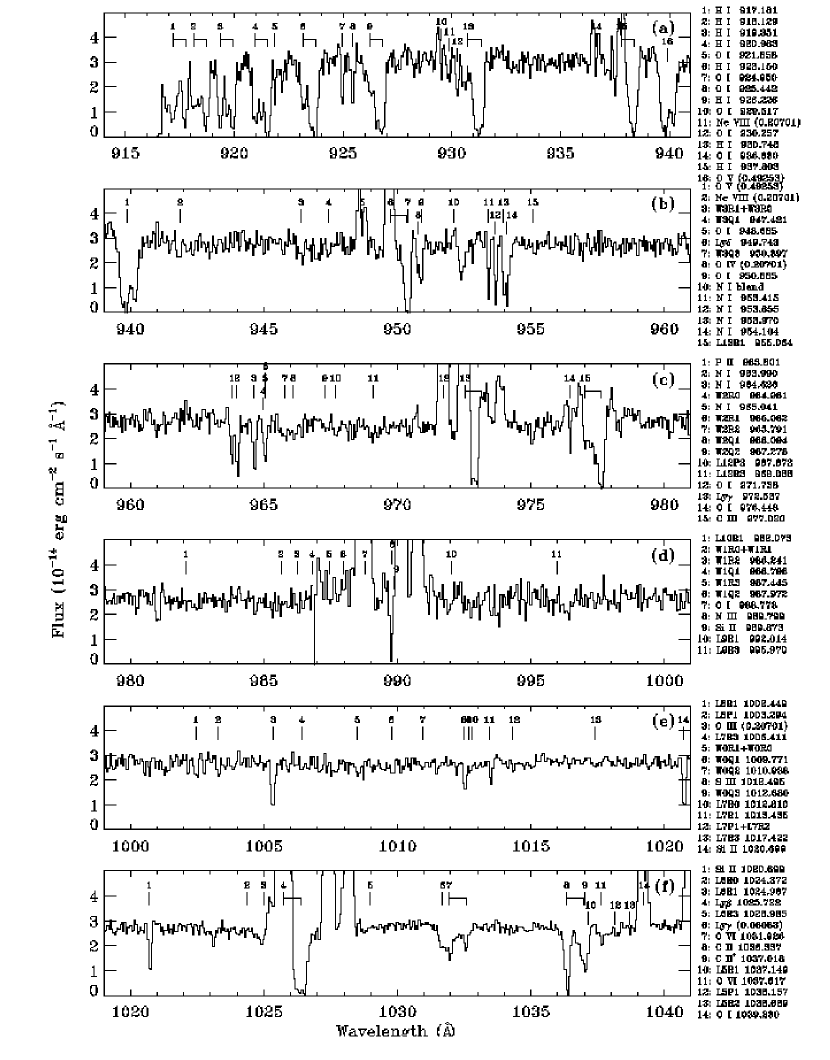
![[Uncaptioned image]](/html/astro-ph/0602085/assets/x3.png)
Fig. 2 — Continued.
![[Uncaptioned image]](/html/astro-ph/0602085/assets/x4.png)
Fig. 2 — Continued.
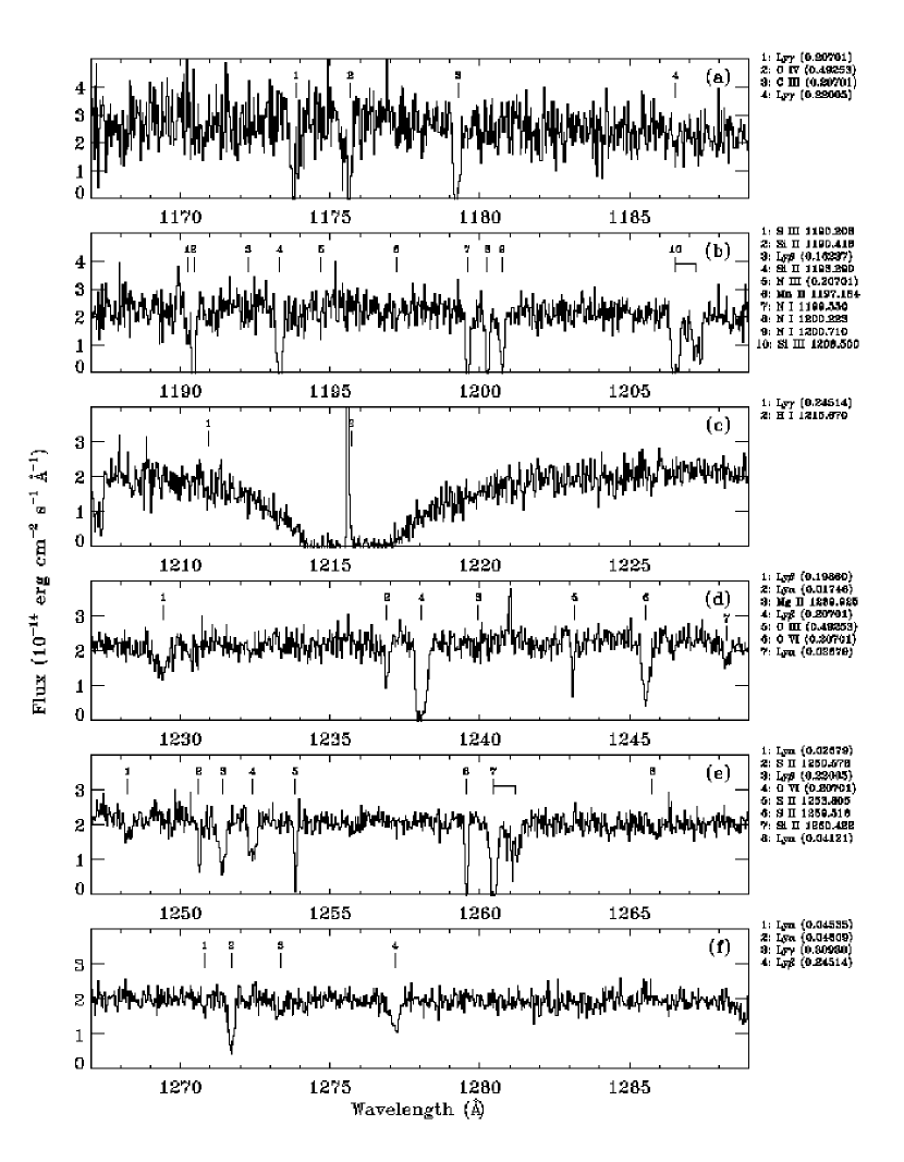
![[Uncaptioned image]](/html/astro-ph/0602085/assets/x6.png)
Fig. 3 — Continued.
![[Uncaptioned image]](/html/astro-ph/0602085/assets/x7.png)
Fig. 3 — Continued.
![[Uncaptioned image]](/html/astro-ph/0602085/assets/x8.png)
Fig. 3 — Continued.
![[Uncaptioned image]](/html/astro-ph/0602085/assets/x9.png)
Fig. 3 — Continued.
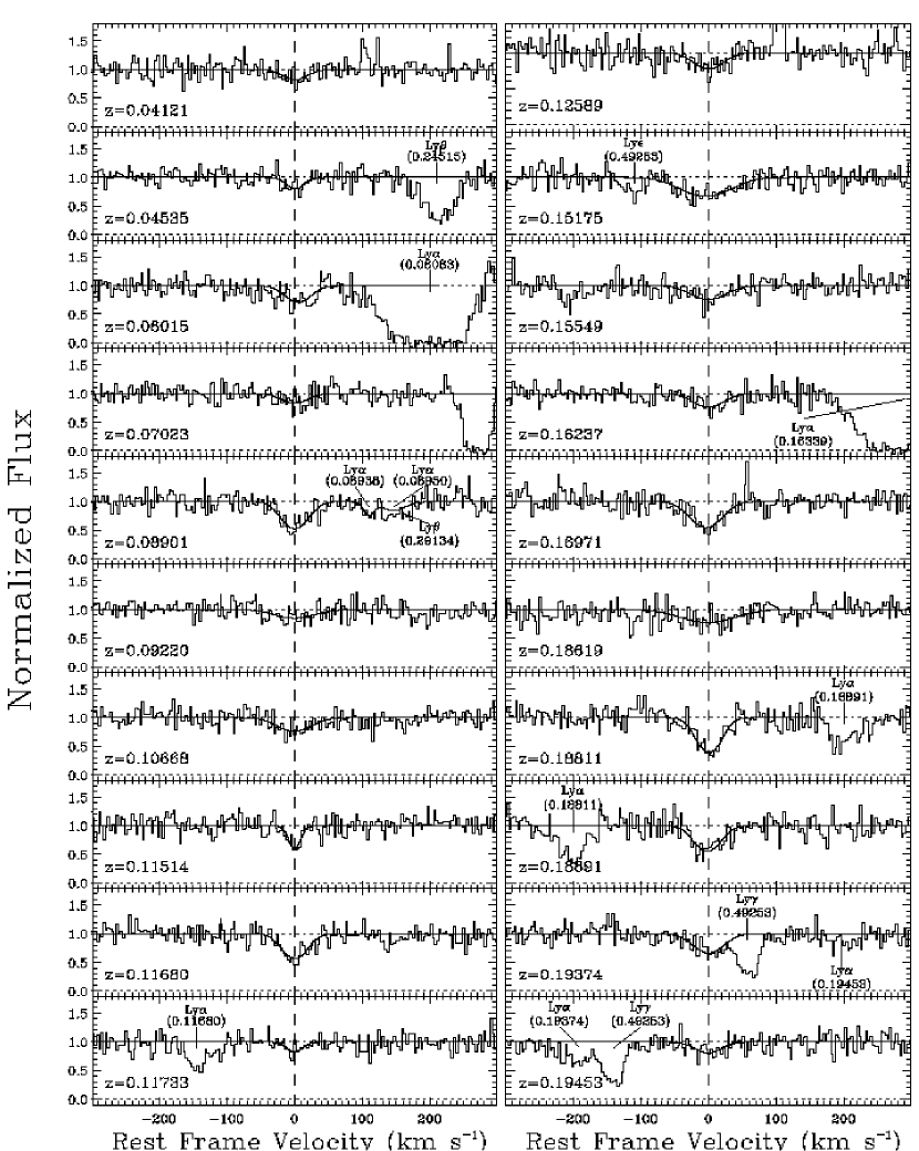
![[Uncaptioned image]](/html/astro-ph/0602085/assets/x11.png)
Fig. 4 — Continued.