Surface temperature and synthetic spectral energy distributions for rotationally deformed stars

Abstract

Extreme deformation of a stellar surface, such as that produced by rapid rotation, causes the surface temperature and gravity to vary significantly with latitude. Thus, the spectral energy distribution (SED) of a non-spherical star could differ significantly from the SED of a spherical star with the same average temperature and luminosity. Calculation of the SED of a deformed star is often approximated as a composite of several spectra, each produced by a plane parallel model of given effective temperature and gravity. The weighting of these spectra over the stellar surface, and hence the inferred effective temperature and luminosity, will be dependent on the inclination of the rotation axis of the star with respect to the observer, as well as the temperature and gravity distribution on the stellar surface. Here we calculate the surface conditions of rapidly rotating stars with a 2D stellar structure and evolution code and compare the effective temperature distribution to that predicted by von Zeipel’s law.

We calculate the composite spectrum for a deformed star by interpolating within a grid of intensity spectra of plane parallel model atmospheres and integrating over the surface of the star. This allows us to examine the SED for effects of inclination and degree of deformation based on the 2D models. Using this method, we find that the deduced variation of effective temperature with inclination can be as much as 3000 K for an early B star, depending on the details of the underlying model.

As a test case for our models, we examine the rapidly rotating star Achernar ($\alpha$ Eri, HD10144). Recent interferometric observations have determined the star to be quite oblate. Combined with the ultraviolet SED measured by the OAO-2 satellite, we are able to make direct comparisons with observations.

1 Introduction

Despite much effort, the structure and evolution of rapidly rotating stars remains one of the major problems in stellar theory for a number of theoretical and observational reasons. One significant issue is the translation of observational measurements (e.g., flux) into quantities that are related to the structure of the star, such as effective temperature and surface gravity. This translation is a comparatively simple task for spherically symmetric stars, for which the effective temperature and gravity are unique and their relationship with luminosity is well defined, but becomes more difficult for rotating stars, where both the effective temperature and gravity vary over the surface of the star. According to von Zeipel’s law (von Zeipel, 1924), the local radiative flux is proportional to the local effective gravity, which is the sum of the force of gravity and the centrifugal force, so T_eff $\propto$ g${}^{1/4}_{eff}$. This means the spectrum of a rapidly rotating star is often treated as a composite of several spectra, each at a specific effective temperature and gravity. Because the observed composite spectrum will vary with inclination, the values derived from observations will also depend on the inclination of the rotation axis with respect to the observer, something that is not known a priori.

A corollary of this law is that the relationship between the luminosity and an observed bolometric magnitude also depends on the inclination, as the amount of energy radiated from the stellar surface also varies with latitude. Thus, even something as relatively straightforward as assigning a star’s location in the HR diagram is not simple for rotating stars, as the location would not be a point but a curve with inclination as the free parameter. The length and shape of the curve would depend on the amount of surface rotation and perhaps the angular momentum distribution. The inclination determines where on the curve the observer would place the star. This effect has been well studied (Collins, 1966; Hardorp & Strittmatter, 1968; Maeder & Peytremann, 1970). These previous studies were done using spherical, uniformly rotating structural models. The distortion of the surface was described using a Roche potential and the surface variation in temperature followed von Zeipel’s (1924) gravity darkening law, with the total luminosity obeying an equation of the form L($\omega$) = L(0)f($\omega$), where $\omega$ is the fraction of critical rotation ($\Omega$/$\Omega_{crit}$). Differential rotation has been studied by Collins & Smith (1985), using a cylindrical rotation law applied to A stars. The interiors of these stars were modeled as for a 1D stellar model with three correction factors applied to account for the differential rotation. They applied these models to produce synthetic photometric observations of groups of stars. In agreement with previous studies, they find that rotation shifts a star’s location in the HR diagram, and differential rotation results in a larger shift. In this paper, we take these models one step further, applying a fully implicit 2D stellar evolution code, described in §2.1, with arbitrary rotation laws to produce our interior models. These 2D evolution simulations allow us to assess how realistic von Zeipel’s law is in several situations. This will be examined in more detail in section §3.

The observed spectral energy distribution (SED) can be found from the weighted sum of the radiative intensities emitted in the direction of the observer, integrated over the surface of the star. In principle, the SED contains information about the angular variation of the quantities which influence the radiation field. In this paper, we examine what information, if any, can be determined about the angular momentum distribution, and hence the structure, based on the SED of a star. We chose here to work with the SED rather than individual lines, as was done by Collins (1974) and Collins & Sonneborn (1979) because we hoped to be able to employ this method as a general technique over a wide range of stars. We also hoped to avoid dependence on the properties of any particular set of lines.

There are three numerical modeling components in this process. The first is the calculation of fully 2-D stellar evolution sequences with rotation (Deupree, 1990, 1995, 1998) to obtain the effective temperatures and effective surface gravities as functions of latitude for any point in a stellar evolution sequence. Here the effective temperature is defined as the black body temperature required to produce the local surface flux, and the effective gravity is the component of the centrifugal force and the gradient of the gravitational potential in the direction of the normal to the local surface (i.e., the local vertical). These two quantities are required as input parameters to the stellar atmosphere calculations. We assume that we can model the atmosphere at any given location on the surface as a plane parallel atmosphere with this local effective temperature and effective gravity. This approximation is good if the horizontal photon mean free path is very small compared to the horizontal distance over which there are significant structural changes along the stellar surface. The region where this approximation is least reliable is near the equator, where the effective gravity is smallest and the horizontal structural gradients the largest. This error is somewhat balanced by the fact that the equatorial region has the lowest effective temperature, so it contributes less to the observed flux except at inclinations of nearly ninety degrees.

The second modeling component is the calculation of a grid of model atmospheres that cover the range of effective temperatures and effective gravities required. For this we use the PHOENIX model atmosphere code (Hauschildt & Baron, 1999). These models are used to calculate the emergent intensities as a function of angle from the vertical, which will be integrated to obtain the observed flux. The main advantage to this code is the ability to model many of the important lines in non-local thermodynamic equilibrium (NLTE), while most previous studies (e. g. Maeder & Peytremann (1970)) used only LTE calculations.

The third modeling component is the numerical integration of these intensities to obtain the observed flux. The procedure used is very similar to that described in Cassinelli (1987); Linnell & Hubeny (1994); Townsend et al.  (2004). The surface of the star is divided into a mesh in longitude and latitude. For a given inclination the direction to the observer can be calculated at any location on the surface and the appropriate intensity selected from the input supplied by the model atmosphere code. This will be multiplied by the local surface area element and the cosine of the angle between the local surface normal and the direction to the observer. The sum of the intensities produced by all the mesh zones gives the spectral energy distribution of the star at a given inclination. Before integration, the intensities are convolved to match the profile of the OAO-2 spectrometers. This profile covers too large a wavelength range (10-20 Å) for Doppler shifts to be noticeable. For this reason, the Doppler shift has been neglected in this integration.

We chose this study because of the recent work of Domiciano de Souza et al.  (2003), showing that the sometime Be star $\alpha$ Eri (Achernar, HD10144) is highly oblate based on optical interferometric observations, with an axial ratio a/b = 1.56 $\pm$ 0.05. This oblateness, defined by the axial ratio, is determined by fitting an ellipse to a uniform disk model. The star is known to be relatively rapidly rotating, with vsini = 225 km s^-1 (Slettebak, 1982), but there was no indication from this or any other observations that the star was as oblate as indicated by the observations of Domiciano de Souza et al.  (2003). We were interested to see if there were indications of the degree of deformation in other available data. If so, we might be able to use these other indications to be able to determine how prevalent highly oblate stars might be, particularly for stars inaccessible by interferometric observations. The ultraviolet flux distribution for $\alpha$ Eri has been measured by the OAO-2 satellite (Code & Meade, 1979), giving us the effective temperature and luminosity of the star, as well as a SED for comparison with our models. All of these observations give us most of the information we need about the surface properties to model the star.

In the next section we present a more detailed description of the three numerical components. We discuss the surface results of the stellar evolution calculations and compare them to von Zeipel’s law in §3. In §4 we discuss the effect of various parameters on the model atmospheres as well as what was adopted and why. The synthetic SEDs produced are discussed in §5, and our conclusions are presented in §6.

2 The Codes

We wish to examine the characteristics of two rotating models with very different structure but with nearly the same horizontal average effective temperature and luminosity. Three codes are required to generate simulated SEDs for these models: the 2D stellar evolution code to provide the variation in surface values, the stellar atmosphere code to generate the single temperature SEDs and the code to integrate individual SEDs over the stellar surface. The interior and surface results alone are used to determine constraints on the applicability of von Zeipel’s law. We describe the properties of the three codes in turn.

2.1 2-D Stellar Evolution: ROTORC

The surface variation of T_eff and g_eff used to determine the size of the required grid of model atmospheres is taken from stellar evolution sequences computed with the 2.5D finite difference stellar evolution and hydrodynamics code, ROTORC (Deupree, 1990, 1995, 1998). The half dimension means that there is an equation for the azimuthal component of the momentum, but that the model is constrained to be azimuthally symmetric. Thus, the equations to be solved are the time dependent conservation laws for mass, three components of momentum, energy and hydrogen abundance, as well as Poisson’s equation. The independent variables of the code are the fractional surface equatorial radius and the spherical polar coordinate, $\theta$. The primary dependent variables are the density, temperature, three velocity components, hydrogen mass fraction and gravitational potential. The calculations are performed in the inertial frame, so the azimuthal momentum equation in principle allows the rotational velocity profile inside the star to be evolved without forcing it to be uniform or even conservative. The code was developed in this way so it can be used to perform implicit hydrodynamic simulations, albeit in 2D, to determine any hydrodynamic or secular redistribution of angular momentum. All models calculated here included core overshooting of 0.38 of the pressure e-folding distance at the convective core boundary, based on the 2D hydrodynamic simulations of Deupree (2000, 2001). The radiative opacities and equation of state are calculated from the OPAL tables (Rogers et al. , 1996).

The Zero-Age Main Sequence (ZAMS) models are calculated by specifying the rotational velocities as a function of the fractional radius and spherical polar coordinate $\theta$ and then solving for the gravitational potential, density and temperature distributions inside the star. Stellar evolution is performed in the usual way with two exceptions. Firstly, there are three components to the momentum equation and secondly, the time dependent composition equations are solved simultaneously in the implicit Henyey solution instead of explicitly outside it. The evolution sequences presented here have been calculated with local conservation of angular momentum throughout the evolution. Until the very end of the main sequence, the angular momentum distributions calculated by forcing the convective core to rotate uniformly and forcing angular momentum to be conserved locally are nearly the same because the structure of the convective core does not change much during this early evolution. We have imposed equatorial symmetry for better angular resolution with our angular zoning.

The features of primary interest here relate to the determination of the physical conditions at the surface of the stellar model. The stellar surface has traditionally been treated somewhat cavalierly in stellar structure and evolution codes, and ROTORC is no exception. For example, the radiative flux in the energy conservation equation is calculated using the 2D diffusion equation, even in the optically thin regions. At the surface, we set the flux to be equal to 2$\sigma$T${}_{surf}^{4}$, where T_surf is the temperature in the radial zone that defines the surface at each latitude (see §3 for discussion). In addition to the usual crude surface conditions, spherical diversion makes the angular zoning near the surface quite coarse, so the surface is poorly resolved in the angular coordinate, although the surface outline is not unreasonable. Some criterion must be stipulated to define the surface as a function of angle, and we have chosen to make the surface an approximate equipotential. The surface is an equipotential for conservative rotation laws, and is not unreasonable in general except when the evolutionary phase is so rapid that the stellar surface might not be able to adjust to the equipotential configuration. We take the total potential, $\Psi$, to be given in terms of the gravitational potential, $\Phi$, and the rotational ‘potential’ by

$$\Psi=\Phi-\frac{1}{2}v^{2}_{\phi}$$ (1)

The gravitational potential is determined by evaluation of the gravitational potential exterior to the stellar surface as a surface boundary condition and solving Poisson’s equation throughout the entire 2D mesh. Our models assume the second term of Eqn. 1 is a potential, but only at the model surface. This assumption will not necessarily be true for arbitrary rotation laws. The evaluation of the surface gravitational potential is included in the Jacobian generated by the Henyey perturbation technique as the appropriately weighted integral over the mass distribution. For oblate spheroids, the surface value of $\Psi$ is chosen as that value at the equator. The fractional radius of the surface at each angle is chosen as the fractional radius of the radial zone closest to the surface value of $\Psi$. Because the location of the surface is slightly quantized by the radial zoning in this way (i.e., the surface radius assumed is not quite the radius at the location of the desired value of the total potential), the value of the effective temperature may be slightly in error. The error may amount to $\sim$ 200K in rapidly rotating models. One result of this approach is that ROTORC deals only with the potential and calculates its derivatives as needed in the radial and latitudinal directions and therefore we need to solve for the direction of the surface normal at each angle in our subsequent calculations.

A key result of these 2D simulations is that we obtain values of the effective temperature, surface radius, gravitational potential, and ‘total’ potential (as defined by Eqn. 1) as a function of colatitude. This is something that 1D evolution codes, even those which include some of the effects of rotation (e.g., Pinsonneault et al.  (1989); Maeder & Meynet (2000)), do not provide except under very special circumstances. These quantities can be provided by the self consistent field method (Ostriker & Mark, 1968) calculations of Jackson et al.  (2005), but their code is currently only a stellar structure, not a stellar evolution, code, and their models to date are only ZAMS models. This variation in surface quantities is required to generate the model atmospheres described in §2.2.

2.2 Synthetic Atmospheres: PHOENIX

To generate our model atmospheres, we use the non-LTE atmosphere code PHOENIX. PHOENIX makes use of a fast and accurate Operator Splitting/Accelerated Lambda Iteration (OS/ALI) scheme to solve self-consistently the radiative transfer equation and the NLTE statistical equilibrium (SE) rate equations for many species and overlapping transitions (Hauschildt & Baron, 1999) in a stellar atmosphere. Short et al.  (1999) have greatly increased the number of species and ionization stages treated in SE by PHOENIX. At least the lowest two stages of 24 elements, including the lowest six ionization stages of the 20 most important elements, including Fe and four other Fe -group elements, are now treated in NLTE. Short et al.  (1999) contains details of the sources of atomic data and the formulae for various atomic processes.

Table 1: Species treated in Non-Local Thermodynamic Equilibrium (NLTE) in the NLTE_Light and NLTE_Fe models. Each ionization stage is labeled with the number of energy levels and bound-bound transitions included in the statistical equilibrium rate equations. Note that this table shows only a sub-set of the total number of species that are currently treatable in statistical equilibrium by PHOENIX.

Element	Model	Ionization Stage
		I	II	III	IV
H	NLTELight, NLTEFe	80/3160	$\cdots$	$\cdots$	$\cdots$
He	NLTELight, NLTEFe	19/37	10/45	$\cdots$	$\cdots$
Li	NLTELight, NLTEFe	57/333	55/124	$\cdots$	$\cdots$
C	NLTELight, NLTEFe	228/1387	85/336	79/365	$\cdots$
N	NLTELight, NLTEFe	252/2313	152/1110	87/266	$\cdots$
O	NLTELight, NLTEFe	36/66	171/1304	137/765	$\cdots$
Ne	NLTELight, NLTEFe	26/37	$\cdots$	$\cdots$	$\cdots$
Na	NLTELight, NLTEFe	53/142	35/171	$\cdots$	$\cdots$
Mg	NLTELight, NLTEFe	273/835	72/340	91/656	$\cdots$
Al	NLTELight, NLTEFe	111/250	188/1674	58/297	31/142
Si	NLTELight, NLTEFe	329/1871	93/436	155/1027	52/292
P	NLTELight, NLTEFe	229/903	89/760	51/145	50/174
S	NLTELight, NLTEFe	146/439	84/444	41/170	28/50
K	NLTELight, NLTEFe	73/210	22/66	38/178	$\cdots$
Ca	NLTELight, NLTEFe	194/1029	87/455	150/1661	$\cdots$
Fe	NLTEFe	494/6903	617/13675	566/9721	243/2592

Table 2: Levels of modeling realism.

Degree of NLTE	Model designation
None	LTE
Light metals only (H-Ca)	NLTELight
Light metals & Fe	NLTEFe

Table 1 shows which species have been treated in NLTE in the modeling presented here, and how many E levels and $b-b$ (bound-bound) transitions are included in SE for each species. E is defined as the energy of the state with respect to the ground state of that ionization stage. Table 2 explains which elements are included in the degrees of realism modeled. For the species treated in NLTE, we use the factor $gf$, where $g$ is the statistical weight of the lower level and $f$ is the oscillator strength of the transition. This factor is read in from the line lists used by PHOENIX. Only levels connected by transitions of $\log gf$ value greater than -3 (designated primary transitions) are included directly in the SE rate equations. All other transitions of that species (designated secondary transitions) are calculated with occupation numbers set equal to the Boltzmann distribution value with excitation temperature equal to the local kinetic temperature, multiplied by the ground state NLTE departure coefficient for the next higher ionization stage. We have only included in the NLTE treatment those ionization stages that are non-negligibly populated at some depth in the star’s atmosphere. As a result, we only include the first one to four ionization stages for most elements. Additionally, tens of millions of transitions are included with the approximate treatment of LTE.

NLTE effects can depend sensitively on the adopted values of atomic parameters that affect the rate of collisional and radiative processes. Atomic data for the energy levels and b-b transitions have been taken from Kurucz (1994) and Kurucz & Bell (1995). We have used the resonance-averaged Opacity Project (Seaton et al., 1994) data of Bautista et al.  (1998) for the ground-state photo-ionization cross sections of Li I- II, C I- IV, N I- VI, O I- VI, Ne I, Na I- VI, Al I- VI, Si I- VI, S I- VI, Ca I- VII, and Fe I- VI. For the ground states of all stages of P and Ti and for the excited states of all species, we have used the cross sectional data previously incorporated into PHOENIX, which are from Reilman & Manson (1979) or those compiled by Mathisen (1984). We account for coupling among all bound levels by electronic collisions using cross sections calculated with the formula of Allen (1973). We do not use the formula of Van Regemorter (1962) for pairs of levels that are connected by a permitted radiative transition because we have found that doing so leads to rates for transitions within one species that are very discrepant with each other, and this leads to spurious results. The cross sections of ionizing collisions with electrons are calculated with the formula of Drawin (1961).

For our models, we calculated intensity grids covering the region 1000 Å to 4000 Å with $\Delta\lambda$ = 0.02 Å, giving a resolution of R = $\lambda/\Delta\lambda$ = 150000.

2.3 The Atmospheric Integrator

Once we have the individual model atmospheres, we must produce an integrated flux spectrum for a model with non-uniform surface parameters. The intensity grid results from the NLTE model atmospheres are then convolved with the instrumental profile of the OAO-2 satellite (Code & Meade, 1979). Each spectrometer has a response function covering about 40 Å, so this convolution smoothes over the individual lines. For this reason, we bin the convolved intensity files to 10 Å resolution. At this resolution, the individual lines are not visible, and the bins are large enough that the effects of the Doppler shift are not significant.

The input to this code comes from stellar evolution models generated by ROTORC. We have evolved two specific models to match the approximate observed temperature and luminosity of Achernar, but with differing degrees of oblateness. From these models, we were able to generate effective temperatures and gravities as a function of latitude. These values determined the range of the atmospheric grid produced by PHOENIX. We used a grid with temperature range of 11000 to 25000K with 2000K spacing and a range in log g of 2.3 to 3.7, with spacing of 0.2. This range of temperatures is required to produce synthetic spectra of our models of Achernar.

For each wavelength, we wish to evaluate the integral

$$F_{\lambda}=\int_{\theta}\int_{\phi}\frac{I_{\lambda}(\xi(\theta,\phi))}{d^{2}}dA_{proj}$$ (2)

where $\theta$ is the colatitudinal coordinate, $\phi$ is the longitudinal coordinate, $\xi(\theta,\phi)$ is the angle between the local surface normal and the line of site to the observer, d is the distance to the object, dA_proj is the projected surface area element as seen from the direction of the observer, I_λ is the intensity at a given wavelength and F_λ is the flux at a given wavelength.

To do this integration, the surface parameters are read in from the output of ROTORC. The surface of the star is then divided into a mesh, typically 200 $\theta$ zones and 400 $\phi$ zones. For each zone, the effective temperature and surface gravity are determined from the ROTORC model. The atmospheric integration code reads in the appropriate intensities from a grid of models in T and log g produced by PHOENIX and performs linear interpolation over log T and log g to determine the intensity produced by each grid zone.

Next, the angle between the local surface normal and the line of sight to the observer ($\xi$) is determined as follows. The model is axisymmetric, so the observer can be assumed to be directly above the prime meridian ($\phi$ = 0) of the star with no loss of generality. This gives the vector coordinates from the prime meridian towards the observer of $\delta$x = sini, $\delta$y = 0 and $\delta$z = cosi.

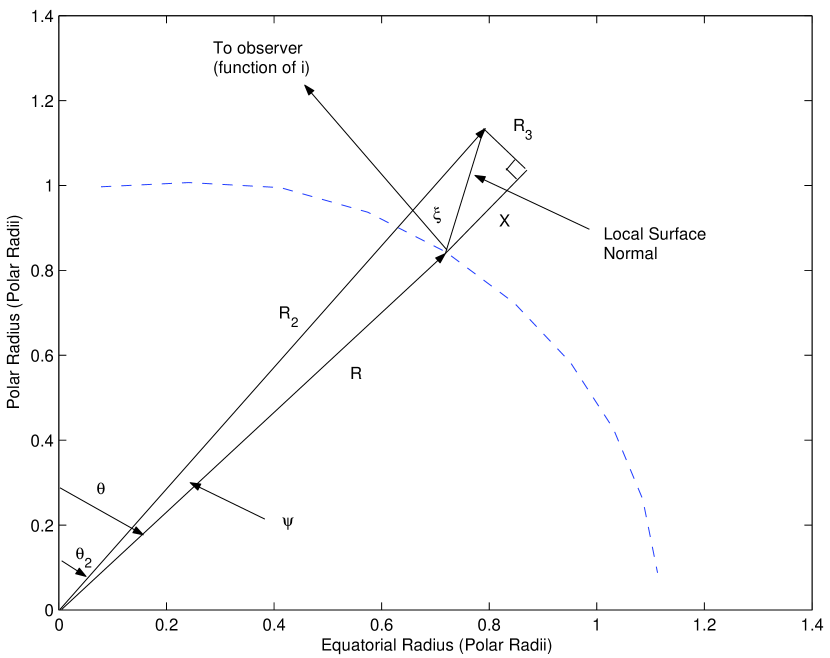
Figure 1: Schematic diagram of the geometry used to determine the vector perpendicular to the surface. The distance from the model center to the surface at the location of interest is R. This vector is extended by an arbitrary length X. R₃ is perpendicular to X and is bounded by the vector X and the vector perpendicular to the surface. The vector R₂ runs from the model center to the intersection of R₃ with the surface normal. The direction of the surface normal is given by the difference between vectors R₂ and R. The dashed line shows a sample surface geometry.

To find the surface normal, we refer to Fig. 1. Starting with the radius at a given point on the model surface, R, we extend this vector an arbitrary distance X. Next, we extend the surface normal until it meets a vector R₃, perpendicular to X. The intersection of R₃ and the surface normal occurs a distance R₂ from the center of the model. The difference between the two vectors R₂ and R is in the direction normal to the surface. If R has a polar angle $\theta$ and R₂ has a polar angle $\theta$₂, then

$$\theta_{2}=\theta-\psi$$ (3)

where $\psi$ is positive in the northern hemisphere and negative in the southern hemisphere as a result of the oblate shape of the model. The angle, $\Lambda$, between the radial vector (X) and the surface normal can be approximated by

$$tan(\Lambda)\approx\frac{\delta R(\theta)}{R\delta\theta}$$ (4)

where $\delta$R is the the variation of the surface radius over an angle $\delta\theta$.

The vector normal to the surface can be defined by the spherical coordinates (R,$\theta$,$\phi$) and (R₂,$\theta$₂,$\phi$), of which R, $\theta$,$\phi$ and $\Lambda$ are known and X is assumed. From these, we can calculate

$$R_{3}=Xtan\Lambda$$ (5)

$$R_{2}^{2}=(R+X)^{2}+R_{3}^{2}$$ (6)

$$\psi=arcsin(\frac{R_{3}}{R_{2}})$$ (7)

Given these quantities we can perform the dot product of the vector R₂ -R with the line of sign vector to find cos$\xi$. There are other ways by which the normal could be calculated. One of these would be to use the vector sum of the gravitational and centrifugal forces, as this sum is normal to the equipotential surface. This would then be interpolated between the centers of the angular zones. We decided to use the equipotential as defined by Eqn. 1 because this is what the 2D code uses to determine the surface location. Given the collection of approximations made in the calculation, we do not regard the uncertainties in this aspect of the calculation as sufficiently significant to investigate different methods.

Equations 4 to 7 allow us to calculate the direction cosine between the surface normal and the vector pointing towards the observer, $\xi$. By definition the surface is not visible to the observer if cos$\xi$ $<$ 0.

Once cos$\xi$ has been determined, an interpolation over the angles in the intensity files is performed. This gives the contribution to the total flux per wavelength from each grid zone. This total flux is then weighted according to the projected surface area for each mesh zone

$$dA_{proj}=R(\theta)^{2}sin\theta cos\xi\sqrt{1+\Big{(}\frac{dR}{Rd\theta}\Big{)}^{2}}d\theta d\phi$$ (8)

The process is then repeated for each wavelength. For these models, we calculated the flux for every 10 Å for wavelengths covered by the OAO-2 spectrometers, 1160 to 3600 Å. This allows for direct comparison with the UV spectrum taken by the OAO-2 satellite. However, this is not a limitation on the code, and any wavelength range or spacing could be used.

To ensure that the integrator worked correctly, we compared the final flux spectrum for a uniform sphere produced by PHOENIX and by our atmospheric integrator. PHOENIX performs the integration by adding up the contributions of a series of concentric annuli (Mihalas, 1978, pp 11-12), while our integrator uses a mesh in $\theta$ and $\phi$. This method produces a finer mesh in the polar regions than near the equator. The two flux spectra are very similar overall, although there are some slight variations. These variations are thought to be due to slight numerical differences in the methods of integration. Another difference between these two models is the order of operations. In our model, we convolve the 0.02 Å spaced intensity grid and then integrate the product. In the PHOENIX model, the SED is calculated at 0.02 Å and then convolved. We checked that these two operations commute by integrating a small section of the intensity grid at a resolution of 0.02 Å and then comparing it to the PHOENIX flux spectrum. The two unconvolved spectra differ by about 0.8% over a region spanning 150 Å.

We also tested the spacing of our grid. Initially, our models were spaced at intervals of 0.2 in logg and 2000 K in temperature. In general, we found the difference between successive gravities was very small, so we concluded the resolution in logg was sufficient. We used our integrator to produce a SED for a model at 12000 K based on intensity files at 11000 and 13000 K. Next, we compared this to a SED based on the the intensity files at 12000 K. To estimate how accurate the interpolation was, we took the ratio of the two 12000 K models. The fourth root of this ratio gave us an estimate of the ratio of the temperatures corresponding to these fluxes. On average, the ratio calculated was 0.98, corresponding to a 2% error in the temperature. We concluded that this amount of error was acceptable, and hence our temperature spacing of 2000 K was sufficient.

3 Comparison of Evolutionary Surface Results with von Zeipel’s Law

A general way of exploring the effective temperature variation on the surface of a rotating star under specific assumptions was outlined by von Zeipel (1924). If the centrifugal acceleration is conservative, it can be written as the gradient of a potential. This means that the gradient of the pressure is given by the density times the gradient of the sum of this potential and the gravitational potential. Thus, the pressure is constant on the equipotential surface, and the density must be as well. If the equation of state is a function of the density, temperature, and composition, then the temperature will also be constant on the equipotential surface if the composition is uniform. If the energy transport is by radiation and the diffusion approximation may be used for the radiative flux, then the energy flow must be perpendicular to the surfaces of constant temperature, i.e., perpendicular to the equipotential surfaces. This flux can be written in terms of the gradient of the total potential, which is just the effective gravity. At the surface this flux is proportional to the fourth power of the effective temperature, so we have

$$T_{eff}\propto g_{eff}^{0.25}$$ (9)

Here we wish to compare the results of our evolution calculation surfaces with those based on this simple model. There are several possible sources of disagreement. One feature that the simple model fails to treat is the coupling of the effective temperature to the surface temperature structure in any way. This surface temperature structure will not alter the temperature structure of the model much, except near the surface, but it could play a role in situations near critical rotation, where the von Zeipel model predicts that equatorial effective temperature vanish as the effective potential goes to zero, or in other situations in which there is significant variation in effective temperature between the pole and equator.

To make this comparison we will examine four models from two evolutionary sequences. Two of the models are ZAMS models, one for a uniformly rotating model near critical rotation, and the other for a model with significant differential rotation. We use the parameter $\eta$

$$\eta=\frac{\Omega^{2}R_{e}^{3}(\Omega)}{GM},$$ (10)

the ratio of the centrifugal and gravitational forces at the equator. At critical rotation, this parameter should have the value 1. The uniform rotation ZAMS models has a surface equatorial velocity of 495 km s^-1 and $\eta$ = 0.86. The ratio of polar to equatorial radius is 0.70. The differentially rotating model had a surface equatorial velocity of 410km s^-1 on the ZAMS, which gives $\eta$ = 0.56. The ratio of the polar to equatorial radius is 0.78. Each of these ZAMS models is then evolved through core hydrogen burning and a model with the average luminosity and effective temperature close to those observed for Achernar chosen. These two evolved models will be compared with the observed SED of Achernar as well as each other. Because of the effects of rotation on the surface properties, different rotation laws require different masses to reproduce the same average surface temperature and total luminosity. As the rotation increases, the model moves down and to the right in the HR digram when plotted using its “average” surface quantities. To compensate for this effect, the mass must be increased to raise the average luminosity. Increasing the internal angular momentum for a given surface velocity has the same effect. Our models are not as oblate as those described in Jackson et al.  (2004) because we are not yet able to model such extreme angular momentum distributions. The 2D code currently expects the equator to have the largest radius, and for very high angular momentum models, such as the distributions described in Jackson et al.  (2004), this is not the case.

These evolutionary sequences locally conserve angular momentum. This is different from the usual assumption of forcing uniform rotation in the convective core. However, the two approaches give very nearly the same result until the very end of core hydrogen burning is reached, because the density structure in the core does not change significantly until that stage is reached. It should be noted that the evolved models will not have conservative rotation laws, although the departures from a law which depends only on distance from the rotation axis are slight.

The surface effective gravity is calculated in a relatively straight forward way. From the surface shape, we can determine the angle between the radial and the normal to the surface. Because we know both the radial and latitudinal variation of both the gravitational and centrifugal forces, the effective gravity follows.

First we examine the uniformly rotating case. The variation of the ROTORC gravitational potential on a sphere with radius equal to the surface equatorial radius is quite small, only about 0.1% between the pole and equator. This is not surprising because even near critical uniform rotation the inner regions do not rotate sufficiently fast to produce any significant horizontal variation in the mass distribution which would show up in the surface gravitational potential. A comparison of the effective temperatures from ROTORC and from von Zeipel’s law are shown as a function of colatitude Fig. 2. The effective temperatures calculated from von Zeipel’s law show a greater range than do those from the 2D model, being both larger at the pole and smaller at the equator. At least part of this arises from the conditions at the equator; the ROTORC surface flux there is more than four times greater than the von Zeipel model flux. This must be compensated for somewhere, as the luminosity emitted by the two models is required to be the same. As a result, the von Zeipel polar temperature and flux are higher than the ROTORC values.

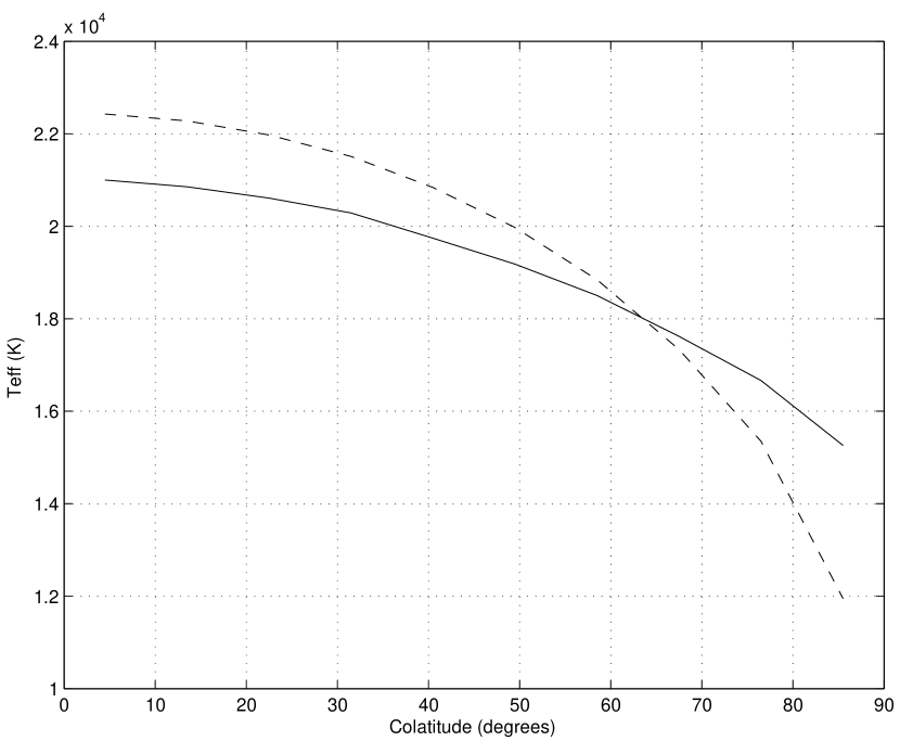
Figure 2: Comparison of the effective temperature variation for the 6.5 M_⊙ ZAMS model rotating as a solid body near critical rotation (solid) and from von Zeipel’s law (dash). von Zeipel’s law is calibrated so that the total flux radiated from the surface is the same as that for the ROTORC model. The von Zeipel equatorial flux may be too low because the effective temperature is not coupled to the temperature near the surface of the model.

We believe the source of the disagreement between our calculation and the von Zeipel model can be found in a contradiction in the von Zeipel model. The von Zeipel model argues that the temperature is constant on an equipotential surface, but the effective temperature varies significantly from the pole to the equator. This can be true only if the effective temperature is completely independent of the surface temperature structure of the star. Our models require the temperature in the last zone to be given by the surface ($\tau$ = 0) temperature of a simple grey atmosphere:

$$T(\tau)^{4}=\frac{3}{4}T_{eff}^{4}(\tau+\frac{2}{3})$$ (11)

so the surface flux is just 2$\sigma$T($\tau$=0)⁴.

To determine if this could be the source of the differences in Fig. 2, we integrated model envelopes (in the stellar structure sense) from the surface inward. A common approach is to assume values of L, T_eff, M and the composition and start with a very small density, $\rho$($\tau$ = 0), at r = R. Although a number of variations are possible, most do not matter unless the envelope is highly extended. Our integration scheme is modeled on a code Packzynski (1969) developed to produce outer boundary conditions for his stellar evolution codes, but the code has been updated to include the same physics as ROTORC. We modified the envelope integrator to decouple the effective temperature and the surface temperature by treating the surface temperature as a free parameter. We then compared the density, temperature and pressure distributions of model envelopes for a given effective temperature but with a range of surface temperatures.

As one would expect, the differences decrease with depth into the model. However, the differences only drop to about one percent at temperatures of about 6$\times$10⁵ K, which is about the variation we see along equipotential surfaces at these temperatures. This is not an ironclad argument because we have not included the centrifugal force in these envelope calculations, but it is suggestive.

The evolved model shows that these differences have been significantly reduced, as the ROTORC model is now much less oblate. The ratio of the polar to equatorial radius is now 0.81 and the rotational surface equatorial velocity has dropped to 278 km s^-1, with $\eta$ = 0.45. Note that this surface equatorial velocity is close to the value of v sini for Achernar, but the ROTORC model is much less oblate. The range of temperatures predicted by the von Zeipel model is still slightly larger, but in no location is the temperature difference between the two models greater than 350 K. The discrete zoning of the ROTORC models produces about a 200 K difference if the surface is changed by one radial zone, so this uncertainty already accounts for a sizable fraction of this temperature difference. Note that because of local conservation of angular momentum, the ROTORC rotation law is no longer conservative after the evolution, but the departures are small with no obvious consequences.

The situation for strongly differentially rotating stars raises different issues. For the rotation law, we have followed the general form of Jackson et al.  (2004):

$$\Omega=\frac{\Omega_{\circ}}{1+\alpha\varpi^{n}}$$ (12)

The exponent was chosen to be 1.4 and the constant $\Omega_{\circ}$ chosen so that the surface equatorial velocity of the ZAMS model was 430 km s^-1. The coefficient ($\alpha$) of the distance from the rotation axis ($\varpi$) is 2.0 in units where the surface equatorial value of $\varpi$ is unity. The rotation law is conservative and the model has significant differential rotation.

Fig. 3 compares the effective temperature as a function of polar angle between the calculated ROTORC model and von Zeipel’s law. The most significant difference is the higher temperature at the pole in the ROTORC model although both ROTORC and von Zeipel’s law show the same general shape in the latitudinal effective temperature dependence.

A number of calculations were undertaken to determine the origin of the differences in Fig. 3 and the sensitivity of the computed results. Both the radial and angular zoning resolution were increased appreciably, but there was no significant effect on the surface temperature latitudinal dependence. The largest effect of more refined zoning was the dropping of the variation of the density, pressure, and temperature on equipotential surfaces (calculated after the fact). In the relatively deep interior these variations were about 0.1% with the current zoning, and were reduced to about 0.03 % when the angular resolution was doubled. This amount is also about the departure of the numerical calculation of $\bigtriangledown^{2}(1/2(v_{\phi}^{2}))$ from $2\omega^{2}$ for the uniform rotation case. The radial zoning was already quite good and the changes of the variables on equipotential surfaces was very slight. We also examined the calculation of the radiative gradient, $\bigtriangledown_{rad}$, near the convective boundary by using the actual computed pressure gradient instead of the usual stellar structure expression based on spherical symmetry. The changes in the uniformly rotating model were negligible because the rotation near the convective core boundary is so low, but for this steep differential rotation it did change the location of the convective core boundary slightly, but again had no effect on the latitudinal variations of the surface temperature. From these results and some other artificial numerical exercises we conducted, we believe the differences between the surface temperature latitudinal variations originates at or near the surface.

There are at least two surface possibilities to explain the differences. One is that, unlike the uniformly rotating case, the surface shape variations are fairly large close to the rotation axis, even though they must go to zero on the axis because of the axial symmetry. This makes the calculation of the normal to the surface somewhat uncertain and thus the contribution of the rotational potential in this direction is uncertain as well. Another is rooted in the same cause as for the uniform rotation case - the decoupling of the effective temperature from the surface temperature structure in von Zeipel’s law.

One might wonder how the envelope could produce one situation in which von Zeipel’s law shows greater variation than the 2D calculation in one case but less in the other. Part of the reason can be seen by comparing the polar and equatorial temperatures on equipotential surfaces as functions of depth into the model from the surface. In the uniform rotation case, the two temperatures started off at the surface values and progressively approached each other as the depth into the model increased. This is not true in the differential rotation case, where the significant difference in the opacity for the surface temperatures allows the two temperatures to cross on an equipotential surface on which the polar temperature is still optically thin because the opacity is appreciably lower. These two temperatures separate further as a function of depth although this eventually stops and they gradually come together again at sufficient depth in the envelope. This temperature at which the polar and equatorial temperatures come together is effectively the same for uniform and differentially rotating model.

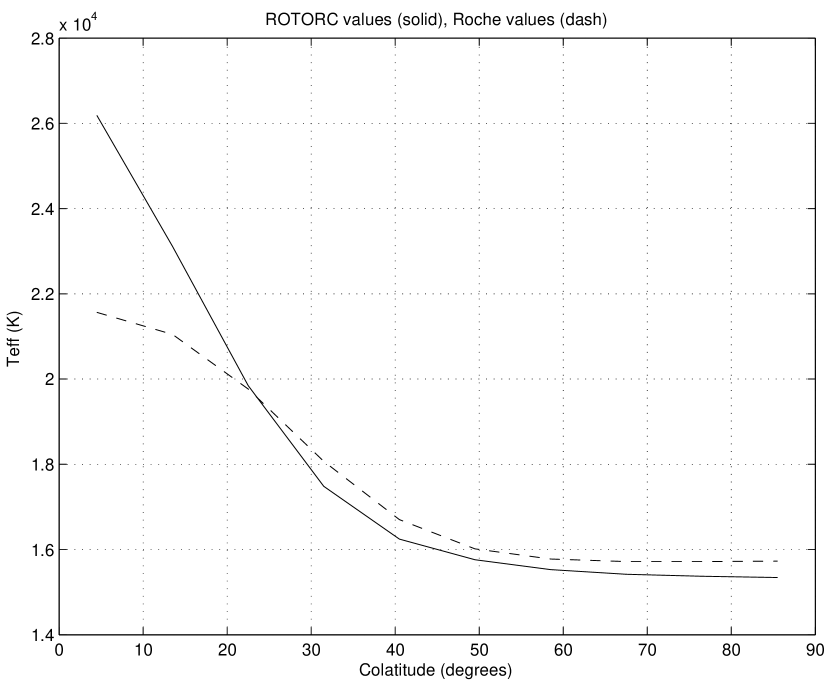
Figure 3: Comparison of the effective temperatures for the 7 M_⊙ differentially rotating ZAMS model (solid) and von Zeipel’s law (dash). The ROTORC model clearly funnels more energy toward the high latitude regions than von Zeipel’s law would predict.

4 Atmospheric Models

Before we calculate our model atmospheres we must specify the composition. Several lines of evidence weakly point to using a composition which is approximately solar. In this context a metal abundance of 0.02 is sufficiently close to the solar value of 0.0188. Recent photospheric modeling points to a much lower iron abundance, based on rather uncertain oscillator strengths (Kostik et al. , 1996). We have chosen to use the solar abundance required to reproduce the helioseismology results for a 1 M_⊙ at the solar age, around Z $\sim$ 0.018 (Antia & Basu, 2005; Bahcall et al. , 2005). The observational evidence for a metallicity approximately solar includes the fact that Achernar is close to the sun (d = 44.1 pc) (Perryman et al. , 1997) and hence its metallicity is likely close to solar. Another indication of the metallicity of Achernar comes from a study by Torres et al.  (2000) which finds some evidence for a lose association of pre-main sequence stars centered around ER Eri. Although this association consists primarily post-T Tauri stars, the age and location of Achernar is consistent with a metallicity of Z = 0.02. Finally, many studies of galactic B stars indicate their average metallicity is close to solar (Gehren et al. , 1985; Brown et al. , 1986; Lennon et al. , 1990). We have run comparisons of LTE models with Z = 0.02 and Z = 0.04. The higher metallicity models show more line blanketing, but the differences between the two SEDs are too small to have a preference of one metallicity over the other when compared to the observed SED of Achernar. Based on this admittedly weak evidence, we have performed all our calculations with Z = 0.02.

We also calculated models making various assumptions about NLTE. We have compared models in which all energy levels are populated according to LTE, models in which only the light elements are allowed to be in NLTE and models in which the light elements and Fe are assumed to be in NLTE (see Table 2). The differences among the three resulting SEDs were sufficiently large and changed the shape of the SED just enough that we felt that the models with both the light elements and Fe in NLTE were needed. The remaining discussion uses these models.

Here we shall focus on a model from each of the two stellar evolution sequences which most closely approximate the average conditions of Achernar. As one might expect from Figs. 2 and 3, the observed SED depends on the inclination of the observer to the rotation axis. This is shown in Figs. 4 and 5, which shows the observed spectrum of models inclined at 0, 30, 60 and 90 degrees. The spectra shown in Fig. 4 are based on an evolved 6.5 M_⊙ model with uniform rotation on the zero-age main sequence (ZAMS) and a surface equatorial velocity of v = 495km s^-1. This model has been evolved to a temperature and luminosity of T = 14510K, L = 3311 L_⊙, corresponding to the effective temperature and luminosity of $\alpha$ Eri (Code et al. , 1976). These observed parameters were determined without considering the effects of rotation, and so are only apparent parameters. At this point, our model has an oblateness of only a/b = 1.19. Those in Fig. 5 are based on an evolved 7.0 M_⊙ model, rotating on the ZAMS with a power law described by Eqn. 12. The ZAMS surface equatorial velocity of this model is v = 430km s^-1. The ratio of equatorial axis to polar axis is a/b = 1.32 on the ZAMS. All spectra in this section are calculated assuming a distance of 40.0 pc to Achernar, based on the OAO-2 data (Code et al. , 1976).

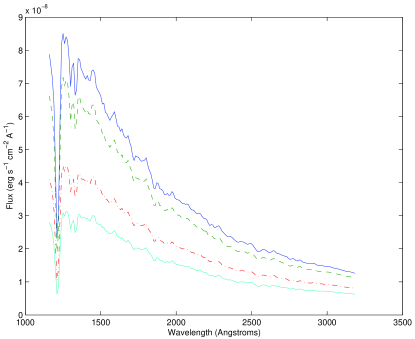
Figure 4: Synthetic flux spectra for a 6.5 M_⊙ model at inclinations of 0^∘ (top solid) 30^∘ (dashed) 60^∘ (dot dashed) and 90^∘ (lower solid).

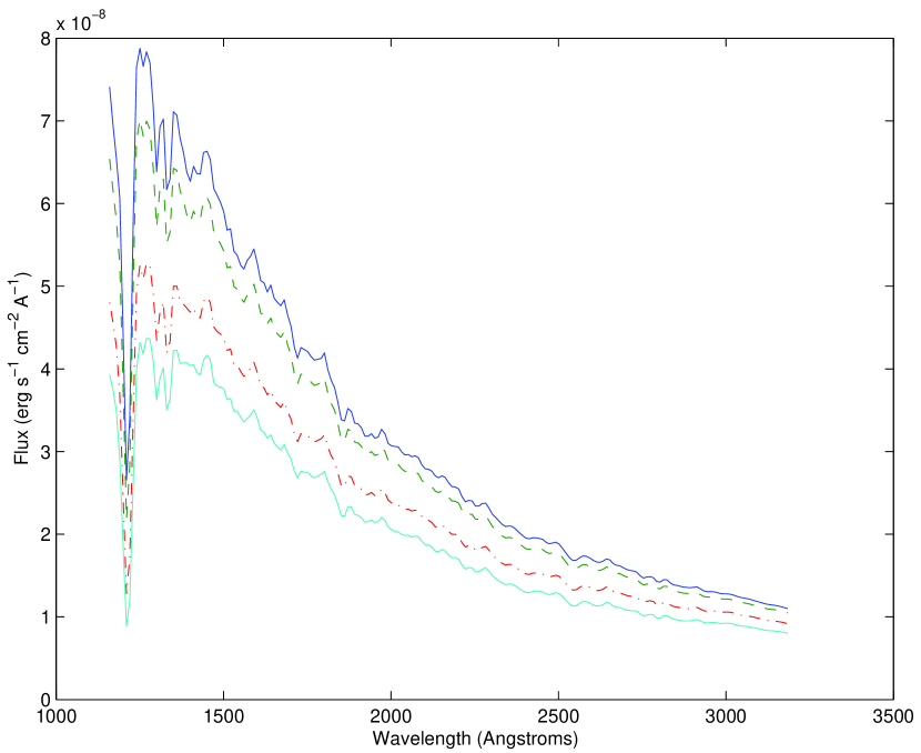
Figure 5: Synthetic flux spectra for a 7.0 M_⊙ model at inclinations of 0^∘ (top solid) 30^∘ (dashed) 60^∘ (dot dashed) and 90^∘ (lower solid).

We defined four passbands based on the variation of the spectra among the model atmosphere grid to generate color indices for evaluating the properties of these models. The four passbands are: A: 1440-1460 Å, B: 1250-1280 Å, C: 3100-3180 Å D: 1900-1940 Å. The color indices we used are A-B, A-C and A-D. As a fourth color, we also calculated a Ly $\alpha$ index, taking the ratio of the flux at the bottom of the Ly $\alpha$ line (1210 Å) to the flux at a point just redward of this line ($\sim$ 1240 Å). We calculated the color index for each one of the atmosphere models used to produce the synthetic spectra, which we then used to calibrate the color indices agains T_eff and log g. This allowed us to calculate apparent temperatures for the synthetic SEDs. This apparent temperature does not necessarily correspond to the physical temperature anywhere on the star, but gives an effective average temperature, roughly corresponding to the observed temperature of the object. As a check on these inferred temperatures, we also calculated fits to the color-temperature data for the other three color indices. The results were quite similar for all four indices, and suggest an uncertainty in these temperature estimates of $\pm$ 300 K.

Calculations were made every 10^∘ of inclination. Because the polar region of these oblate models is hotter than the equator, the more pole on the star is, the higher the apparent effective temperature of the star. In the spectra shown in Figs. 4 and 5, the inferred temperature difference between 0 and 90 degrees is between 2500 and 3000 K, depending on the details of the model. This is illustrated in Fig. 6, which shows the inferred effective temperature as a function of inclination for the two models described above.

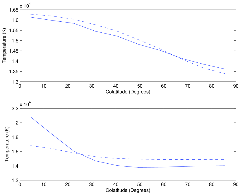
Figure 6: Top: The “observed” effective temperature (solid) as a function of inclination for the 6.5 M_⊙ model. The dashed lines shows the calculated surface temperature as a function of colatitude for the same model. Bottom: Same as for top plot, but for the 7 M_⊙ model. Both models are evolved to approximately match the observed properties of Achernar.

Clearly, for more extreme angular momentum distributions, the temperature difference between the pole and the equator is larger. The apparent effective temperatures for these models ranges between 13000K and 18000K, and the luminosity ranges are correspondingly large. The inclinations that best correspond to the ROTORC temperature of 14500K are approximately 40^∘ for the 7 M_⊙ model and 65^∘ for the 6.5 M_⊙ model. However, the inclinations required to match vsini are 90^∘ and 82^∘ respectively. This suggests that the set of information contained in the observed L, T_eff and v sini data might be able to decouple the inclination, but these limited calculations are insufficient to show either that this can be done or that the solution is unique. Work in this area has been done by Maeder & Peytremann (1970), for example, and seems to indicate that the solution is indeed not unique.

The range of possible observationally determined temperature and luminosity for a given star is illustrated in Fig. 7. The range of possible values is centered on the location in this case, as our ROTORC temperature is an average. A real observation of a single star results in a single point in the HR diagram. If the star is known to be rapidly rotating, this could result in a huge uncertainty in its intrinsic position in the HR diagram. Without knowing the physical inclination of a rapidly rotating star, there is no way to determine where on this curve the star actually lies.

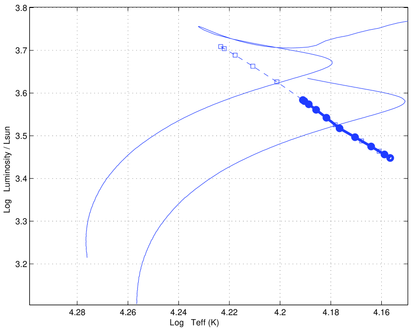
Figure 7: The possible temperature and luminosity ranges of our models as functions of inclination. The dashed line shows the values for the 7 M_⊙ model, while the solid bold line shows the values for the 6.5 M_⊙ model. The points marked show the postion for every 10^∘ of inclination (from left to right) 0^∘ to 90^∘ for the 6.5 M_⊙ ($\circ$) and 7 M_⊙ ($\square$) models respectively. The evolutionary sequences for 7 M_⊙ and 6.5 M_⊙ uniformly rotating models are shown for reference.

It remains to be determined if the SED contains sufficient information to determine the pole to equator temperature range. We compare the SEDs produced by the 6.5 and 7 M_⊙ rotating models in Fig. 8, along with the SED for Achernar, based on the OAO-2 data (Code & Meade, 1979). The properties for these three SEDs are summarized in Table 3. The inclinations of the two models were chosen to provide the best fit to each other at wavelengths greater than $\sim$ 1700 Å. The best fit for the 6.5 M_⊙ model was chosen by visually matching the red tail of the SED ($\lambda$ $>$ 2500 Å) and was found to fit best at 80^∘. We used linear interpolation to match the 7 M_⊙ model to the 6.5 M_⊙ model, and found a match at 84^∘. To match the observed vsini of Achernar, these models must be inclined at 90^∘ and 82^∘ respectively.

We find very few differences between the SEDs of the two models, and neither provides a particularly good match to the observed SED of Achernar. The two synthetic spectra give reasonably good matches throughout most of the tail region, beyond $\lambda$ $\sim$ 1700 Å. Near the peak of the SED, the 7 M_⊙ model has a slightly higher flux than the 6.5 M_⊙ model. The observed spectrum of Achernar has even more flux in this region of the spectrum. At this point in the evolution of the models, the 6.5 M_⊙ model is slightly more oblate, although the 7 M_⊙ model has a larger variation in surface temperature. This suggests that to successfully reproduce the observations would require even more extreme differentially rotating models. It may be possible to exploit differences that exist in the individual lines of these spectra (Collins, 1974; Collins & Sonneborn, 1979), but this is beyond the scope of the present work.

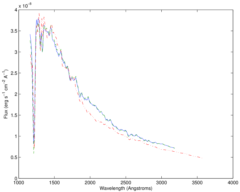
Figure 8: The SED for a 6.5 M_⊙ model (solid) inclined at 80^∘ and a 7 M_⊙ model (dashed) inclined at 84^∘. Although the structure of the two models is very different, there are only small differences in the SEDs. The 7 M_⊙ model, which has a larger surface temperature range, is slightly closer to the observed spectrum of Achernar (dot-dashed). This suggests that models with very extreme surface variations, presumably requiring extreme differential rotation, could be used to reproduce the observations.

It is possible to reach an oblateness of 1.5 with an object rotating uniformly very close to critical velocity, this does not explain the observed oblateness of Achernar. Although an object uniformly rotating at critical velocity can reach a high enough oblateness to match the observations, the resulting vsini will not match the observed value for Achernar. As the object must be viewed edge on to match the observed oblateness, i $\sim$ 90^∘. This implies that the observed vsini of 225 km s^-1 is the actual velocity of the object, yet this is clearly well below critical rotation for this type of star. As the star evolves along the main sequence, the problem worsens. There is no reason to believe the star maintains uniform rotation, and as the surface expands, the surface velocity will drop and the star will become less oblate. As Achernar appears to be an evolved main sequence star, to have the observed oblateness at the observed vsini requires differential rotation.

Table 3: Properties of models compared to the observed properties of Achernar

Model	Teff (K)	L (L⊙)	veq (km s-1)	Inclination	a/b (observed)
Achernar	14510	3311	2251	unknown	1.56
6.5 M⊙	14649	3377	223	82o	1.20
7.0 M⊙	14492	3752	208	90o	1.17

¹ Observed v sini.

Note: The observed oblateness of the models is given based on the angle of inclination required to match the observed vsini of Achernar.

5 Conclusions

We have calculated the internal structure and surface variation of models for two rapidly rotating stellar evolution sequences using the 2D stellar evolution code ROTORC. One sequence was uniformly rotating on the ZAMS, the other differentially rotating. This evolution code allows us to directly model the surface variation in effective temperature and gravity, which we can then compare with the predictions made by von Zeipel’s law.

We find our models are reasonably close to the predictions of von Zeipel’s law, although there are some pronounced differences. The difference predicted by our uniformly rotating model is largely a result of the equatorial flux. ROTORC predicts a much higher equatorial flux than the von Zeipel model, which must be compensated by higher flux at the pole to keep the total luminosity the same. We believe this difference arises as a result of an inherent contradiction in von Zeipel’s law. One of the fundamental assumptions of this model requires that the temperature be constant on equipotential surfaces. The surface is also assumed to be an equipotential surface. However, the effective temperature varies over the surface of the star. We believe this decoupling of the surface and effective temperatures gives rise to the difference between the two models. The differences are similar in form, although reduced in magnitude, when the evolved model is compared.

For differentially rotating models, the situation is quite different and the agreement with von Zeipel’s law is not as good as for the uniformly rotating models. Our models predict an appreciably higher temperature at the pole than the von Zeipel model. We have performed several calculations to investigate the source of this discrepancy, including varying the model zoning and some details of the calculations in the convective core. We found that none of these changes had any significant effect on the temperature differences, leading us to suspect that the discrepancy is produced by some aspect of our surface treatment.

Following the example of many previous studies, we have calculated the spectral energy distribution of a deformed star. However, unlike previous work, which relied on von Zeipel’s law, our SEDs are based on the surface parameters obtained directly from 2D stellar structure models. While our models are rotationally deformed, in principle this method could be used on any type of deformed star, such as a companion in a close binary. This method is also valid over any spectral range and resolution, as long as the appropriate model atmospheres and intensity grids can be produced. However, at higher resolution, Doppler effects would need to be included.

We find significant differences in the observed SED as a function of the inclination of the rotation axis to the observer. These differences could mean that the effective temperature determined by an observer may have no relation to the physically meaningful blackbody temperature of the star as a whole. By comparing the SEDs resulting from two different stellar structure models, we have found that there are a few minor differences. These are not necessarily related to the oblateness of the model, but do seem to depend on the variation in surface temperature from pole to equator. For these models, the greater this variation, the more sharply peaked the resulting UV spectrum.

We have also attempted to find a match to the spectral energy distribution of Achernar based on the OAO-2 observations Code & Meade (1979). Of the synthetic SEDs we have produced, the best matches are models inclined at 80^∘ and 84^∘, corresponding to the 6.5 and 7 M_⊙ models respectively. These inclinations also correspond quite well to the inclinations required to match the observed vsini of Achernar, 82^∘ and 90^∘ respectively. Unfortunately, our matches are far from perfect, particularly near the peak of the UV spectrum, near 1500 Å. Neither of the underlying stellar models were as oblate as the observations of Domiciano de Souza et al.  (2003) indicate Achernar to be. If the increased oblateness also corresponds to an increase in the difference in surface temperature from pole to equator, than it is possible that sufficiently differentially rotating models could reproduce the observations. We expect to produce models with higher angular momentum distribution in the near future.

References

- Allen (1973) Allen, C. W. 1973, Astrophysical Quantities (3d ed.; London: Athlone)
- Antia & Basu (2005) Antia, H.M. & Basu, S. 2005. ApJL, 620, L129
- Bahcall et al. (2005) Bahcall, J.N., Serenelli, A.M. & Basu, S. 2005. ApJL, 621, L85
- Bautista et al. (1998) Bautista, M. A., Romano, P., & Pradhan, A. K., 1998, ApJS, 118, 259
- Brown et al. (1986) Brown, P.J.F., Dufton, P.L., Lennon, D.J. & Keenan, F.P. 1986. MNRAS, 220, 1003
- Cassinelli (1987) Cassinelli, J.P. 1987. in Physics of Be stars, ed. A. Slettebak & T.P. Snow (Cambridge: Cambridge Univ. Press), 106
- Code et al. (1976) Code, A.D., Davis, J., Bless, R.C. & Hanbury Brown, R. 1976. ApJ, 203, 417
- Code & Meade (1979) Code, A.D. & Meade, M.R. 1979. ApJS, 39, 195.
- Collins (1966) Collins, G.W. 1966. ApJ, 146, 914
- Collins (1974) Collins, G.W. 1974. ApJ, 191, 157
- Collins & Sonneborn (1979) Collins, G.W. & Sonneborn, G.H. 1979. ApJ, 34, 41
- Collins & Smith (1985) Collins, G.W. & Smith, R.C. 1985. MNRAS, 213, 519
- Deupree (1990) Deupree, R.G. 1990. ApJ. 357, 175
- Deupree (1995) Deupree, R.G. 1995. ApJ, 439, 357
- Deupree (1998) Deupree, R.G. 1998. ApJ, 499, 340
- Deupree (2000) Deupree, R.G. 2000. ApJ, 543, 395
- Deupree (2001) Deupree, R.G. 2001. ApJ, 552, 268
- Domiciano de Souza et al. (2003) Domiciano de Souza, A., Kervella, P., Jankov, S., Abe, L., Vakili, F., di Folco, E., & Paresce, F. 2003. A&A, 407, L47
- Drawin (1961) Drawin, H. W., 1961, Z. Phys., 164, 513
- Gehren et al. (1985) Gehren, T., Nissen, P.E., Kudritzki, R.P. & Butler, K. 1985. in Proc. ESO Workshop 21, Production and Distribution of C, N,O Elements, ed. I.J. Danziger, F. Matteucci & K. Kjr (Garching: ESO), 171
- Hardorp & Strittmatter (1968) Hardop, J. & Strittmatter, P.A. 1968. ApJ, 153, 465.
- Hauschildt & Baron (1999) Hauschildt, P.H. and Baron, E., 1999, J. Comp. App. Math., 109, 41
- Jackson et al. (2005) Jackson, S., MacGregor, K.B. & Skumanich, A. 2005. ApJS, 156, 245
- Jackson et al. (2004) Jackson, S., MacGregor, K.B. & Skumanich, A. 2004. ApJ, 606, 1196
- Kostik et al. (1996) Kostik, R.I., Shchukina, N.G. & Rutten, R.J. 1996. A&A, 305, 325
- Kurucz (1994) Kurucz R.L. 1994, CD-ROM No 22, Atomic Data for Fe and Ni (Cambridge: SAO)
- Kurucz & Bell (1995) Kurucz, R. L., & Bell, B. 1995, CD-ROM 23, Atomic Line List (Cambridge: SAO)
- Lennon et al. (1990) Lennon, D.J., Kudritzki, R.P., Becker, S.R., Eber, F., Butler, K. & Groth, H.G. 1990, in A.S.P. Conf. Ser., Vol. 7, Properties of Hot Luminous Stars, ed. C.D. Garmany (San Francisco: ASP), 315
- Linnell & Hubeny (1994) Linnell, A.P. & Hubeny, I. 1994. ApJ, 434, 738
- Maeder & Meynet (2000) Maeder, A., & Meynet, G. 2000. ARA&A, 38, 143.
- Maeder & Peytremann (1970) Maeder, G. & Peytremann, E. 1970. A&A, 7, 120
- Mathisen (1984) Mathisen, R. 1984, Photo Cross Sections for Stellar Atmosphere Calculations: Compilation of References and Data (Inst. Theor. Astrophys. Publ. Ser. 1; Oslo: Univ. Oslo)
- Mihalas (1978) Mihalas, D. 1978, Stellar Atmospheres (2nd ed; New York: W.H. Freeman)
- Ostriker & Mark (1968) Ostriker, J.P & Mark, J.W-K. 1968. ApJ, 151, 1075
- Packzynski (1969) Paczynski, B. 1969. AcA, 19, 1
- Perryman et al. (1997) Perryman, M.A.C., Lindegren,L., Kovalevsky, J., et al, 1997. A&A, 323, L49
- Pinsonneault et al. (1989) Pinsonneault, M.H., Kawaler, S.D., Sofia, S. & Demarque, P. 1989. ApJ, 338, 424
- Reilman & Manson (1979) Reilman, R. F. & Manson, S. T., 1979, ApJS, 40, 815
- Rogers et al. (1996) Rogers, F. J., Swenson, F. J., & Iglesias, C. A. 1996, ApJ, 456, 902
- Seaton et al. (1994) Seaton, M. J., Yan, Y., Mihalas, D., & Pradhan, A. K., 1994, MNRAS, 266, 805
- Short et al. (1999) Short, C. I., Hauschildt, P. H., Baron, E., 1999, ApJ, 525, 375
- Slettebak (1982) Slettebak, A. 1982. ApJS, 50, 55
- Torres et al. (2000) Torres, C.A.O., da Silva, L., Quast, G.R., de la Reza,R. & Jilinski, E. 2000. AJ, 120, 1410
- Townsend et al. (2004) Townsend, R.H.D., Owocki, S.P. & Howarth, I.D. 2004. MNRAS, 350, 189
- Van Regemorter (1962) Van Regemorter, H., 1962, ApJ, 136, 906
- von Zeipel (1924) von Zeipel, H. 1924. MNRAS, 84, 665