Cosmological parameters from Galaxy Clusters: an Introduction

This lecture is an introduction to cosmological tests with clusters of galaxies. Here I do not intend to provide a complete review of the subject, but rather to describe the basic procedures to set up the fitting machinery to constrain cosmological parameters from clusters, and to show how to handle data with a critical insight. I will focus mainly on the properties of X–ray clusters of galaxies, showing their success as cosmological tools, to end up discussing the complex thermodynamics of the diffuse intracluster medium and its impact on the cosmological tests.

Introduction

This lecture concerns a classic topic of observational and theoretical astrophysics: investigating the global properties of the Universe by looking at its large scale structure. In particular, we are interested in using our knowledge on the physical properties of clusters of galaxies and their distribution with mass and cosmic epoch to put constraints on the cosmological parameters, namely the matter density parameter $\Omega_{0}$ and the dark energy component (parameter $w$ or, in the simplest case $w=-1$, the cosmological constant $\Lambda$). Our journey will be a round trip: starting from a simple theoretical approach, we will build a powerful tool to interpret the data and measure the cosmological parameters, but then, we will be forced to go back to theory for a more complex approach to the physics of clusters of galaxies.

The theoretical starting point (Section §1) provides a reasonable framework to understand the formation and evolution of clusters, which are the most massive bound and quasi–relaxed objects in the Universe, in a cosmological context. The observational part (Section §2) will focus mostly on X–ray observations, which offered the most important observational window for this kind of test for the last 15 years. As often happens in astrophysics, we will find that the increasing quality of the data sheds light on a situation much more complex than previously thought. The most recent data, collected in the last five years by the Chandra and XMM–Newton satellites, calls for a much deeper understanding of the physics of baryons in clusters of galaxies, forcing us to reconsider the basic physical ingredients to make a more robust connection between clusters and cosmology (Section §3). This effort is worth, since clusters are an invaluable tool for cosmology, and they can significantly constrain the cosmological parameters in a way which is complementary to the other classic cosmological tests (the Cosmic Microwave Background, hereafter CMB, and Type Ia Supernovae, SneIa).

1 Clusters of galaxies in a cosmological context

1.1 What is a cluster of galaxies

We start with a simple definition of what is a cluster of galaxies. The simplest approach is to identify a cluster as an overdensity in the projected distribution of galaxies in an optical image. The first catalog was indeed a compilation of galaxy concentrations found by eye in optical images (Abell 1958). Today, the quality of optical images, especially that from the Hubble Space Telescope, are such that bright (or, in terms of galaxies, rich) clusters of galaxies are among the most spectacular objects of the extragalactic sky. In Figure 1, first panel, we show an optical image of Abell 1689, a massive cluster at redshift $z=0.18$. The bright, yellowish galaxies are the massive ellipticals which typically populate the inner part of rich clusters. In this image it is also possible to see background galaxies distorted by gravitational lensing.

However, the stars in the cluster galaxies, visible in the optical light, are not at all the dominant mass component. The X–ray image of Abell 1689 obtained with the Chandra satellite (second panel of Figure 1) shows the distribution of hot gas, which is the dominant baryonic component. The total mass, anyway, is dominated by the non–baryonic component called dark matter (see the reconstructed distribution in the third panel). To review the properties and the hypothesis on the nature of the dark matter see Kolb & Turner (1990). Here we need to know only that dark matter is collisionless and that it dominates gravitationally large objects like groups and clusters of galaxies.

see fig1.gif

Figure 1: The rich cluster of galaxies Abell 1689 ($z=0.18$). The three images show the three main components in terms of mass. In order of increasing mass fraction, from left to right: an optical image (stars) taken with the Hubble Space Telescope (credits ACS Science Team, ESA NASA); an X–ray image taken with Chandra (showing the diffuse Intra Cluster Medium); the dark matter map reconstructed from lensing (after Broadhurst et al. 2005).

To be more quantitative, the composition of a cluster of galaxies is roughly as follows: 80% of the mass is in dark matter; 17% in hot diffuse baryons, the so–called IntraCluster Medium (ICM); 3% in the form of cooled barions, meaning stars or cold gas. The total mass of clusters ranges from few $\times 10^{13}M_{\odot}$ (small groups) to more than $10^{15}M_{\odot}$. While the baryonic components can be directly observed (mainly in the optical, infrared and near infrared bands for the stars and in the X–ray band for the ICM), the dark matter can be measured only through the effect of gravitational lensing on the background galaxies or by other dynamical properties of clusters. Needless to say, the total mass of a cluster is the fundamental quantity we need to know. A useful definition of the dynamical mass of a cluster will be given after briefly discussing the physics of gravitational collapse.

1.2 The linear theory of gravitational collapse

Clusters form through gravitational collapse, which is driven by dark matter. This is strongly simplifying our problem, since the dark matter, whatever it is, must behave as a collisionless fluid, and therefore it is not affected by dissipative processes, unlike the baryons, which are pressure supported, and experience radiative cooling. Since we are interested in the total mass, we can neglect, on a first instance, the physical processes affecting only the baryons.

To describe the evolution of a collisionless fluid under its own gravity, we can use the eulerian equations of motion describing a perfect fluid assuming spherical symmetry (continuity, Euler and Poisson equations, see Kolb & Turner 1990):

$${{\partial\rho}\over{\partial t}}+\vec{\nabla}\bullet(\rho\,\vec{v})=0$$ (1)

$${{\partial\vec{v}}\over{\partial t}}+(\vec{v}\bullet\vec{\nabla})\vec{v}+{1\over\rho}\vec{\nabla}p+\vec{\nabla}\phi=0$$ (2)

$$\nabla^{2}\phi=4\pi G\rho\,,$$ (3)

where $\rho$ is the density field, $\vec{v}$ is the velocity field, $p$ is the pressure and $\phi$ is the gravitational potential generated by the density field itself. We are interested in how the density evolves with time. First, we consider small positive density perturbations with respect to a uniform and static background with density $\rho_{0}$, so that we can easily linearize the system of equations. We define our interesting variable as the overdensity $\delta\equiv(\rho-\rho_{0})/\rho_{0}$, and assume that the unperturbed solution is a static background, $\rho=\rho_{0}=const$. We just need a little algebra to linearize the equations and derive the solution for the density contrast in terms if its linear components $\delta_{k}=A\,\tt exp[-i\vec{k}\vec{r}+i\omega t]$. After defining the sound speed as $v^{2}_{s}\equiv({{\partial p}\over{\partial\rho}})_{adiabatic}$, the solution can be written as follows:

$$\ddot{\delta}_{k}=(4\pi G\rho_{0}-v^{2}_{s}k^{2})\delta_{k}\,,$$ (4)

or, in a very familiar way, $\ddot{\delta}=-\omega^{2}\delta$. The solution is therefore an armonic oscillator with dispersion relation $\omega^{2}=v^{2}_{s}k^{2}-4\pi G\rho_{0}$. Note that for dark matter, $v_{s}$ is substituted by the velocity dispersion of the collisionsless particles $v_{*}$. When $\omega^{2}$ is negative, the solution behaves exponentially. This qualitative result is largely expected in this extremely simplified situation: in a static background, the gravitational force is proportional to the overdensity itself, and the gravitational instability evolves rapidly. The dispersion relation defines a length scale $\sim 1/k$ for which the perturbation is unstable.

However, we are interested in the realistic solution in an expanding background. This can be obtained by substituting a varying background density $\rho_{0}=\rho_{0}(t_{0})R^{-3}(t)$ in the equations, where $R(t)$ is the scale factor satisfying the usual Friedmann equation. The expansion of the Universe is conveniently expressed trough the fractional growth of $R(t)$ which is the Hubble function $H(t)=\dot{R}/R$. The solution of the linearized problem satisfies:

$$\ddot{\delta}_{k}+2{{\dot{R}}\over R}\dot{\delta}_{k}+\Big{(}v^{2}_{s}k^{2}-4\pi G\rho_{0}\Big{)}\delta_{k}=0\,.$$ (5)

The additional term $2{{\dot{R}}\over R}\dot{\delta}_{k}$ changes considerably the qualitative behaviour of the solution, depending on the behaviour of $R(t)$. To show a specific example, we adopt $R\propto t^{2/3}$, or $\dot{R}/R=(2/3)(t/t_{0})^{-1}$, appropriate for an Einstein–de–Sitter Universe (EdS, $\Omega_{0}=1$), to find:

$$\ddot{\delta}_{k}+{4\over{3t}}\dot{\delta}_{k}-{2\over{3t^{2}}}\delta_{k}=0\,$$ (6)

(note that here we assumed a negligible $v_{s}$ or $v_{*}$ as appropriate for Cold Dark Matter). The growing mode solution is $\delta_{+}(t)=\delta_{+}(t_{i})(t/t_{i})^{2/3}$. Therefore, in an EdS Universe, we have the remarkably simple result that the linear growth of a density perturbation is proportional to the expansion factor $(1+z)$. One may wonder why we show the solution for $\Omega_{0}=1$, while we are here in this School to learn that dark energy is the dominant component in the Universe, while the matter component is $\Omega_{0}\leq 0.3$. The fact is that the case for $\Omega_{0}=1$ gives simple analytical solutions, an occurrence that contributed substantially to the succes of the EdS Universe untill the early 90s, when observational evidences started to point towards a low matter density, making room for the debout of dark energy.

More in general, we find that the fastest is the expansion, the slowest is the linear growth of perturbations. The link between the expansion rate of the Universe and the rate of collapse of density perturbations is strongest at the largest scales. This is because large–scale perturbations are the last to leave the linear phase, while smaller scales (the one from which galaxies form, for example), collapsed earlier. This, in turn, is a consequence of the shape of the primordial spectrum of the density perturbations, and it is true in any cold dark matter (CDM) dominated Universe. We will discuss this aspect in greater detail later.

1.3 Non linear evolution of density perturbations and virialization

Now we have a simple framework which allows us to compute the linear phase of collapse of a spherical density perturbations in an expanding universe. However, our final goal is to describe clusters of galaxies, which are definitely non linear (and non–spherical, but spherical symmetry is too convenient to be dropped!). In addition, we need to define accurately the total dynamical mass of a relaxed object. Should we abandon the simple linear treatment to look for a more complex and computationally heavier approach? Luckily for us, we can define a relaxed object in terms of the same parameters entering the linear theory, as shown in the following pages.

Thanks to the Birkhoff theorem, we can ignore what is outside a perturbation, and we can describe a uniform spherical (top–hat) perturbation like a sub–universe with a density larger than the critical one $\Omega\geq 1$. Such a universe would expand and recollapse in a finite time. If we consider a spherical shell encompassing the overdensity, we can use the Friedmann–Robertson Walker (FRW) model for the evolution of each shell in a parametric form:

$$R={{GM}\over{2E_{0}}}\Big{(}1-{\tt cos}(\eta)\Big{)}\,,\,\,\,\,\,\,t={{GM}\over{(2E_{0})^{3/2}}}\Big{(}\eta-{\tt sin}(\eta)\Big{)}\,.$$ (7)

The maximum of the expansion radius defines the turn–around time, which is the epoch when the shell starts to collapse, after decoupling from the cosmic expansion. Due to the simmetry of the solution, the time of collapse is twice the turn–around time. In our spherical approximation, the collapse ends into a singularity. What is actually happening to a real, non–spherical perturbation, is that the different shells cross each other and start oscillating across the center. However, we can bravely assume that, by that time, the perturbation (meaning all the mass included in the outermost spherical shell) is evolved into a spherical, self–gravitating virialized halo.

A virialized halo is a region of space where matter is gravitationally bound, and where a statistical equilibrium between the potential and the kinetic energy is established. Every mass component participates to the equilibrium: both the diffuse, ionized gas, the galaxies, and the dark matter particles, have random velocities described by a maxwellian distribution with the same temperature. The virialization condition in its simplest form reads $2T+U=0$, where $T=M_{tot}\langle v^{2}\rangle/2$ is the average kinetic energy per particle, and $U=-GM^{2}_{tot}/R_{c}$ is the average potential energy. Energy conservation argument fix the relation between mass and the characteristic radius $R_{c}$ of the halo, so that the virial theorem effectively establish a one–to–one correspondence between the total dynamical mass and the virial temperature.

Going back to the linear solution, how can we describe the formation of virialized halos in terms of the linear solutions? From Figure 2, we learn that virialization is flagged by the recollapse of the outermost shell. The value of the linear $\delta$ at the time of collapse depends on the cosmic expansion rate, and therefore on the cosmological parameters. Thus, the linear value of the overdensity can be used as a flag for collapse, providing a simple and convenient criterion to decide when a perturbation is virialized.

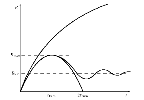
Figure 2: The evolution with time of a top–hat perturbation. The upper curve is the expansion of the exterior mass shell, while the closed curve is the solution which behaves like a closed FRW model. The wavy curve is the radius of a realistic perturbation which bounces back and virializes after few oscillations (from Kaiser 2002).

If we assume that the radius of the virialized halo is about half of the radius of maximum expansion, the reader should be able to derive the actual average density contrast within the virialized halo with respect to the ambient density, as well as the linear value of the density contrast at the time of collapse. This can be left as a useful exercise, in the simple case of an EdS universe (see Kaiser 2002 for the solution and much more on cosmic stucture formation). It turns out that the linear threshold for collapse in an EdS universe is $\delta_{c0}=1.686$, while the actual density contrast of a virialized halo is $\Delta_{vir}=178$. These numbers, particularly the linear threshold, generalized for different choices of the cosmological parameters, will be relevant for the following analysis. One may wonder how few magic numbers can describe a plethora of complex physical processes. However, as we will see, these numbers allow us to make several predictions, whose reliability is supported by numerical experiments. We have many reasons to proceed confidently.

1.4 Clusters of galaxies reflect the expansion rate of the Universe

As we saw, the expansion rate of the Universe, entering equation 5, affects the evolution of the linear perturbations. It follows that the growth of a perturbation is slower when the expansion is faster. The Hubble parameter in its general form writes $H(z)=H_{0}[\Omega_{0}(1+z)^{3}+\Omega_{k}(1+z)^{2}+\Omega_{\Lambda}(1+z)^{3+3w}]^{1/2}$, where $w$ is the ratio between the pressure and the energy density in the equation of state of the dark energy component (Caldwell et al. 1998). The special case $w=p/\rho=const=-1$ corresponds to the quantuum vacuum energy, aka the cosmological constant. We find that in a low density Universe the expansion is faster than in the EdS case, so we expect that clusters form much later for the same initial conditions. We have a situation more similar to a low density Universe in the case of a flat Universe with cosmological constant. This last case is the favorite choice, since today many observational evidences tell us that the Universe is accelerating (as shown in several lectures at this School), and in the context of general relativity, this can be explained by the presence of dark energy.

Therefore, if we set the initial conditions and the cosmological parameters, we can predict the redshift when virialized halos of a given mass are expected to form. At this point we can reverse the problem: given a measure of the initial conditions (the fluctuations in the CMB are providing them at a redshift $z\sim 1500$) and after counting clusters of galaxies at each redshift, we can infer the expansion rate of the Universe and therefore the cosmological parameters. Clusters are much more useful for this kind of test than, for example, galaxies, since they are the largest virialized structure in the universe, therefore the closest to the initial linear spectrum of density perturbations and most affected by the expansion rate.

To play this game, obviously we should not focus on single objects, rather we should measure the evolution of the number density of clusters with the cosmic epoch and their distribution with mass. Let’s see this in detail.

1.5 Where cosmological parameters enter the game

We are interested in the statistical properties of the initial conditions, in other words, to the average value of $\delta$ on a given scale. Since the majority of inflationary models predict that the fluctuations in the density field $\rho$ should be Gaussian, we need to know only its variance. To define operationally the variance on a given scale, we can imagine to smooth the linear field by measuring the overdensity around each point in space within a sphere of radius $R$ (the top–hat filter function). Since the density field is linear, a spatial scale is related to a mass scale simply by $M=(4\pi/3)\rho_{0}R^{3}$ where $\rho_{0}$ is the average density. If we express the fluctuations field in terms of its Fourier power spectrum $P(k)$, the variance reads:

$$\sigma^{2}(M)={1\over{8\pi^{3}}}\int W^{2}(kR)P(k)d^{3}k\,,$$ (8)

where $W(kR)$ is the filter function in the Fourier space. The filter function corresponding to a top–hat in real space is oscillating due to the sharp edges (see Kolb & Turner 1990, Kaiser 2002). Since every mode grows independently from each other in the linear regime, we expect that $\langle\delta\rangle$ is proportional to the linear growth factor $D(t)$. If we call $\delta_{c}$ the critical value corresponding to the collapse, the epoch of collapse of an overdensity of a mass $M$ is implicitly defined by the relation:

$$\sigma(M)D(z_{coll})=\delta_{c}\,.$$ (9)

The linear growth factor $D(z)$, which we know since it is the solution of equation 5, can be written in a generic cosmology as follows (see Peebles 1993):

$$D(z)={5\over 2}\Omega_{0}E(z)\int^{\infty}_{z}{{1+z^{\prime}}\over{E(z^{\prime})^{3}}}dz^{\prime}\,,$$ (10)

where $E(z)\equiv H(z)/H_{0}$. In the general case it is not possible to invert analytically equation 9. Again, since we are still in the theoretical mood, we can assume the EdS case and enjoy its analytical formulae (as you see, simplicity sometimes attracts theoreticians against any evidence!). Another useful step is to approximate the linear spectrum of the density perturbations with a power law, $P(k)\propto k^{n}$ with $n\simeq-1;-2$. In this case, from equation 8, $\sigma(M)\propto M^{-a}$ with $a=(n+3)/6>0$. Since the linear gowth is $D(t)=(t/t_{0})^{2/3}=1/(1+z)$, we easily can invert the condition $D(t)\sigma(M)=\delta_{c}$ to obtain the typical mass which is collapsing at a given epoch:

$$M_{c}(t)=M_{c0}(t/t_{0})^{4\over{n+3}}\,.$$ (11)

Here we meet a fundamental property of any model based on CDM: the hierarchical clustering. For any $\sigma(M)$ which is decreasing with mass (which implies $a>0$, or $n>-3$), more massive objects form at later times. The hierarchical clustering, i.e., the progressive assembling of larger and larger structures with cosmic time, is the direct consequence of this property. Actually, the preferred choice is the spectrum for adiabatic fluctuations in a CDM universe, and it is the result of a detailed computation involving fluid equations for relativistic and non–relativistic components in an expanding universe (see the software CMBFAST, http://cmbfast.org/, by U. Seljak and M. Zaldarriaga). Unsurprisingly, a realistic CDM spectrum is not as simple as a power law. The resulting $\sigma(M)$ shows a varying slope as shown in Figure 3.

see fig3.gif

Figure 3: The typical value of the linear fluctuations $\sigma(R)$ predicted for an $\Omega_{0}=0.3$, $\Omega_{\Lambda}=0.7$ Universe compared with the values obtained from observations on different scales (from Tegmark 2002). See lectures by W. Percival for constraints from SDSS, and by R. Caldwell for constraints from the CMB).

Before ending this section, we remark that few years ago, the hierarchical clustering hypothesis was not so radicated into cosmological models. Imagine that we have a kind of dark matter which has no power at all at small scales. From equation 8, it is easy to see that $\sigma(M)=const$ below some threshold $M<M_{th}$. As a consequence, all the scales with $M<M_{th}$ collapse at the same time. If $M_{th}$ is large enough, let’s say the scale of a cluster of galaxies, then clusters form at the same time or even before galaxies. This is the situation we have when we consider light particles like massive neutrinos as candidates for dark matter. Now we know that neutrinos give a negligible contribution to the density of the Universe (see Lahav & Liddle 2006). Given the success of the CDM spectrum in reproducing observations on several scales (as shown in Figure 3) the common wisdom is that cosmic structures follow hierarchical clustering, at least as far as dark matter is concerned (but beware of the baryons!).

1.6 The mass function

Now we can predict the typical mass scale which is virializing at a given redshift. Is this enough to efficiently constrain the cosmological parameters? Not yet: we can work out much better observables which will allow us to perform efficient cosmological tests. The important step we have to take now is to derive the mass function. To do that, first we must write the probability distribution of the fluctuations $\delta$, which we already assumed to be a Gaussian with dispersion $\sigma$:

$$P(\delta)={1\over{\sqrt{2\pi}\sigma}}exp\{{1\over 2}\delta^{2}/\sigma^{2}\}\,.$$ (12)

Since we are dealing with a linear field, it seems safe to say that the fraction of mass which is in regions with overdensity larger than a given $\delta$, is equal to the fraction of volume that, filtered with our top–hat filter of size $R$, is overdense above the same threshold. This fraction is simply the integral of the Gaussian from the overdensity threshold up to infinity. If we set $\delta_{c}(z)=\delta_{c0}\times D(0)/D(z)$, we obtain the fraction of mass which is in virialized halos at a given epoch $z$. This condition reads:

$$N(M)MdM=\int_{\delta_{c}(z)}^{\infty}P(\delta,\sigma(M))d\delta\,,$$ (13)

where $N(M)$ is the number density of virialized halos in the mass range $M$ and $M+dM$. Then we can obtain an expression for $N(M)$ simply deriving the integral on the right hand side with respect to mass:

$$N(M)={{\rho}\over{M}}{d\over{dM}}\int_{\delta_{c}(z)}^{\infty}P(\delta,\sigma(M))\,.$$ (14)

Our tidy theoretical attitude is rewarded again: the solution is analytic. Leaving the mathematics to the reader, we write the final, famous result, the Press & Schechter (PS) mass function (1974):

$$N(M)\,dM\,=\,\sqrt{{2\over\pi}}{\rho\over M}{{\delta_{c}(z)}\over{\sigma^{2}}}{{d\sigma}\over{dM}}\,exp\Big{(}-{{\delta_{c}(z)^{2}}\over{2\sigma^{2}}}\Big{)}\,dM\,.$$ (15)

Its typical shape is characterized by a power law at low masses, and an exponential cutoff at large masses. Given its simplicity, its success is often referred as the Press & Schechter miracle.

1.7 Is the Press & Schechter approach accurate enough?

Unfortunately miracles are not allowed in science. You may think that this approach is just a didactical exercise to understand the basic concepts, while cosmologists actually use terribly complicated formulae or awfully long numerical computations for the mass function. Well, the truth is that this formula is still at the core of the majority of the works deriving cosmological parameters from clusters of galaxies. Indeed, many numerical experiments (N–body simulations) actually support the validity of the PS approach. Clearly, some differences with respect to the original PS approach were found. Discrepancies are mostly due to the many non linear effects which are not included in the PS formalism. A recent example of a comparison between N–body and the PS formula is shown in Figure 4. We note that the PS formula tends to underestimate the number density of halos at very high redshift. However, if we consider that clusters are observed today up to redshifts slightly above 1, we have to admire the remarkable similarity with the results from the time–expensive, brute–force approach of N–body simulations.

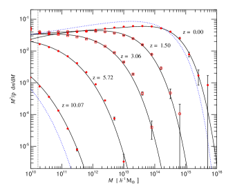
Figure 4: The Press & Schechter mass function (dotted lines) tested against N–body simulations (dots and solid lines, from Springel et al. 2005).

To improve the PS model, some empirical fitting formulae were proposed on the basis on N–body simulations (Jenkins et al. 2001). However, this approach is heavy, because in principle it requires a new simulation every time the cosmological parameters are varied. The PS mass function has the great advantage that the cosmological parameters space can be explored rapidly. Finally, I just mention here that the PS formalism can be extended to give complete merger histories of single halos (Lacey & Cole 1993), conditional probability function of progenitor halos (Bower 1991), biased distribution of halos within halos (Mo & White 1996), all topics we do not explore here, but that proved to be very useful in interpreting data. As a final comment, the PS approach after more of 30 years, is still extensively used in the large majority of the papers on precision cosmology with clusters of galaxies.

1.8 From the mass function to the distribution of observables

Let’s take a closer look to the behaviour of the mass function. We identify two sets of ingredients: the initial conditions (normalization and shape of the power spectrum) entering $\sigma(M)$, and the cosmological parameters ($\Omega_{0}$, $\Omega_{\Lambda}$, $w$) entering $\delta_{c}(z)$ and the overall normalization of the mass function. As you can easily see, the exponential cut off at the massive end is where the function is most sensible at both sets of parameters, through the normalization of the power spectrum (expressed conventionally as $\sigma_{8}$, which is the amplitude of the spectrum at the scale of $8h^{-1}$ Mpc), and the linear growth factor. We can now see in much more detailed terms the behaviour we already appreciated qualitatively: the evolution of cosmic structures is slower in a universe with lower density with respect to and EdS universe; the same for a $\Lambda$–dominated, flat universe. In quintessence models, for higher values of the parameter $w$, the growth ceases earlier. If we normalize our mass function in order to have the same local density of clusters today, the evolution with $z$ appears faster for $\Omega_{0}=1$ than for open or $\Lambda$–dominated universes. This is shown visually by the N–body simulation in Figure 5 (upper panel). Quantitatively, the expected evolution of the number density of massive clusters (with virial mass $M>5\times 10^{14}h^{-1}M_{\odot}$) is also shown in Figure 5 (lower panel). Now our observational side can take over, and note that, after all, an EdS universe is not more appealing than a low density one since, after all, in the last case we expect much more clusters at high redshifts. And observers love to find high–redshift objects.

see fig5.gif

Figure 5: Top: clusters of galaxies (circles) in an N–body simulation for an EdS universe (bottom panels) compared with clusters in an open FRW universe, with statistically equivalent conditions at $z=0$. The evolution backward in time of the mass function is strikingly different (Borgani & Guzzo 2001). Bottom: the evolution of the number density of clusters with virial mass $M>5\times 10^{14}h^{-1}M_{\odot}$ for different choices of the cosmological parameters (Rosati, Borgani & Norman 2002).

We are almost ready to handle real data, except for a final, small step, which consists in a simple change of variables. As you know, in most cases we do not measure directly the virial mass. What an astronomer typically measures is the emitted light in a given band. In our case, as we will see shortly, we will focus on measuring the total luminosity $L$ in the X–ray band and the virial temperature $T$ of the diffuse gas. Therefore, we prefer to have a prediction for the luminosity or the temperature function. This is straightforward if we have a relation $M$–$L$ or $M$–$T$. We know, from the virial theorem, that these relations can be obtained from our spherical collapse model. Once we have the relationships between the observables and the mass, we can write the luminosity (XLF) and the temperature (XTF) functions as:

$$\Phi(L)dL=N(M){{dM}\over{dL}}dL\,,\,\,\,\,\,\,\Phi(T)dT=N(M){{dM}\over{dT}}dT\,.$$ (16)

Enough theory.

2 From Observations to Cosmological Parameters

2.1 The observer’s mood

We can start the second part of this lecture, where we will encounter different kind of problems. We are about to look at data, therefore we will face reality, which is always somewhat shocking when coming from the ideal, linear and spherical world of theory.

As we already know, we need a good measure of the actual number density of clusters of galaxies as a function of mass and redshift. We also know that we will get the luminosity or, in the best case, the temperature function of clusters. This implies that we need to be able to: find clusters, measure with high accuracy the quantity of interest, and define the completeness of our survey. Completeness is a key quantity in observational cosmology. A well defined completeness means that, for the solid angle of the sky covered by our survey, we are able to detect all the objects with luminosity (or temperature, or mass) above a given value and within a given redshift. This is mandatory to compute the volume we actually explore in the survey and, therefore, the comoving number density. Needless to say, a survey with few objects but a well defined completeness is way much better than a survey with hundreds of objects but a poorly defined completeness. Therefore, we need a strategy to find as many clusters as possible with a well defined completeness. Which is the best observational window to do that? Let’s start examining some options.

2.2 Optical band

Searching for clusters in optical images is basically counting galaxies and looking for overdensities with respect to the background value (see Gal 2006 for a review). In doing this, the optical colors of the member galaxies are a very useful information. Passive, red galaxies preferentially populate the central regions of clusters, and they form a well defined color–magnitude relation. A galaxy selection picking the reddest galaxies in the field, helps in reducing the contamination by the field galaxies. These techniques can give efficient clusters detection out to $z\geq 1$ (see Gladders & Yee 2005).

Optical surveys are very convenient to find many cluster candidates. We remind that clusters are rare objects (especially the massive ones) and therefore we need to survey large area to find many of them. The optical band offers the opportunity to cover wide area with large CCD frames, coupled to the availability of ground–based telescopes with large field of view. However optical observations have the drawback of a difficult calibration of the selection function, and therefore the completeness of an optical survey of clusters is very hard to define. This is because the detectability of a cluster depends on the luminosity, the number, and the concentration of its galaxies, three aspects that can vary from cluster to cluster. In addition, projection effects cause severe contamination from background and foreground galaxies: filamentary structures and small groups along the line of sight can mimic a rich cluster. For the same reason, in the presence of a positive fluctuations of the background galaxies, moderately rich cluster can be missed.

More troubles when we try to relate the optical light to the total mass. The total optical luminosity of a cluster is somehow proportional to the total mass. But we know that the stellar mass in the galaxies represents a tiny fraction of the total, and usually only the brightest galaxies are detected, so that a lot of stars in small, undetected galaxies must be accounted for, by assuming a model for the galaxy luminosity function. So, we should not be surprised to know that the relation between the total optical luminosity of a cluster and its total mass is very loose. In order to obtain an accurate measure of the mass, we may use optical spectroscopy to measure the velocity dispersion of the galaxies and then apply the virial theorem. However, this requires a lot of observing time, and obviously it is still affected by contamination from interlopers. All these problems become more severe at high redshift, as the field galaxy population overwhelms galaxy overdensities associated with clusters. A completely different technique is to measure the mass directly through strong and weak lensing (see, e.g., Dahle et al. 2003). This is a very promising tool, but it has its own problems, like severe projections effects (the lensing depends on all the mass along the line of sight towards the clusters and on its position) and the difficulty to obtain clean lensing signal.

2.3 Millimetric band (SZ effect)

Among the many virtues of clusters of galaxies, there is this peculiar feature: clusters can be seen as shadows on the cosmic background radiation. This is due to the Sunyaev–Zeldovich (SZ) effect (Sunyaev & Zeldovich 1972). We know that most of the baryons in clusters are in the form of very hot, ionized gas. Photons from the CMB passing through a cluster find many high–speed electrons and therefore experience Inverse–Compton scattering. In this process, the energy is transferred from the electrons to the much colder CMB photons. Since this process preserves the number of photons, the net result is that the black–body spectrum of the CMB is slightly distorted and shifted to larger frequencies by an amount that depends on the temperature, and on the column density of the ICM. The net effect on the CMB is the production of a cold spot at low and a hot spot at high frequencies, where the pivotal frequency is about 217 GHz (see Holder & Carlstrom 2001). This sounds very promising, since we have both a spatial and a spectral signature. Actually, several clusters have been imaged with the OVRO and BIMA arrays (Carlstrom et al. 2002). Indeed, the scientific community is making a strong effort to build instruments that can study both CMB and the SZ effect from the ground (like AMI, ACT, AMiBA, APEX, SPT), or from space (like the Planck satellite, whose full–sky survey is expected to detect thousands of clusters).

Among the positive aspects of SZ observations, we find the absence of the redshift dimming, which allows one to identify clusters virtually at any redshift. This means that the selection criteria are essentially equivalent to a completeness in mass, which is very desirable. However, severe contamination from foreground and background radio sources is expected. Multi–frequency observations can help a lot in disentangling the spectral signature of the SZ effect from the spectrum of radio sources. However, the difficulties in detecting clusters via the SZ effect are still significant (see Birkinshaw & Lancaster 2004). An easy prediction is that in five years, the SZ effect will be one of the main observational window to find and study clusters of galaxies.

2.4 X–ray band

At present, in my view, the X–ray band is the most convenient to find and investigate clusters. Anyway, it is the field in which I spent most of my activity, and therefore, for a mix of objective and private reasons, since now on, I will focus mostly on X–ray.

The first thing to say is that clusters appear as strong–contrast sources in the X–ray sky up to high redshifts, thanks to the dependence of the X–ray emission on the square of the gas density (see §2.5). Given the relatively small number of sources, X–ray images of clusters are virtually free from contamination from foreground and background structures. In other words, clusters are the second most prominent sources in the X–ray sky (after Active Galactic Nuclei), at striking difference with the optical and millimetric bands where they have to struggle to emerge above other stronger signals. This can be clearly appreciated in Figure 6 (left) where almost all the point sources in the image are AGN, while the bright, extended source in the center is a cluster at $z=0.79$. The image has been taken with the ACIS–I detector, covering a square of 16 arcmin by side. X–ray emission from clusters can be detected up to redshift larger than one, as shown in Figure 6 (right) where the X–ray emission (red) from the $z=1.235$ cluster RXJ1252 is shown on top of the optical image.

see fig6.gif

Figure 6: Left: The cluster MS1137, $z=0.79$, in a field observed for 116 ks with the X–ray telescope Chandra. The cluster is the bright extended source in the center, while most of the remaining sources are AGN. Right: the X–ray emission from the $z=1.235$ cluster RXJ1252 is shown on top of the optical image taken with the VLT telescope (Rosati et al. 2004).

A flux–limited X–ray survey can provide a sample of clusters with a well defined completeness, thanks to the fact that the X–ray emission from clusters is continuous (at variance with the optical emission associated to the single galaxies) and centrally peaked towards the center. Therefore we just need to establish a robust connection between the X–ray luminosity and the total mass. A potential problem with X–ray clusters is that the X–ray flux is sensitive to irregularities in the gas distribution. However, this problem does not seem dramatic, given that most of the clusters appear smooth and round, and the theory provides us with a robust connection between the total mass and the ICM properties. Thus, for the moment, we just need to fully appreciate the advantages in looking at clusters with X–ray satellites, which became possible since the 60s thanks to the first X–ray missions leaded by Riccardo Giacconi. In the spirit of constraining the cosmological parameters, X–ray surveys of clusters of galaxies had a large success in the 90s, thanks to ROSAT and other satellites, and provided consistent but sometimes debatable results. For a review of the many surveys with cosmological impact see the review by Rosati, Borgani & Norman (2002).

We are now in the era of the XMM–Newton and Chandra satellites. These two telescopes are mostly performing pointed observations of clusters discovered in the previous surveys. No wide area surveys are currently planned, given the small field of view of these satellites (nonetheless, some serendipitous surveys are underway with both of them). These pointed observations are bringing to us many beautiful images, along with many unconfortable news that we will discuss in §3. Before stepping further, let’s remind the basics of X–ray emission from the ICM.

2.5 The X–ray emission from Clusters of Galaxies

We know that most of the baryons in clusters are in the form of hot plasma. This plasma is optically thin and it radiates by free–free (bremsstrahlung) emission. It is in collisional equilibrium, therefore its typical temperature is set by the large dynamical masses of clusters ($10^{14}-10^{15}M_{\odot}$) to be in the range of 10–100 millions K (corresponding to 1–10 keV). This implies that most of the emission is in the X–ray band. The total X–ray emissivity due to thermal bremsstrahlung is obtained by integrating over the distribution of speeds of the plasma electrons, and, after a further integration over frequencies, it can be written as (see Ribicky & Lightman 1979):

$${{{dL}\over{dV}}~{}=~{}1.4\times 10^{-27}\,T^{1/2}\,n_{e}^{2}\,Z^{2}\,\bar{g}_{B}~{}{\tt erg\,s^{-1}cm^{-3}}}\,,$$ (17)

where $Z$ is the atomic number of the ions and $\bar{g}_{B}$ is the velocity–averaged Gaunt factor averaged over frequencies. First, we notice the dependence of the total emissivity on the square of the electron density. This is the main reason why clusters are high–contrast sources in the X–ray sky, and also why superposition or confusion effects due to smaller background or foreground halos, are less important than in the optical band, where the total luminosity scales linearly with the (stellar) mass. We also note the weaker dependence on the temperature ($T^{1/2}$).

Another contribution to the X–ray luminosity comes from the line emission due to heavy ions. This contribution is generally negligible in terms of total emission, since at temperatures larger than 5 keV, almost all the heavy nuclei are fully ionized. However, the line–emission contribution is increasing at low temperatures, and starts to be relevant below 2 keV. This aspect is important when studying the production of metals in cluster galaxies and their diffusion into the ICM. A typical X–ray spectrum of a cluster, with the typical Iron line at 6.7 keV rest–frame, is shown in Figure 7 (right).

Figure 7: The spectrum of MS2137 observed with ACIS-I onboard of the Chandra satellite. MS2137 is a bright X–ray cluster at z=0.313, with an average temperature of about 5 keV.

Equation 17 gives the luminosity per unit volume, therefore, the total luminosity must be obtained by integrating up to the virial radius. In the simplest assumption of isothermality ($kT=const$ at any radius in the cluster), the only relevant quantity is the square of the electron density $n_{e}^{2}(r)$, which is generally assumed proportional to the gas density $n_{g}$. In general the gas density profile is described with the so–called $\beta$–model (Cavaliere & Fusco Femiano 1976), which consists in a flat central core and a steep decrease in the outer regions:

$$n_{g}\propto 1/(1+(r/r_{c})^{2})^{3\beta/2}\,,$$ (18)

where $r_{c}$ is the core radius, and the parameter $\beta\sim 0.5$–$1$ can be interpreted as the ratio of the specific energy of the dark matter particles (often measured through the galaxies velocity dispersion) over the gas temperature. Given the steep slope outside the core, and the $n_{g}^{2}$ dependence of the luminosity, only the central regions (few core radii) are clearly detected in the X–ray images. The outer regions are hardly detected even with present–day satellites. Observers often prefer to quote all the quantities within the observed radius, which is typically half or less than the virial one.

As we know, X–ray detectors onboard of the Chandra and XMM satellites are CCD cameras, which read the collected photons every few seconds, recording both the position and the energy (with a reasonable error of few percent). Therefore X–ray astronomy has the big advantage of recording images and spectra at the same time. High resolution X–ray spectroscopy is still feasible through gratings, however the energy resolution of the CCD is good enough to our purposes of measuring the temperature of the baryons.

Once we obtain the baryon density from the X–ray surface brightness, and the temperature of the gas, we can measure the total mass simply by applying the condition of hydrostatic equilibrium:

$$M(<r)=-{{k_{B}TR}\over{G\mu m_{p}}}\Big{(}{{d{\tt log}(\rho_{g})}\over{d{\tt log}(r)}}+{{d{\tt log}(T)}\over{d{\tt log}(r)}}\Big{)}\,,$$ (19)

where $\mu$ is the mean molecular weight ($\mu\sim 0.6$) and $m_{P}$ is the proton mass (see Rosati, Borgani & Norman 2002). Here we let the temperature free to change with the radius. Of course this equation is particularly simple in the isothermal case. In general, the masses obtained in this way are pretty close to that obtained simply through the virial theorem $T\propto M^{2/3}$. On the other hand, it is well known that clusters do have a temperature structure, which is often well described by a mild decrease outwards (see Vikhlinin et al. 2005), and, in more than half of the local lcusters, a drop of about a factor of three in the very inner regions (the cold core, see Peterson & Fabian 2005). The temperature profile is quite important, but its measure is increasingly difficult at increasingly high redshifts. Indeed, we need a lot of photons in order to measure the temperature in several concentric regions (at least one thousand for each independent spectrum), and to obtain the deprojected temperature profiles. For this reason, virial masses of distant clusters are often derived assuming isothermality.

Our framework allows us to relate the basic X–ray observables, luminosity and temperature, to the dynamical mass. We already know that luminosity is more affected by the details of the gas distribution, while the $M$–$T$ relation appears more stable since it is directly based on the virial theorem. But we also know that luminosity is much easier to measure, since we need much less photons to measure a luminosity, and therefore we can observe many more clusters within a given amount of telescope time. A shortcut is to build phenomenologically the $L$–$T$ relation, fitting the data with a formula of the kind:

$$L_{bol}=L_{6}\Big{(}{{T_{X}}\over{6keV}}\Big{)}^{\alpha}(1+z)^{A}\Big{(}{{d_{L}(z)}\over{d_{L,EdS}(z)}}\Big{)}^{2}10^{44}h^{-2}ergs^{-1}\,,$$ (20)

where $\alpha$ is measured to be about 3, while the evolutionary parameter $A$ is more uncertain and varies between 1 and 0 (see Vikhlinin, et al. 2002, Ettori et al. 2004). Once the relations between the X-ray observables and the mass are established, we can compare the observed XLF and XTF to our predictions. For a review of the X–ray properties of X–ray clusters, see the book by Sarazin (1988).

2.6 Measuring $\Omega_{0}$ from the observed X–ray luminosity function

The luminosity function seems easy to measure: first we count all the clusters in our survey, then we measure their flux just counting the photons from each cluster. We also have to know the redshift of each cluster with a good approximation, in order to compute luminosities. The redshift can be obtained with an optical spectroscopic follow–up on a limited number of member galaxies, or with photometric techniques. As noted before, shallow X–ray surveys allows us to measure the luminosity with good accuracy, and to scan a wide area of the sky. Once we have a flux limited sample with measured luminosities, we build the XLF by adding the contribution to the space density of each cluster in a given luminosity bin $\Delta L$ :

$$\phi(L_{X})={1\over L_{X}}\Sigma^{n}_{i=1}{1\over{V_{max}(L_{i},f_{lim})}}$$ (21)

where $V_{max}$ is the total search volume defined as:

$$V_{max}=\int_{0}^{z_{max}}S[f(L,z)]\Big{(}{{d_{L}(z)}\over{(1+z)}}\Big{)}^{2}{{c\,dz}\over{H(z)}}\,,$$ (22)

where $S(f)$ is the sky coverage, which depends on the flux (since the sensitivity of a survey can vary across the surveyed region of the sky), and $d_{L}(z)$ is the luminosity distance.

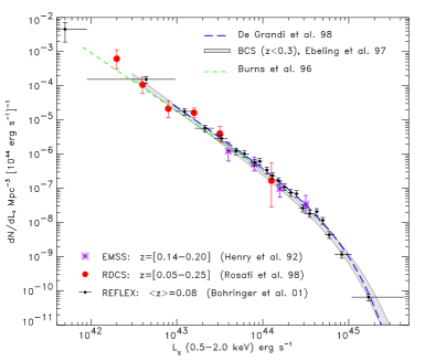
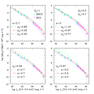
Figure 8: Upper panel: the local X–ray luminosity function of clusters of galaxies from different samples computed for an EdS Universe with $H_{0}=50$ km s^-1 Mpc^-1 (Rosati, Borgani & Norman 2002). Lower panels: the local X–ray luminosity function of clusters of galaxies from RDCS (filled circles) and BCS (open circles) for different $\sigma_{8}$ and different parameter $\alpha$ for the slope of the $L$–$T$ relation (Borgani et al. 1999)

Remember that we expect to get information on the cosmological parameters both from the shape of the XLF and from its evolution with redshift. To begin with, the shape of the local XLF is well understood thanks to several different surveys giving consistent values, and it is shown in figure 8 (upper panel). This allows already to get some information from the data at $z=0$, by finding the parameters which minimize the $\chi^{2}$ computed on the binned luminosity function from equation 21, or by a maximum–likelyhood approach using the unbinned data (see Borgani et al. 2001).

However, when only local data are used, we find a lot of degenaracy among cosmological parameters. Lower $\Omega_{0}$ can be compensated by higher spectrum normalization $\sigma_{8}$ (see Figure 8, lower panels). To break this degeneracy we can use the evolution with redshift. The evolution of the XLF is still debated: there is a hint of evolution at the very bright end, but for the typical $L_{*}$ clusters and less luminous ones, there is no evolution almost up to $z\sim 1$ (see discussion in the review by Rosati, Borgani & Norman 2002). In other words, most of the clusters, if we exclude the brightest ones, are already in place at high redshift. We know what does it mean, at least qualitatively: the matter density parameter $\Omega_{0}$ is significantly lower than 1.

Our group, few years ago, applied this cosmological test to the RDCS survey (Rosati et al. 1998), which is the deepest sample of X–ray selected clusters. This choice provide a good leverage in terms of cosmic epoch, but necessarily, given the relatively small solid angle surveyed with respect to shallower surveys, does not probe well the high luminosity end. The results, published by Borgani et al. (1999; 2001) are shown in Figure 9, where we used also data from the EMSS survey (Gioia et al. 1990). In these Figures we notice that some degeneracy is still present also when fitting the XLF in the high redshift bins. We also notice that the constraints on the cosmological parameters $\Omega_{0}$ and $\sigma_{8}$, are weakened when the parameters $\alpha$ and $A$, describing the slope and evolution of the $L$–$T$ relation, are allowed to vary within the observational uncertainties.

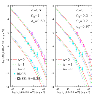
Figure 9: The X–ray luminosity function of clusters of galaxies in three different redshift bins: z=0.3–0.6 (EMSS data); z=0.25–0.50 and z=0.50–0.85 (RDCS). For each model and at each redshift, different curves refer to different evolutions for the $L$–$T$ relation (Borgani et al. 1999).

The uncertainties on the cosmological parameters are better shown in terms of confidence contour levels, where we can also evalutate the effects of the uncertainties associated to the parameters describing the $L$–$T$ relation. 5In Figure 10 we show how the confidence contours in the $\Omega_{0}$–$\sigma_{8}$ space dance around when the slope and evolution of the $L$–$T$ relation (parametrized by $\alpha$ and $A$ like in equation 20), but also the normalization of the $M-T$ relation (parameter $\beta$), are allowed to vary. The displacements of the contours are at more than 3 $\sigma$, therefore we are learning unconfortable news: the uncertainties on the properties of the ICM are affecting the cosmological tests at a significant level.

The situation is getting worse when we investigate the dark energy parameter $w$. While the density parameter $\Omega_{0}$ is well constrained by clusters, $w$ is hardly constrained at all. Recent works trying to constrain dark energy, combine constraints from both SneIa and clusters, to significantly improve the constraints on $w$ due to the complementarity of the two tests in the $\Omega_{0}$–$w$ space (see Figure 11).

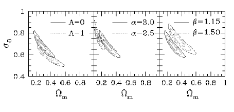
Figure 10: Confidence contours in the density parameter $\Omega_{0}$ and the normalization of the density fluctuations spectrum $\sigma_{8}$ from the fit of the high–z XLF for different choices of the parameters describing the physical relations $L$–$T$ ($\alpha$ and $A$) and $M$–$T$ ($\beta$; Borgani et al. 2001).

Figure 11: Confidence contours (1–3 $\sigma$ levels for two degrees of freedom) in the $\Omega_{0}$–$w$ plane obtained from SNeIa only (Perlmutter et al. 1999 sample, left panel) and SNeIa plus REFLEX (right panel, from Schuecker et al. 2003).

2.7 Measuring $\Omega_{0}$ from the observed X–ray temperature function

At this point you may ask: since our theoretical framework seems quite successful, why do we have such large uncertainties in the relations between $L$ and $T$? Not only we showed that the relation between mass and luminosity is reasonably understood on the basis of the spherical collapse, but we also mentioned a possible shortcut through the direct measure of the $L$–$T$ relation. Well, we knew that something wrong were lurking somewhere… However, before worrying too much, let’s give a try to the XTF, which is based only on the more robust $M$–$T$ relation. Indeed, the $M$–$T$ relation relies directly on the virial theorem and it is observed to have smaller scatter with respect to that observed in the $L$–$T$ relation.

When using the XTF, the price to pay, as we know, is that it is much more difficult to assemble a complete sample of clusters with temperatures measured with reasonable errors. However the XTF is considered to be more effective in constraining cosmological parameters. The first good news is that the constraints from the XTF are similar to that from the XLF. The constraints obtained from the XTF point towards $\Omega_{0}\sim 0.3$ for a flat universe (see Donahue & Voit 1999), providing at the same time significant constraints on the normalization of the power spectrum (see Pierpaoli et al. 2001). In Figure 12 we show the results from Eke et al. (1998). We notice the tight constraints, but, again, also a significant degeneration in the $\sigma_{8}$ –$\Omega_{0}$ space.

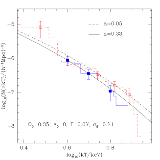
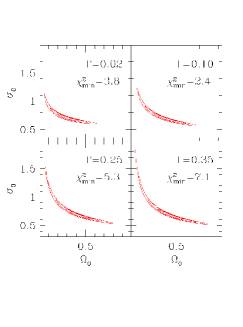
Figure 12: Left: Fit to the evolved temperature function. Right: confidence contours in the $\Omega_{0}$–$\sigma_{8}$ space (from Eke et al. 1998).

An additional problem comes from a parameter which we considered, so far, pretty robust: the normalization of the $M$–$T$ relation. It has been noticed that the value of $\beta$ found in N–body simulations is higher than the observed one. This can be due to several effects (see Borgani et al. 2004), but the net result is that the uncertainties on this parameter introduce uncertainties in the constraints from the XTF in the same way as the $L$–$T$ parameters are weakening the constraints from the XLF (see, e.g., Ikebe et al. 2002).

It is clear at this point that the main uncertainties comes from the poor understanding of the scaling relations between the ICM observables and the mass, both from the theoretical and the observational points of view. A detailed investigation of the effects of such uncertainties is given in Pierpaoli et al. (2003). They conclude that the cosmological constraints from XLF and XTF, both the local and the evolved ones, are reliable and consistent with each other, but that the statistical errors on the cosmological parameters are larger than previously thought. The buzzword now is: we need to improve the quality of the data on single clusters to better understand the physics of the ICM. But why did clusters prove to be such a difficult topic, after being the best candidate for the most friendly objects in the Universe?

3 New Physics and future prospects

3.1 Something is missing: new physics for the clusters baryons

Why do we have such a poor understanding of the $L$–$T$ relation? From equation 17, assuming $n_{e}\propto\rho_{tot}$ (in other words, that the baryons follow the total matter distribution), and integrating over the volume, we obtain $L\propto T^{2}$ (without including line–emission). This is the $L$–$T$ relation predicted in what is called the self–similar scaling (Kaiser 1986). As long as the baryons are distributed in the same way of the total mass, each X–ray observable scales like some power of the mass. Another way to say this, is that small clusters are the mass–rescaled version of massive clusters.

So far, we reasonably expected that the thermodynamics of the ICM, being dominated by dark matter, is driven by gravitational processes, like shocks and adiabatic compression occuring during the virialization phase and the subsequent growth in mass by accretion. This self–similar behaviour is also supported by N–body hydrodynamical simulations which do not include radiative cooling. But the observed slope of the $L$–$T$ relation is much steeper then predicted ($\alpha\geq 3$ rather than 2 or lower when line emission is included) and it constitutes the first strong evidence of something wrong in the self–similar picture. That’s why when performing the cosmological tests, we avoided this inconsistency by varying the parameters of the ICM scaling relations.

However, we learned that thawing the thermodynamic parameters introduces large uncertainties in the cosmological constraints. Obviously, we would appreciate a lot to have a physical basis for the observed scaling relations, in order to better control the uncertainties due to a poor description of the ICM thermodynamics. The first step is to invoke a physical process that leads naturally to an $L\propto T^{3}$ scaling, in other words, a process which implies a progressive decrease of the X–ray luminosity at low mass or temperatures, as shown in Figure 13 (top). How can we obtain this? We know that we can efficiently decrease the predicted luminosity by imposing a lower density in the central regions of the clusters. To do that, we simply need to add an extra pressure, or some extra amount of energy in the center of clusters. Extra means in excess with respect to the energy acquired through shocks and adiabatic heating. This extra energy does not translate in an higher temperature; what happens, is that the pressure increases, and the gas distribution gets puffier, readjusting itself in the dark matter potential well. A useful quantity to describe such behaviour is $K\equiv T/n^{2/3}$. This is the normalization of the equation of state of the ICM, which is that of a perfect gas, $p=K\rho^{5/3}$. We remind that the entropy is $S=Nln(K)$. The entropy is also a very convenient thermodynamic variable, since it is constant during adiabatic compression, and it changes only in the presence of radiative cooling or shock heating. For this reason, another way of describing the break of the self–similarity in clusters, as shown by Ponman et al. (1999), is to plot the entropy as a function of the cluster temperature, as shown in Figure 13 (bottom).

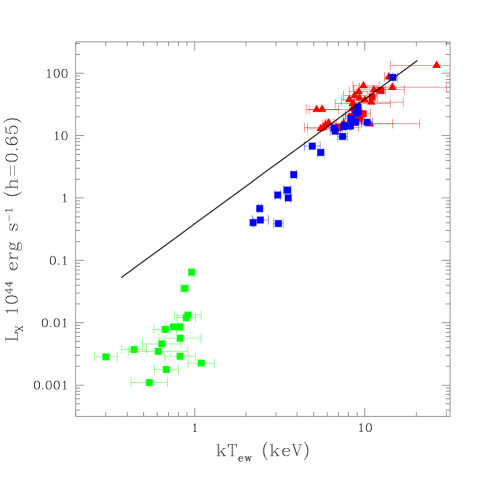
Figure 13: Top: the $L$–$T$ relation for groups and clusters showing the steeper slope with respect to the self–similar model $L\propto T^{2}$ (continuous line). Bottom: the entropy ramp, showing the higher entropy in low temperature systems with respect to the self–similar model (Voit, Kay & Bryan 2005).

The desired effect is obtained by giving about half or 1 keV to each gas particle. The effect is small in rich clusters, where the virial temperature is around 10 keV, and the energy budget is largely dominated by gravity, while it is increasingly large at lower temperatures, when the extra energy starts to be a significant fraction of the gravitational energy scale. In this way we solved the problem from the point of view of the thermodynamics (see, e.g., Tozzi & Norman 2001). Of course, the real problem starts now: which is the physical mechanism responsible for the energy (or the entropy) excess?

We have two obvious candidates which can inject energy associated to non–gravitational processes: the prime candidate is feedback from star formation processes, whose effects are testified by the presence of heavy elements in the ICM. The second candidate is feedback from nuclear activity in the clusters galaxies. Actually, the interaction of AGN jets and the ICM has been directly observed. The most spectacular example is the Perseus cluster, where jets from the central AGN (visible in the radio emission) is pushing the ICM creating two large simmetric cavities towards the center (Fabian et al. 2002; 2003; see Figure 14). Chandra and XMM added other surprises: the presence of cold fronts (Vikhlinin et al. 2001, Mazzotta et al. 2001) and of massive mergers strongly affecting the dynamical equilibrium. To this, we must add the puzzling discovery by XMM that the ICM in the central regions never cools down by more than a factor of 3 with respect to the virial temperature, despite the cooling time is much shorter than the age of the cluster. Again, another evidence that some homogeneous process heats the gas.

see fig14.gif

Figure 14: From left to right: AGN activity creating cavities in the ICM of the Perseus cluster (Fabian et al. 2002; 2003); cold fronts in Abell 2142 (Markevitch et al. 2000); an ongoing massive merger in 1E 0657–56, the bullet cluster (Markevitch et al. 2004).

Today, we see clearly that the Chandra and XMM satellites changed our perspective of clusters of galaxies. If in the ROSAT era the main goal was to find as many clusters as possible with the aim of constraining cosmology, in the Chandra/XMM era the goal is to observe with much better spatial and spectral resolution the clusters previously discovered. The physics of the ICM is much more complex than expected and this forces us to reconsider all the relations between the X–ray observables and the dynamical mass. This aspect may cast some doubts on the use of X-ray clusters of galaxies as cosmological tools. One can also think to reverse the argument: the physics of the ICM is much more interesting, so let’s investigate the evolutionary properties of clusters to understand the effects of feedback processes onto the ICM, and don’t worry about cosmology.

In my view, the investigation of cosmology and of the ICM physics must proceed together. Actually, this is what is happening: if you go through the literature in the last six years, you discover indeed that there is still a strong interest in cosmological tests with clusters, which is supported by a growing amount of works on the ICM. It must be noticed in addition, that understanding the problem of the non–gravitational heating of the ICM by energetic feedback from star formation or nuclear activity, is a key issue in cosmic structure formation. Actually, feedback is the holy grail of structure formation today! If you go to a conference on galaxies, clusters, or anything on cosmic structure formation, you will hear everywhere the word “feedback”. So, rather than saying that clusters became less interesting in a cosmological perspective, I prefer to say that clusters became even more important to understand both structure formation and cosmology.

3.2 A simpler cosmological test

There is not enough space here to describe the most recent progress in the understanding of the ICM thermodynamics. However, I want to mention another cosmological test that appears to be simpler than that discussed so far. Instead of relying on the knowledge of the dynamics of clusters, we can focus on a much simple quantity: the baryonic fraction $f_{B}$. We simply need to measure the total mass, and count all the baryons in the form of stars and ICM. From semianalytical models and numerical simulations, we expect that the physics of the ICM does not affect $f_{B}$ if measured at a radius where the gravity dominates; therefore, it should be close to the cosmic value $\Omega_{B}/\Omega_{0}$. In other words, the baryons are allowed to behave wildly and decouple from the dark matter distribution in high density regions, but on large scales they are not displaced differently from dark matter. The virial radius is expected, then, to include a closed region where the average composition does not change during the evolution of the cluster. It is straightforward to see that the measure of $f_{B}$ and the knowledge of $\Omega_{B}$ from nucleosinthesis or from the CMB (Spergel et al. 2003) gives a straightforward measure of $\Omega_{0}$ (see White et al. 1993).

But this is not all: for the same reasons, the baryonic fraction should not evolve with redshift. However, the actual measure of $f_{B}$ does depend on the angular distance. The mass of baryons is recovered by measuring the flux and by knowing the physical size of the cluster. The relation between the messured flux $S_{X}$ and the mass of gas reads as:

$$S_{X}=L_{X}(1+z)^{-4}/(4\pi d^{2}_{ang})\propto M^{2}_{gas}\theta^{-3}_{c}d^{-3}_{ang}/d^{2}_{ang}\,.$$ (23)

On the other hand, the total mass depends on the angular distance as $M_{tot}\propto\theta_{c}d_{ang}$. It follows that $f_{B}=M_{gas}/M_{tot}\propto d_{ang}^{3/2}$. Thus, we have two advantages here: the value of the baryon density gives $\Omega_{0}$, while its apparent evolution is depending on the cosmological parameters through $d_{ang}$. Therefore, the cosmological test consists in requiring no evolution in the observed $f_{B}$. Any apparent evolution in the baryonic fraction is the smoking gun of wrong cosmological parameters. It is important to perform this test on a redshift range as wide as possible (see Figure 15, left).

This is not a dynamical test, but rather a geometrical test, and it is more sensitive to $\Omega_{\Lambda}$ (see Allen et al. 2004). However, we notice that the scatter in the baryonic fraction from cluster to cluster is somewhat larger than we would like, given the starting assumption of a universal value for $f_{B}$ for all clusters at all epochs. This is probably due to the fact that the dynamical masses and the baryonic fraction measures are still affected by complexities in the ICM physics (see Hallman et al. 2005). However, this kind of test is very promising, and it becomes very powerful when combined with CMB or SNeIa test, as shown in Figure 15 (right).

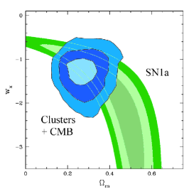
Figure 15: Left: $f_{B}$ measured for a sample of high–z clusters in an EdS cosmology (dots) and in a flat $\Lambda$ universe (empty diamonds, from Ettori et al. 2003). Right: constraints in the $w$–$\Omega_{0}$ plane obtained by combaining baryonic fraction in clusters and CMB (Allen et al. 2004).

3.3 Future prospects for precision cosmology with clusters

We are approaching the end of our brief introduction to cosmological tests with clusters of galaxies. A clear way to summarize it, is the cosmic triangle shown in Figure 16. Each side represents one of the three main parameters: the mass density, the cosmological constant, and the curvature. Contours levels perpendicular to one side mean that a particular test is efficient in constraining that parameter. Cosmological tests based on clusters are mostly sensitive to $\Omega_{0}$, while geometrical tests like CMB and SNeIa are more sensitive to the curvature and $\Omega_{\Lambda}$. Roughly speaking, CMB can constrain $\Omega_{0}+\Omega_{\Lambda}$, while SNeIa $\Omega_{0}-\Omega_{\Lambda}$, mainly beacuse of the different redshift range, 0.5–2 for SNeIa and  1000 for CMB. Obviously, the combination of the three tests is very powerful, but its application requires a good understanding of all the different systematics.

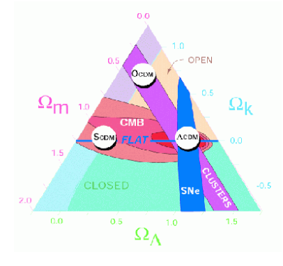
Figure 16: The cosmic triangle (Steinhardt 2003, see http://wwwphy.princeton.edu/ steinh/). The complementarity of the three classic cosmological tests is clearly shown.

This picture is still valid after recent observations by Chandra and XMM showed that the physics of clusters is more complicated than expected. The key questions on the future of precision cosmology with clusters of galaxies are: do we need a new, large, all–sky survey of clusters? Or should we first understand better the physics of the ICM? Therefore, which is the best instrument we should build next? I think that the best answer is that a new, medium–depth all–sky survey of clusters is needed for both aspects. First, a large survey can help in obtaining strong constraints on the cosmological parameters, providing at the same time large samples to investigate the relationship between X–ray observables and the dynamical masses. A second crucial aspect, is that a large survey would discover new clusters, especially at high redshift. This is mandatory to provide targets for the future X–ray missions, which will provide sensitive, narrow–field instruments to investigate the physics of the ICM. Without a new wide survey, we will run out of clusters to observe! Several proposals of medium–size mission have been circulated so far, but at present there are no planned large–area surveys of the X–ray sky. The future of X–ray cluster astrophysics largely depends on this.

4 What to bring home

At the end of this introduction, we should be aware that clusters of galaxies constitute a cosmological tools to significantly constrain $\Omega_{0}$ and the spectrum of primordial fluctuations, through tests based on dynamics or on geometry. X–ray observations offer the best tool to measure mass and collect complete sample of clusters. Main results points towards a flat $\Lambda$–dominated Universe ($\Omega\sim 0.3$ and $\Omega_{\Lambda}\sim 0.7$, or $w=-1$) and a normalization of the fluctuations power spectrum consistent with that measured from CMB for a CDM Universe ($\sigma_{8}\simeq 0.8$).

If someone wants to start the business of cosmological tests with clusters, she/he just needs basic programming skills to put in a simple code all the formulae we discussed, and a good X–ray observer among the collaborators, in order to have access to a well defined, complete survey of clusters. However, one must know that this game was played a lot starting from the 90’s, when it was realized that clusters constitute one of the most powerful cosmological tools. At present, in 2006, most of the best X–ray clusters surveys have been exploited in this sense. Therefore, if you want to start the business, you better have something smart in mind, mainly a way to deal with any possible systematics or with a better treatment of the effects of the poorly known thermodynamics of the ICM.

However, a noticeable contribution would be given by supporting the scientific case of future X–ray missions to obtain new data, in the form of a wide and complete sample of clusters. Larger samples indeed, will allow to study at the same time the thermodynamics of the ICM and the evolution of clusters as a population. Finally, one should not have the feeling that the physics of the ICM is now the hot topic at the expenses of precision cosmology, which should rely only on tests based on SNeIa and CMB. As a general comment, I would like to stress that clusters are probing a different cosmic epoch with respect to CMB, and a different physics with respect to SNeIa, therefore they will always be a complementary and useful test for cosmology. The complex ICM physics, insted of being an obstacle, must be seen as a further oppurtunity to learn about structure formation in the Universe.

References

- (1) Abell, G. O. 1958, ApJS, 3, 211
- (2) Allen, et al. 2004, MNRAS, 353, 457
- (3) Birkinshaw, M., & Lancaster, K., 2004, Proceedings of the International School of Physics ”Enrico Fermi”, Eds. Melchiorri, F. & Rephaeli, Y., astro-ph/0410336
- (4) Borgani, S., et al. 1999, ApJ, 517, 40
- (5) Borgani, S., et al. 2001, ApJ, 561, 13
- (6) Borgani, S., & Guzzo, L. 2001, Nature, 409, 39
- (7) Borgani, S., et al. 2004, MNRAS, 348, 1078
- (8) Bower, R.G. 1991, MNRAS, 248, 332
- (9) Broadhurst, T., et al. 2005, ApJ, 621, 53
- (10) Caldwell, R. R.; Dave, R., & Steinhardt, P.J. 1998, PhRvL, 80, 1582
- (11) Carlstrom et al. 2002, ARA&A, 40, 643
- (12) Cavaliere, A., & Fusco-Femiano, R. 1976, A&A, 49, 137
- (13) Dahle, H., et al. 2003, ApJ, 591, 662
- (14) Donahue, M., & Voit, G.M. 1999, ApJL, 523, 137
- (15) Eke, V.R., Navarro, J.F., Frenk, & C.S. 1998, ApJ, 503, 569
- (16) Ettori, S.,et al. 2003, A&A, 398, 879
- (17) Ettori, S.,et al. 2004, A&A, 417, 13
- (18) Fabian, A.C., et al. 2002, MNRAS, 331, 369
- (19) Fabian, A.C., et al. 2003, MNRAS, 344L, 43
- (20) Gal, R.R. 2006, Guillermo Haro Summer School, astro-ph/0601195
- (21) Gioia, I.M., et al. 1990, ApJL, 356, 35
- (22) Gladders, M.D., & Yee, H.K.C. 2005, ApJS, 157, 1
- (23) Hallman, E.J., et al. 2005, ApJ submitted, astro-ph/0509460
- (24) Holder, G.P., Carlstrom, J.E. 2001, ApJ, 558, 515
- (25) Ikebe, Y., et al. 2002, A&A, 383, 773
- (26) Jenkins, A., et al. 2001, MNRAS, 321, 372
- (27) Kaiser, N. 1986, MNRAS, 222, 323
- (28) Kaiser, N., 2002, Elements of Astrophysics, http://www.ifa.hawaii.edu/k̃aiser/
- (29) Kolb, E.W., & Turner, M.T. 1990, The Early Universe, Frontiers in Physics, v. 69, Addison–Wesley
- (30) Lacey, C., & Cole, S. 1993, MNRAS, 262, 627
- (31) Lahav, O., & Lidlle, A.R. 2006, in The Review of Particle Physics 2006, astro-ph/0601168
- (32) Mazzotta, P. et al. 2001, ApJ, 555, 205
- (33) Markevitch, M. et al. 2000, ApJ, 541, 542
- (34) Markevitch, M. et al. 2004, ApJ, 606, 819
- (35) Mo, H.J., & White, S.D.M. 1996, MNRAS, 282, 347
- (36) Peebles, P.J.E. 1993, Physical Cosmology (Princeton: Princeton Univ. Press)
- (37) Perlmutter, S., et al. 1999, ApJ, 517, 565
- (38) Peterson, J.R., & Fabian, A.C. 2005, Physics Reports, astro-ph/0512549
- (39) Pierpaoli, E., Scott, D., & White, M. 2001, MNRAS, 325, 77
- (40) Pierpaoli, E., et al. 2003, MNRAS, 342, 163
- (41) Ponman, T. J., Cannon, D. B., & Navarro, J.F. 1999, Nature, 397, 135
- (42) Press, W. H., & Schechter, P. 1974, ApJ, 187, 425
- (43) Ribicky, G.B., & Lighman, A.P. 1979, Radiative Processes in Astrophysics, Wiley & Sons Eds.
- (44) Rosati, P., et al. 1998, ApJL, 492, 21
- (45) Rosati, P., Borgani, S., & Norman, C. 2002, ARA&A, 40, 539
- (46) Rosati, P., et al. 2004, AJ, 127, 230
- (47) Sarazin, C.L. 1988, X–ray Emission from Clusters of Galaxies, (Cambridge: Cambridge University Press)
- (48) Schuecker, P., et al. 2003, A&A, 402, 53
- (49) Spergel, D.N., et al. 2003, ApJS, 148, 175
- (50) Springel, D.N., at al., 2005, Nature, 435, 629
- (51) Sunyaev, R. A., & Zeldovich, Ya. B. 1972, CoASP, 4, 173
- (52) Steinhardt, 2003, http://wwwphy.princeton.edu/steinh/
- (53) Tegmark, M. 2002, http://space.mit.edu/home/tegmark/sdss.html
- (54) Tozzi, P., & Norman, C. 2001, ApJ, 546, 63
- (55) Vikhlinin, A. et al. 2001, ApJ, 551, 160
- (56) Vikhlinin, A. et al. 2002, ApJ, 578, 107
- (57) Vikhlinin, A. et al. 2005, ApJ, 628, 655
- (58) Voit, G.M., Kay, S.T., & Bryan, G.L. 2005, MNRAS, 364, 909
- (59) White, S.D.M., et al. 1993, Nature, 366, 429