Ultraviolet–to–Far–Infrared Properties of Local Star–Forming Galaxies

Abstract

We present the results of a multiwavelength study of nearby galaxies, aimed at understanding the relation between the ultraviolet and far–infrared emission in star–forming galaxies. The dataset comprises new ultraviolet (from HST/STIS), ground–based H$\alpha$, and radio continuum observations, together with archival infrared data (from IRAS and ISO). The local galaxies are used as benchmarks for comparison of the infrared–to–ultraviolet properties with two populations of high–redshift galaxies: the sub–millimeter star–forming galaxies detected by SCUBA and the ultraviolet–selected Lyman Break galaxies. In addition, the long wavelength baseline covered by the present data enables us to compare the star formation rates (SFRs) derived from the observed ultraviolet, H$\alpha$, infrared, and radio luminosities, and to gauge the impact of dust opacity in the local galaxies. We also derive a new calibration for the non-thermal part of the radio SFR estimator, based on the comparison of 1.4 GHz measurements with a new estimator of the bolometric luminosity of the star forming regions. We find that more actively star forming galaxies show higher dust opacities, in line with previous results. We find that the local star–forming galaxies have lower F_λ(205 $\mu$m)/F_λ(UV) ratio, by two–three orders of magnitude than the submillimeter–selected galaxies, and may have similar or somewhat higher F_λ(205 $\mu$m)/F_λ(UV) than Lyman Break Galaxies. The F_λ(205 $\mu$m)/F_λ(UV) ratio of the local galaxy population may be influenced by the cool dust emission in the far–infrared heated by non-ionizing stellar populations, which may be reduced or absent in the LBGs.

1 Introduction

The presence of observational and/or physical links between local star–forming galaxies and high–redshift ultraviolet–selected and infrared–selected galaxies is still subject of scrutiny, in view of their importance for placing the high–redshift populations in the context of galaxy evolution. One of the outstanding questions is how the observed UV (restframe $\sim$1600 Å) and far–infrared (restframe 200–260 $\mu$m) properties of the high–redshift populations relate to the analogous properties of local star–forming galaxies.

In galaxies, the restframe UV emission traces massive stars and the recent star formation, modulo the effects of dust opacity. The far infrared emission at 200–260 $\mu$m traces the Rayleigh–Jeans tail of the dust emission. Evolved stellar populations unassociated with the recent star formation may heat the dust to relatively cool temperatures (T$\lesssim$20 K, e.g. Helou 1986; Lonsdale-Persson & Helou 1987; Rowan-Robinson & Crawford 1989; Rowan-Robinson & Efstathiou 1993), which can provide a significant contribution to the emission at the long wavelengths. The relevance of investigating F_λ(200–260 $\mu$m) comes from the discovery in recent years of a significant population of submillimeter–bright sources at high redshifts observed with SCUBA (Chapman et al. 2003, 2005; Wang, Cowie, & Barger 2004; Aretxaga, Hughes, & Dunlop 2005; Smail et al. 1997; Barger et al. 1998, 2000; Blain et al. 1999a,b). SCUBA is most sensitive at 850 $\mu$m, which corresponds to restframe 210–260$\mu$m at redshift z$\sim$2.2–3.

The ultraviolet–selected Lyman Break galaxies at z$\sim$3 (LBGs, Steidel et al. 1999) resemble local UV–bright starburst galaxies in many of their UV spectral properties (Meurer, Heckman, & Calzetti 1999; Adelberger, & Steidel 2000). The LBGs have been argued to be the major contributor of the global star formation at redshift $\sim$2–4 (Adelberger & Steidel 2000, Giavalisco 2002; Giavalisco et al. 2004), although this has been recently challenged by Chapman et al.(2005). Chapman et al. (2005) have suggested that the sub–millimeter–detected galaxies at high redshift (SCUBA sources, median z$\sim$2.2) represent a distinct and complementary population to the LBGs; the authors also argue that this population provides a significant contribution to the SFR density of the Universe in the redshift range z$\sim$2–3.

The sub-mm selected sources have been linked to local Ultra Luminous Infrared Galaxies (ULIGs, Smail et al. 1997; Blain et al. 1999a,b), with star formation rates per unit area close to the ’maximum starburst limit’ of Lehnert & Heckman (1996), Meurer et al. (1997) and total rates of many 100’s M_⊙ yr^-1 (Barger et al. 1998; Chapman et al. 2004, 2005; Hughes et al. 1998). Like ULIGs, SCUBA sources tend to be faint in the restframe ultraviolet (Chapman et al. 2005), but unlike ULIGs, many SCUBA sources show evidence of extended star formation over many kpc (Chapman et al. 2004).

Conversely, the z$\sim$3 LBGs are faint, typically undetected, in the SCUBA waveband, with fluxes around or below the 1 mJy level (Chapman et al. 2000). As previously suggested (Chapman et al. 2005, and references therein), the LBGs and the SCUBA sources likely represent complementary facets of the high–redshift star formation: UV–bright and 210 $\mu$m–faint the first, and UV–faint and 210–260 $\mu$m–bright the second, perhaps marking a continuum of properties similar to that in the local Universe between UV–bright starbursts and ULIGs.

Relating these characteristics to those of local populations has proceeded so far in a piecemeal fashion with small samples of nearby galaxies observed simultaneously in the UV and the restframe $\sim$200 $\mu$m. For this reason we obtained HST/STIS–UV (1600Å) observations of a sample of local star–forming galaxies for which archival ISO observations at $\lambda>$170 $\mu$m existed. The sample is large enough to offer a unique opportunity to compare the UV/FIR properties of local galaxies with those of observations in similar wavebands of high–redshift galaxies.

The availability of an homogeneous set of new ultraviolet, H$\alpha$ and radio data, augmented with IRAS/ISO infrared data, enables us also to investigate the impact of dust opacity on UV and optical SFR indicators. There are extensive studies on the subject performed on a variety of samples of local galaxies (e.g., Sullivan et al. 2001, Kewley et al. 2002, 2004, Rosa González et al. 2002, Hopkins et al. 2003, Bell 2003). Kewley et al. (2002, 2004) uses SFR(IR) as a benchmark for analyzing SFR(H$\alpha$) and SFR([OII]) for galaxies in the Nearby Field Galaxy Survey. A similar approach is used by Rosa González et al. (2002), while Hopkins et al. (2003) use SFR(1.4 GHz) as a reference to investigate optical SFR estimators for the galaxies of the Sloan Digital Sky Survey. A similar study to ours has been undertaken by Bell (2003), using however a less homogeneous dataset. A major study on the cross–correlation of multiwavelength SFR estimators is being undertaken by the SINGS project (the Spitzer Infrared Nearby Galaxies Survey, Kennicutt et al. 2003), that will combine data from the B-band through the near-IR, mid-IR and far-IR (up to 160$\mu$m), all the way to the radio; SINGS will provide a complete, homogeneous dataset for this type of investigation. The present study is at the same time complementary to and independent of SINGS, as there is minimal overlap between the galaxy samples (only three objects in common). We derive a new calibration for SFR(radio), based on the comparison of this indicator with a new indicator of the bolometric luminosity of the star forming regions, which represents a better approximation of the actual bolometric luminosity than simply using the infrared luminosity. These results are compared with other empirically derived calibrations based on the radio–FIR correlation (Yun et al. 2001, Bell 2003).

This paper is organized in the following way. In Section 2 we present the data and sample being used. In Section 3 we present the star formation rate calibrations employed. A comparison between the different SFRs is given in Section 4, where we also present an improved radio SFR calibration. Section 5 presents the IR/UV properties of the sample and compares it to high-redshift galaxies. A summary of the results is given in Section 6. We assume H${}_{o}=75$ km s^-1 Mpc^-1 throughout this paper, and, where necessary, convert data from other papers to this value.

2 The Data

2.1 Nearby Galaxies

The data and measurements of nearby star forming galaxies used in the current paper are presented in Paper I (Schmitt et al. 2005). Our sample consists of 41 galaxies spanning a wide range in the intrinsic parameters of luminosity, star formation rate and metallicity. We point out that these galaxies were culled from the ISO archive, so the sample may still have some selection effects and may not necessarily represent typical galaxies, like a volume limited sample. Measurements were made in the UV (1600Å) with HST/STIS, in H$\alpha$ with ground-based facilities and HST archival data, and in the radio at 8.46 GHz, 4.89 GHz and 1.4 GHz (3.6 cm, 6 cm and 20 cm, respectively), with the VLA and literature data. Archival IRAS and ISO data were utilized for the infrared; 29 out of 41 galaxies presented here have ISO data at wavelengths longward of 170 $\mu$m (Schmitt et al. 2005), thus providing a direct comparison with SCUBA data for objects at redshift z$\sim$2-3. More details about the data reductions, measurements and characteristics are given in Paper I. The UV data were obtained with an aperture that is about 25″ in side, which is smaller than the typical size of our galaxies. In the present paper we will only compare UV data with H$\alpha$ and radio 8.46 GHz data measured inside an aperture that matches the UV one. The infrared data encompass the entire galaxy, and care will be taken when comparing these measurements to those at other wavelengths, so as to mitigate the effects of aperture mismatch.

In the case of UV, H$\alpha$ and radio data we simply use the monochromatic luminosities to convert to star formation rates, as detailed in the next section. In the case of the infrared emission we integrate the area under the spectral energy distribution between 8$\mu$m and 1 mm to derive star formation rates. This is accomplished by fitting two temperature models to the data of those galaxies (see Table 5 in paper I) that had at least one measurement from ISO longward of 100$\mu$m. We assumed that the dust emissivity has index $\epsilon=2$. We present in Figure 1 the example of three of these fits. The agreement between the fit and observed points is usually very good. Fitting two temperature models with fixed emissivity $\epsilon$ allows more flexible SEDs than a single temperature with variable $\epsilon$, since in the former case two maxima are one of the possible solutions (e.g. NGC 3079 Figure 1). In the case of NGC 4088 and NGC 6217 it was necessary to eliminate the 170$\mu$m measurements, which were clearly discrepant and probably had calibration problems, and only retain longer wavelength measurements (180$\mu$m and higher ISO measurements). Only for one of the galaxies in the sample, NGC 5860, a one temperature model was the best fit to the infrared data (Calzetti et al. 2000).

The results of the fits to the far infrared data are presented in Table 1. This table gives the infrared fluxes, integrated between 8$\mu$m and 1 mm, obtained from these fits, as well as the values extrapolated based on IRAS measurements alone (F(IR) calculated using the expression from Sanders & Mirabel 1996). We also give the temperatures of the warm and cold components, as well as their fractional contribution to the far infrared flux.

The total infrared emission derived from our fits has been compared to the total infrared emission derived from the extrapolated IRAS measurements. In general we find that the discrepancy between the two numbers is relatively small, of the order of 25%, with a median ratio F(IR)/F_IRAS(IR)=0.94. Figure 2 shows that there is a clear trend between F(IR)/F_IRAS(IR) to increase for large F100/F60 (ratio between the IRAS 100$\mu$m and 60$\mu$m fluxes). The relation between the two quantities can be expressed by the linear fit

$$\log F(IR)/F_{IRAS}(IR)=-0.08\pm 0.01+(0.19\pm 0.04)\log F100/F60$$ (1)

Since F100/F60 is a temperature indicator, the above relation shows that the IRAS extrapolation overpredicts the infrared emission for warmer sources and underpredicts it for the cooler ones. This result is in line with those found by Dale et al. (2001), which indicates that the Sanders & Mirabel (1996) relation can give results that are up to $\sim$25% deviant. Dale et al. (2001) also point out that the ratio F60/F100 produces the tightest correlation with other infrared measurements, making it the ideal choice to parameterize the correction for F_IR(IRAS). We use equation (1) to correct the total infrared fluxes for the 12 galaxies ($\sim$29%  of the sample) for which IRAS but not ISO measurements are available.

2.2 ULIGs, LBGs and SCUBA Sources

In order to compare the local galaxies with their high redshift counterparts we retrieved data from the literature for Arp 220, another 4 ULIGS, 13 LBGs, and 31 SCUBA sources (the latter in the redshift range 2–3.5), for which both rest frame UV and rest frame $\sim 200\mu$m measurements were available.

For Arp 220 and the 4 ULIGs (IC 883, Mrk 273, IRAS 15250$+$3609 and IRAS 19254–7245) UV data was obtained from Goldader et al. (2002), while the 205$\mu$m and FIR data came from ISO and IRAS observations published by Klaas et al. (2001). We also obtained radio 6 cm data for Arp 220 (Becker, White & Edwards 1991). In the case of the LBGs, their UV emission is well known, from selection, but the majority of these sources are not detected in submm observations. Here we use the sample of LBGs from Chapman et al. (2000), which comprises 13 galaxies with z$\sim$3, observed at 850$\mu$m with SCUBA. Only one of these sources was detected (W-MMD 11), while the remaining ones had only upper limits. We assume that for these galaxies the upper limit of SFR(BOL_SB), the star formation rate calculated using the bolometric luminosity, is equal to the SFR(850$\mu$m) upper limit given by Chapman et al. (2000). We also assume the 1$\sigma$ r.m.s. value to be the 200$\mu$m upper limit.

A situation opposite to the LBGs happens for SCUBA sources, which are detected in the submm, but not always have optical counterparts or spectroscopic redshifts. Using the compilations from Chapman et al. (2003, 2005) we selected 31 SCUBA sources, from an initial sample of 73, with spectroscopic redshifts z$>2$. These 31 galaxies do not include sources classified as AGN (Aretxaga et al. 2005; Chapman et al. 2005), although we include one source with a composite AGN/Starburst characteristics. The measurements obtained from these papers are the broad band $\cal{R}_{AB}$ magnitudes, which were converted to rest frame UV fluxes, radio 20 cm measurements, as well as bolometric luminosities calculated fitting SEDs to the 850$\mu$m and radio fluxes (Chapman et al. 2003, 2005). These values are used to calculate SFR(BOL_SB), and L_λ(205$\mu$m)/L_λ(UV) (we define L_λ(205$\mu$m) as the restframe luminosity measured with SCUBA for uniformity with the other galaxy samples, although the restframe wavelength is in the range 210-260$\mu$m).

3 Calibrations of Star Formation Rates

The UV, H$\alpha$ and IR star formation rates were calculated using the calibrations presented by Kennicutt (1998):

$$SFR(H\alpha)=7.9\times 10^{-42}L(H\alpha) [erg~{}s^{-1}]$$ (2)

$$SFR(UV)=1.4\times 10^{-28}L_{\nu}(1600) [erg~{}s^{-1}~{}Hz^{-1}]$$ (3)

$$SFR(IR)=4.5\times 10^{-44}L(IR) [erg~{}s^{-1}]$$ (4)

Where all the SFRs are in solar masses per year calculated for a Salpeter IMF between 0.1 and 100 M_⊙. The UV and H$\alpha$ luminosities were corrected for foreground Galactic extinction, but not for internal extinction. The SFR(IR) is a correct estimator of the star formation rate in a galaxy only for large dust optical depths and young star dominated spectral energy distributions (Kennicutt 1998). In the case of the radio we followed the same approach used by Condon & Yin (1990) and Condon (1992) to derive a new calibration, described below.

First, we assume that the non-thermal radio emission from the Milky Way is entirely due to supernova remnants. This flux is L(408 MHz)$\sim 6\times 10^{21}$ W Hz^-1 (Berkhuijsen 1984) with a spectral index $\nu^{-0.8}$. For the supernova rate we use $\nu_{SN}\sim 0.023$yr^-1 (Tammann 1982; Tammann, Loeffler, & Schroeder 1994). This rate corresponds only to core collapse supernovae and was calculated assuming that the Milky Way is an Sc galaxy. Notice that the percentage of core-collapse to Type Ia supernovae would decrease by a factor of $\sim$10% if the Milky Way was assumed to be an Sb galaxy. These numbers also carry some uncertainties due to biases in the detection of supernovae and the corrections that are applied in the determination of supernova rates (Cappellaro et al. 1997; Cappellaro, Evans, & Turatto 1999; and references therein). Type Ia supernovae are not taken into account in the SFR calculations because they are traditionally related to the old stellar population. However, recent results suggest that this may not be true (Mannucci et al. 2005; Scannapieco & Bildsten 2005), which may require a future revision of this calibration.

Following these assumptions, the non-thermal radio luminosity due to supernovae can be calculated from $L_{\nu}(N)\sim 1.3\times 10^{23}\nu^{-0.8}\nu_{SN}$, in units of W Hz^-1, the frequency ($\nu$) is in units of GHz and the supernova rate ($\nu_{SN}$) in units of yr^-1. The conversion between this value and the star formation rate is done in the same way Kennicutt (1998) derived the IR calibration. Using a Starburst 99 (Leitherer et al. 1999) model for a galaxy with continuous star formation rate of 1 M_⊙ yr^-1, with a Salpeter IMF, solar metallicity, lower and upper mass cutoff 1 and 100 M_⊙, respectively, we find that the average supernova rate reaches an asymptotic value of $\nu_{SN}\sim 0.0168$yr^-1 around 100 Myr. Converting the star formation rate to a lower mass cutoff of 0.1 M_⊙ and using the above relation between non-thermal radio emission and the supernova rate, we get:

$$L_{\nu}(N)\sim 8.55\times 10^{20}\nu^{-0.8}SFR$$ (5)

where SFR is the rate of stars in the mass range 0.1-100 M_⊙ being formed, in units of M_⊙ yr^-1, $\nu$ is the frequency of the radio observations, in GHz, and L${}_{\nu}(N)$ is the non-thermal radio luminosity at this frequency, in units of W Hz^-1.

The contribution from thermal emission to the radio continuum is taken from Condon (1992), where we used the new H$\alpha$ to SFR conversion by Kennicutt (1998), thus extending the lower mass cutoff of the stellar IMF to 0.1 M_⊙.

$$L_{\nu}(T)\sim 1.6\times 10^{20}\nu^{-0.1}SFR$$ (6)

The total SFR at radio wavelengths is therefore calculated by simply summing up the appropriate thermal and non-thermal contributions at a given frequency

$$SFR(RADIO)=L_{\nu}\times 10^{-20}/(8.55\nu^{-0.8}+1.6\nu^{-0.1})[WHz^{-1}]$$ (7)

which at 1.4 GHz corresponds to SFR$=1.24\times 10^{-21}$ L_ν(1.4 GHz). Notice that, although the radio emission has the advantage of being independent of reddening, it is not as direct a tracer of star formation as UV and H$\alpha$, given the assumptions included in the derivation of the non–thermal portion.

Finally, we also define a new multiwavelength SFR indicator, by combining the emission from the UV, B and IR bands, which we call SFR(BOL_SB). This quantity is calculated by integrating the SED between the UV and B part of the spectrum, and adding this quantity to L_IR. The specifier BOL_SB refers to the fact that we are essentially computing the bolometric luminosity of the starburst, as these blue bands are dominated by the emission from the young massive stars of the starburst itself (the B band data of the galaxies in the sample is listed in Paper I). This is particularly important for a sample that spans a wide range of luminosities, as the less luminous objects tend to be less dust opaque and thus to have a higher fraction of the stellar light coming out directly in the UV and B. The corresponding SFRs are calculated using the IR calibration from Kennicutt (1998). This is an extension of the SFR(UV$+$IR) introduced by Wang & Heckman (1996) and Heckman et al. (1998) for normal star–forming and starburst galaxies, respectively. BOL_SB is a more accurate estimator of SFR than L_IR, since in our galaxies a non–negligible fraction of the stellar light emerges directly in the UV and B bands, unabsorbed by dust; hence L_IR alone is not a good approximation to the bolometric luminosity, especially for the less bright and less dusty galaxies. Incidentally, although SFR(BOL_SB) also includes the B band flux, it generally gives values that are on average very similar to SFR(UV$+$IR), with a spread smaller than 10% around the median.

4 Comparison of Star Formation Rates

4.1 Matched Apertures

Given the small aperture with which the UV data were obtained, we compare their SFRs only with H$\alpha$ and radio (8.4 GHz) ones measured inside a matching aperture. In Figure 3 we show the ratios SFR(H$\alpha$)/SFR(UV) (top panel) and SFR(UV)/SFR(8.4 GHz) (bottom left panel) as a function of SFR(8.4 GHz). In both cases the SFR derived from UV is lower than the one derived from the other indicator, clearly showing the effects of extinction. Of particular interest is the large scatter in the SFR(UV)/SFR(8.4 GHz) plot, which clearly shows that dust extinction has a strong effect on measurements of SFR at short wavelengths. A similar result is seen in the SFR(H$\alpha$)/SFR(8.4 GHz) plot (bottom left panel). This highlights the importance of extinction corrections, since in some cases the uncorrected UV and H$\alpha$ measurements can underpredict the SFR by a factor as high as 100. Nevertheless, the SFR(H$\alpha$)/SFR(UV) ratio remains strongly correlated, suggesting that both wavebands probe comparably low extinction regions. We stress the importance of subtracting the [NII] contribution from the flux in H$\alpha$ images, as [NII] contamination becomes increasingly important in high metallicity systems (Storchi-Bergmann, Calzetti, & Kinney 1994), where the [NII] emission can contribute to as much as half of the total flux.

4.2 Integrated Apertures

Emission integrated over the entire body of the galaxies is available at H$\alpha$, IR, and radio wavelengths. Here we compare global SFRs among the different wavebands (Figure 4). We generally find a good agreement between the different indicators, with a few deviations. In the case of H$\alpha$, the SFR usually is underestimated because of dust extinction. We find that the amount of extinction increases for high luminosity sources. This result represents an independent confirmation of those from Wang & Heckman (1996), Heckman et al. (1998), Sullivan et al. (2001), Martin et al. (2005) who find a tred for more opaque galaxies to have higher star formation rates (see Section 5 for further discussion on this subject). Figure 4 gives further support to this interpretation, where we can see that using uncorrected H$\alpha$ fluxes can underestimate the star formation rate by a factor of 10 or larger in the most luminous sources. This result agrees with those from Cram et al. (1998), Sullivan et al. (2001) and Afonso et al. (2003).

Another noticeable deviation is found in the comparison of SFRs in different radio wavelengths, where we can see that the 8.4 GHz generally gives lower values than 1.4 GHz. We believe that this is due to limitations of our observations, since the 8.4 GHz images had a beamsize of $\sim$3″ and maximum field of view of 180″, thus missing some of the faint diffuse 8.4 GHz emission in the more extended sources. This was not an issue for the 1.4 GHz measurements.

4.3 New Radio SFR calibration

One of the most important results obtained from the comparison of the integrated star formation indicators is shows in the top panels of Figure 5. This Figure shows the discrepancy between SFR(BOL_SB) and SFR(Radio), both 4.89 GHz and 1.4 GHz, in the sense that the values determined from radio measurements tends to be higher than the ones obtained from the bolometric luminosity by a factor of $\sim$2. This difference is similar to the one found by Condon, Cotton & Broderick (2002), and Bell (2003).

This disagreement could be the result of an overestimation of the radio relation, or to an underestimation of the BOL_SB (infrared) relation. Taking into account the fact that the infrared SFR relation is a more direct calibration than the radio one, and that it has been tested against calibrations at other wavebands (e.g. Kewley et al. 2004, Rosa-González et al. 2002), we attribute the observed disagreement to the radio calibration. Notice however, that an opposite result was presented by Cappellaro et al. (1999), who found that the Far-Infrared luminosity does not correlate with supernova rates in nearby galaxies. Although this result seems to indicate that infrared is not a universal measurement of SFR, their measurements were biased towards normal low luminosity quiescent galaxies, and cannot be considered representative of the sources studied in this paper. Furthermore, since we used BOL_SB instead of L(IR), we removed most of systematic effects in the infrared calibration.

Here we propose a correction to the radio SFR relation, based on the comparison between the 1.4 GHz and BOL_SB results. We find that the median ratio SFR(BOL_SB)/SFR(1.4 GHz) is 0.48, which gives us the corrected SFR(1.4 GHz) relation,

$$SFR=6.2\times 10^{-22}L_{\nu}(1.4GHz)[WHz^{-1}]$$ (8)

A comparison between this new relation and the one from Yun, Reddy & Condon (2001), who derived SFR(1.4 GHz) based on the comparison between the integrated radio and infrared luminosity functions, shows a good agreement. We also find a good agreement when comparing our result with the one from Bell (2003). However, given the luminosity range of our galaxies we are not able to see the deviation from linearity seen by Bell (2003) in the low luminosity range. Using the SFR(IR) calibration from Kennicutt (1998) and the radio-FIR correlation given by Yun et al. (2001) we get an SFR(1.4 GHz) relation in agreement with equation 8 within an uncertainty of 20%. The uncertainty is mostly driven by the assumption used to convert L(40-120$\mu$m) to L(IR). A variation of about 20% is typical of what is found in galaxies (Dale et al. 2001).

Next we determine a new relation for the non-thermal part of the radio SFR calibration (Equation 5). Since the non-thermal part of the relation is based on indirect assumptions, which depend mainly on the supernova rate of the Galaxy and their average non-thermal flux, it is subject to large uncertainties. For instance, Condon (1992) pointed out the discrepancy between the predicted and observed supernova rate of the Galaxy. Another potential problem is that the measured 408 MHz flux of the Milky Way carries large uncertainties. Conversely, we assume that the uncertainties in the thermal part of the calibration (Equation 6) are insignificant when compared to the non-thermal ones, since that relation is derived directly from SFR(H$\alpha$) (Kennicutt 1998), which has been tested against other calibrations. Using Equations 6 and 8 we find the following non-thermal radio SFR relation:

$$L_{\nu}(N)\sim 1.92\times 10^{21}\nu^{-0.8}SFR$$ (9)

Using Equations 6 and 9 we can calculate the radio SFR relations at 4.89 GHz and 8.46 GHz, given below:

$$SFR=1.4\times 10^{-21}L_{\nu}(4.89GHz) [WHz^{-1}]$$ (10)

$$SFR=2.0\times 10^{-21}L_{\nu}(8.46GHz) [WHz^{-1}]$$ (11)

A comparison between the new SFR(4.89 GHz) and SFR(1.4 GHz) with values obtained from BOL_SB (Figure 5 bottom panels) shows a very good agreement, indicating that the new radio relations are indeed more appropriate for the calculation of SFRs. We do not find as good an agreement for 8.46 GHz, but this is related to observational issues described above. It should also be noticed that Equation 10 has a direct application to high-redshift galaxies, where 20 cm observations correspond to restframe 6-7 cm for a z$\sim$3 object.

4.4 Extinction and other Effects Influencing SFRs

The effects of extinction suggested by Figure 3 are quantified in Figure 6. This figure shows the color excess E(B-V) derived from each pair of wavebands in Figure 3, requiring that any deviation of the SFR ratios from unity is due to dust extinction. In the case of SFR(8.4 GHz) we use the new calibration described above. For the UV, the color excess is derived using the reddening curve of Calzetti et al. (2000). We find that the different E(B-V) estimates have similar medians, albeit with a wide range of values, implying that dust geometry has a secondary impact (beyond that described by Calzetti 2001) on the SFR measurements at different wavelengths for our galaxy sample. A comparison of E(B-V) values calculated using UV/8.4 GHz and H$\alpha$/8.4 GHz, for galaxies with measurements available in the 3 wavebands, show that they are correlated. This indicates that the SFR differences relative to SFR(8.4 GHz) are due to dust extiction. It is also worth recalling here that although E(B-V)${}_{UV}\sim$E(B-V)_Hα, the resulting A${}_{UV}\sim 2.3$ mag$>$A${}_{H\alpha}\sim 1.5$ mag, thus explaining the trend in Figure 3.

Another important result of Figure 6 is the large spread of the extinction corrections among the galaxies in our sample, which have an interquartile range of the order of 0.5 mag. This indicates that assuming a single extinction value may work only on a statistical sense, for large samples of galaxies with similar characteristics. More detailed studies of this issue were performed by Bell & Kennicutt (2001), Rosa-Gonzalez, Terlevich, & Terlevich (2002), and Afonso et al. (2003).

Our SFR estimates are based on the assumption that we can use one conversion from flux to SFR for all galaxies. Clearly, this will be valid only in first order, as galaxy–to–galaxy variations of the stellar Initial Mass Function (IMF), metallicity (Leitherer et al. 1999), and star formation history (Sullivan, et al. 2004), in addition to dust absorption of Lyman continuum photons before reprocessing into H$\alpha$ light (Inoue 2001), and simplistic assumptions about the conditions of nebular recombination (e.g. Charlot & Longhetti 2001), will all affect SFR measurements. Indeed, we believe these potential galaxy–to–galaxy variations to contribute, together with dust geometry variations, to the scatter in the data observed in Figures 3 to 6.

As an example, we will discuss the impact of stellar IMF variations. The part of the IMF of concern here is the high end, as massive stars are those contributing to the UV emission and to the gas ionization. From Leitherer et al. (1999), a stellar population with a M_up=30 M_⊙ Salpeter IMF produces about 5 times less ionizing photons and about twice less UV continuum flux than a stellar population with a M_up=100 M_⊙ Salpeter IMF. Thus, SFR(UV)/SFR(H$\alpha$) calculated for the two populations will differ by about a factor of 2.5, without having to invoke any other effect (e.g., dust geometry variations). SFR(radio) closely follows the variation of SFR(H$\alpha$), being due to similar stars. If interpreted as a difference due to dust, it would correspond to E(B$-$V)$\sim$0.5 mag, roughly the range of our scatter (Figure 6, top panel). We note that this should be considered an extreme scenario, since Elmegreen (2005, Cambridge Prooceedings) has collected evidence that IMF variations are likely to be relatively small from galaxy to galaxy, and from environment to environment. Metallicity variations introduce even smaller effects than IMF variations on the multiwavelength SFR determinations (Leitherer et al. 1999).

5 Comparison of the UV/IR Properties of Nearby and High-Redshift Galaxies

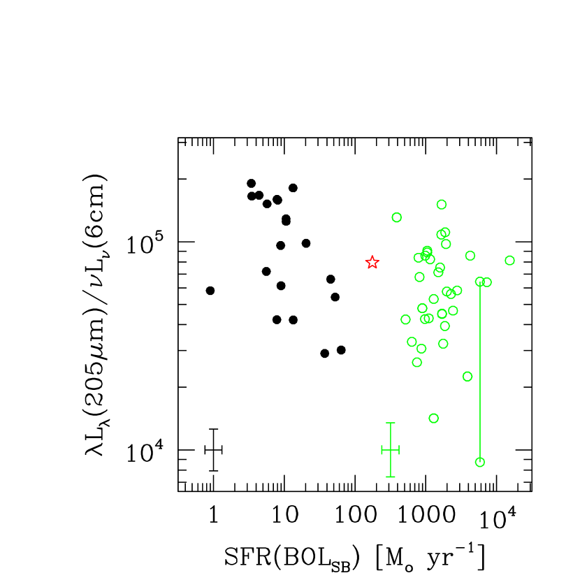
Figure 7: The left panel shows the radio 1.4 GHz$\times$FIR diagram for our galaxies, with the relation from Condon et al. (1991) shown as a solid line (median errorbar is shown in the top left corner). The right panel shows the infrared L_λ(205$\mu$m) over radio L_ν(6 cm) flux density ratio as a function of star formation rate. The filled dots represent our data points, the red star represents Arp 220 and the open green circles represent SCUBA sources. One of the SCUBA sources (SMM J 163650.0$+$405733) has two radio fluxes related to it (Ivison et al. 2002), as described in the text, so we show the two values connected by a vertical bar. The black errorbar (bottom left) shows the median error for our sample, and the green one (bottom middle) corresponds to the median error of the SCUBA sources.

As a first test, to see if there is any systematic difference between our galaxies and the general population of nearby sources, we show in the left panel of Figure 7 the plot of radio 1.4 GHz $\times$ FIR (FIR is calculated as described in Sanders & Mirabel 1996, using only the 60 and 100$\mu$m fluxes). A comparison between the relation obtained by Condon, Anderson & Helou (1991), solid line, and the values measured for our galaxies show a very good agreement, indicating that our sample is representative of the population of nearby star–forming galaxies.

Another test performed with the data was to check if there is any difference between the nearby galaxies and the SCUBA sources (Figure 7 right panel). This was done by comparing the ratio of monochromatic IR to radio (6 cm) emission of our galaxies, Arp 220 and the SCUBA sources from Chapman et al. (2003, 2005). We chose this radio frequency because it corresponds to observed $\sim$20 cm at z$\sim$2.2, the median redshift of the SCUBA galaxies, and is the frequency at which most of the deep radio surveys are done. Given the uncertainty in the slopes of the radio spectrum of these sources we do not try to apply any correction to the data, to put all the measurements in the same rest frame frequency. This figure shows that there is no strong correlation between L_λ(205$\mu$m)/L_ν(6 cm) and SFR(BOL_SB), apart from a small decrease in the ratio for higher SFRs (higher IR luminosity). This is an expected result, in line with those from Condon et al. (1991), thus confirming that there are no problems with the sample. According to Yun, Reddy & Condon (2001), this slope as a function of luminosity is due to the contribution from the general field populations to the far-infrared emission in quiescently star–forming galaxies.

The star–forming galaxies in our sample show the same range in IR$+$UV luminosity properties as those shown by the starburst galaxies analyzed by Heckman et al. (1998). In particular, there is a trend for more luminous galaxies to have a higher IR/UV luminosity ratio (Figure 8), indicating that more actively star–forming galaxies also tend to be more dust opaque, a trend already noted in other samples (Wang & Heckman 1996, Heckman et al. 1998, Sullivan et al. 2001, Hopkins et al. 2001; Martin et al. 2005). We compare in Figure 8 the best fitting relation obtained from our data (dotted line) with the one obtained when fitting the starbursts data from Heckman et al. (1998), using L(IR)$+\lambda$L_λ(UV) as independent variable (solid line). We can see that both samples produce very similar fits, which also is consistent with the trend seen in the UV selected star forming galaxies from Martin et al. (2005), given the large uncertainties in our sample and the different choice of IR luminosities in the Martin et al. (2005). The only difference is that our galaxies at the bright end tend to have on average slightly lower, by a factor of a few, L(IR)/L_λ(UV) ratio at the same total IR$+$UV luminosity. This difference can be explained if not all the observed UV emission is associated with current star formation, as observed in NGC5194 (Calzetti et al. 2005), and/or if the starburst dust geometry is not readily applicable to star–forming galaxies; both effects can boost the UV emission relative to the infrared (Calzetti 2001, Buat et al. 2002). As far as SFR(BOL_SB) is concerned, the impact on this value of the UV emission unrelated to current star formation will be minimal as L_IR provides most of the bolometric light for our brightest normal star forming galaxies.

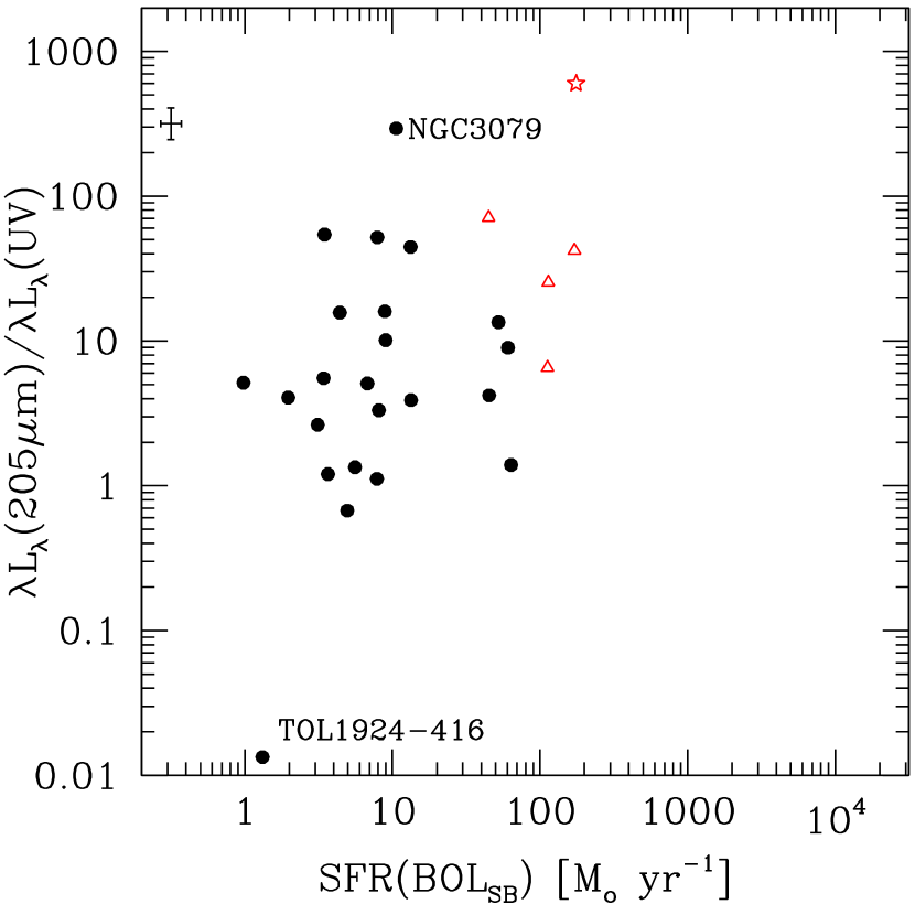
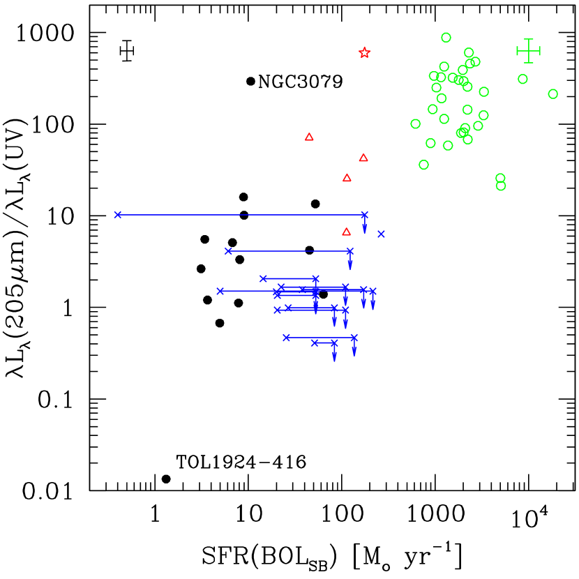
Figure 9: The monochromatic IR flux to UV ratio as a function of the bolometric star formation rate for all galaxies in our sample (left) and only those galaxies for which more than 50% of the radio emission is contained within the STIS aperture (right). Filled dots represent our data points, the red star is Arp 220, the red triangles are ULIGs (Goldader et al. 2002; Klaas et al. 2001; Becker et al. 1991), green open circles represent SCUBA sources (Chapman et al. 2003, 2005) and crosses represent LBGs (Chapman et al. 2000). The black point with small $\lambda$L_λ(205$\mu$m)/$\lambda$L_λ(UV) corresponds to TOL 1924–416, which is a dwarf galaxy with a young starburst and almost no emission from cold dust, while the point with the largest ratio is NGC 3079, a high inclination galaxy known to harbor an AGN. In the case of LBGs, with the exception of one source, they are all upper limits on the Y axis. Along the X axis the LBG’s have SFR’s that are bracketed by the upper limits from SFR(210$\mu$m) and the lower limits given by the observed UV. The median errorbar of our sample is shown in black in the top left corner, while in the case of SCUBA sources it is shown in green in the top right corner.

Conversely, our sample galaxies do not show any clear trend for the ratio L_λ(205 $\mu$ m)/L_λ(UV) as a function of SFR(BOL_SB) (equivalent to the IR$+$UV luminosity, Figure 9 left; Meurer et al. 1999). The trend is absent even if galaxies with more than 50% of the star formation outside the STIS aperture are excluded from the plot, to mitigate the aperture mismatch between the UV and IR data (Figure 9, right); the selection is performed by excluding galaxies with more than 50% of their radio or H$\alpha$ emission outside the area covered by the STIS aperture, under the assumption that the 3.6 cm emission is a good tracer of unobscured star formation. The range of L_λ(205 $\mu$m)/L_λ(UV) ratios covered by the local star–forming sample is typically between 0.6 and 15, with a couple of outliers (NGC 3079 at the top and TOL 1924$-$416 at the bottom).

The absence of a trend for the L_λ(205 $\mu$m)/L_λ(UV) ratio of our star–forming galaxies can be understood by recalling that the $\sim 200~{}\mu$m emission is located in the Rayleigh–Jeans tail of the FIR emission, and is most sensitive to the emission from dust at temperatures $<$20 K (cirrus). This dust can be heated by the non-ionizing (non–star–forming) stellar populations in the host galaxies, and does not necessarily correlates with the star formation.

Interestingly, the scatter plot of Figure 9, right panel, changes to a mild trend of higher L_λ(205 $\mu$ m)/L_λ(UV) ratios for higher SFRs when data on the ULIGs are added to the Figure. This likely reflects the extreme nature of the ULIGs, with large bolometric FIR fluxes and very faint UV emission. Thus, even when observing the monochromatic FIR emission in the Rayleigh–Jean tail some trend of higher opacities for larger SFRs is preserved, albeit with a much larger scatter than when using the bolometric FIR emission. Again, this mild trend is highly sensitive to contribution to the L_λ(205 $\mu$m) by cirrus emission, and can only be observed when the complete range of SFRs in the local Universe, from mild star–forming galaxies to ULIGs, is included. Including the 31 SCUBA sources with available restframe UV data amplifies the trend towards larger, by 2–3 order of magnitude, L_λ(205 $\mu$m)/L_λ(UV) values as the SFR increased by roughly 2 orders of magnitude (Figure 9). In contrast, the lonely SCUBA–detected LBGs, and the 12 upper limits are not incompatible with the L_λ(205 $\mu$m)/L_λ(UV) range of local galaxies and, if anything, they may have lower ratios, much more similar to the dust–poor TOL 1924–416 (Figure 9).

For the 12 LBGs undetected by SCUBA (Chapman et al. 2000), we now attempt to use the local star–forming galaxies L_λ(205 $\mu$ m)/L_λ(UV) ratio range to predict what their SCUBA fluxes could be. The undetected LBGs cluster around observer–frame magnitudes $\cal{R}_{AB}\sim$24 (Chapman et al. 2000). For our observed range of L_λ(205 $\mu$m)/L_λ(UV) ratios (Figure 9, right), the LBGs should then have monochromatic far infrared fluxes in the range 0.7–17 mJy in the SCUBA band. Thus, at least some of those 12 LBGs should have been detected, while none was at the r.m.s. sensitivity level of $\sim$1 mJy.

This discrepancy between expectations and reality calls into question the applicability of the local flux ratios to the high–redshift case, since the Rayleigh–Jeans tail of the FIR emission receives a potentially large contribution from the dust heating by non-ionizing stellar populations in local galaxies. The case of TOL 1924$-$416 is illuminating in this respect. This Blue Compact Galaxy shows a UV and optical spectrum typical of a young–starburst–dominated galaxy, with a CIV(1550 Å) P-Cygni profile, a large H$\alpha$ line emission equivalent width ($\sim$180 Å), and a very blue UV–optical spectral energy distribution (Kinney et al. 1993, Storchi-Bergmann, Kinney, & Challis 1995); it shows a large gas–to–dust ratio, that has been suggested due to the absence of a non-ionizing stellar population (Gondhalekar et al. 1986). The latter is in line with its very hot FIR SED, with L(IR)/L_λ(UV)=1.3, but L_λ(205 $\mu$ m)/L_λ(UV)=0.025 (Calzetti et al. 2000, see also Figure 9). If the L_λ(205 $\mu$m)/L_λ(UV) ratio observed in TOL 1924$-$416 is more typical of LBGs, the expected SCUBA fluxes for these galaxies would be around 0.03 mJy, thus explaining why they are undetected.

It is worth remarking that the absence of a non-ionizing population contributing to the heating of the dust does not preclude the LBGs from following the general correlation between L(IR)/L_λ(UV) versus UV colors (Meurer et al. 1999, Calzetti 2001) or versus total IR$+$UV luminosity (Heckman et al. 1998) observed in local starburst galaxies (Adelberger & Steidel 2000). In fact, TOL 1924$-$416 does follow those correlations (Calzetti 2001), as they involve the bolometric FIR emission, rather than a monochromatic one. The dust emission at $\sim$200 $\mu$m usually represents a small fraction, 5% or less, of the total FIR emission from UV–selected starburst galaxies (Calzetti et al. 2000), thus explaining its small impact on correlations involving the bolometric FIR emission.

6 Summary

We presented a comparison between a set of 4 star formation indicators, spanning the wavelength range from UV to radio. We discuss the effect of dust extinction and calibration in their estimates. We find that, as previously pointed out, dust extinction has a strong impact at lower wavelengths, where it can severely underestimate the SFR by up to two orders of magnitude in individual objects. However, we still find that UV and H$\alpha$ are well correlated, indicating that these two measurements come from similar region, although with different optical depths. The amount of extinction varies significantly from galaxy to galaxy in our sample, with a spread larger than 0.5 magnitudes in color excess E(B–V). Other factor that can affect the determination of SFRs are also discussed. A comparison between the bolometric and radio SFRs shows that the latter calibration overestimates the star formation rates. Based on the assumption that this discrepancy is due to uncertainties in the non-thermal part of the radio calibration, we provide a new calibration for SFR(radio). In particular our new SFR(6 cm) calibration has direct application for high-redshift objects, where the observed 20 cm fluxes correspond to restframe 6-7 cm for a z$\sim$3 galaxy.

We also compared the ratio L_λ(205$\mu$m)/L_λ(UV) between our normal galaxy sample and higher redshift galaxies. We find a trend for higher ratios as the star formation increases, thus suggesting that a fraction of the L_λ(205$\mu$m) emission is heated by the star forming population and the L_λ(205$\mu$m)/L_λ(UV) ratio is still measuring dust opacity. The SCUBA sources occupy a locus in the L_λ(205$\mu$m)/L_λ(UV)–versus–SFR plane that is at the high end of that occupied by the ULIGs, suggesting more extreme star formation conditions that in local ULIGs. LBGs may instead resemble the local star–forming galaxies, and could even be located at lower L_λ(205$\mu$m)/L_λ(UV) ratios, although any accurate comparison is prevented by the lack of detections in the sub-mm for LBGs. Consistency checks indicate that LBGs may indeed resemble the local metal-poor and dust-poor starburst galaxies, rather than the average local population.

Table 1: Far Infrared Fluxes and Fit Results

Name	FIR	FIR(IRAS)		F(60$\mu$m)	F(100$\mu$m)		Tw	Tc	fw	fc
	(10-11 erg cm-2 s-1)			(Jy)			(K)
(1)	(2)	(3)		(4)	(5)		(6)	(7)	(8)	(9)
ESO 350-G 38	$\cdots$	72.4		6.48	5.01		$\cdots$	$\cdots$	$\cdots$	$\cdots$
NGC 232	89.1	97.6		10.04	18.34		46	23	0.45	0.55
MRK 555	43.4	47.2		4.22	8.68		33	18	0.71	0.29
IC 1586	9.7	12.4		0.96	1.69		54	23	0.40	0.60
NGC 337	$\cdots$	81.0		8.35	17.11		$\cdots$	$\cdots$	$\cdots$	$\cdots$
IC 1623	183.0	209.2		22.58	30.37		49	24	0.57	0.43
NGC 1155	$\cdots$	27.1		2.45	4.60		$\cdots$	$\cdots$	$\cdots$	$\cdots$
UGC 2982	80.8	89.8		8.35	16.89		41	26	0.31	0.69
NGC 1569	$\cdots$	381.1		45.41	47.29		$\cdots$	$\cdots$	$\cdots$	$\cdots$
NGC 1614	260.6	311.5		32.31	32.69		49	26	0.68	0.32
NGC 1667	69.3	70.9		5.95	14.73		49	23	0.29	0.71
NGC 1672	$\cdots$	357.0		32.96	69.89		$\cdots$	$\cdots$	$\cdots$	$\cdots$
NGC 1741	$\cdots$	36.7		3.92	5.84		$\cdots$	$\cdots$	$\cdots$	$\cdots$
NGC 3079	496.1	425.3		44.50	89.22		38	16	0.53	0.47
NGC 3690	$\cdots$	982.6		103.70	107.40		$\cdots$	$\cdots$	$\cdots$	$\cdots$
NGC 4088	227.6	226.2		19.88	54.47		37	22	0.35	0.65
NGC 4100	96.7	96.4		8.10	21.72		48	23	0.23	0.77
NGC 4214	$\cdots$	172.0		17.87	29.04		$\cdots$	$\cdots$	$\cdots$	$\cdots$
NGC 4861	$\cdots$	20.4		1.97	2.46		$\cdots$	$\cdots$	$\cdots$	$\cdots$
NGC 5054	132.3	130.0		11.60	26.21		35	18	0.56	0.44
NGC 5161	$\cdots$	29.9		2.18	7.24		$\cdots$	$\cdots$	$\cdots$	$\cdots$
NGC 5383	$\cdots$	62.3		4.89	13.70		$\cdots$	$\cdots$	$\cdots$	$\cdots$
MRK 799	95.8	112.1		10.41	19.47		33	18	0.83	0.17
NGC 5669	23.9	20.4		1.66	5.19		39	19	0.31	0.69
NGC 5676	128.2	126.8		9.64	30.66		39	23	0.19	0.81
NGC 5713	184.4	207.8		19.82	36.20		37	22	0.60	0.40
NGC 5860	16.3	18.0		1.64	3.02		32	$\cdots$	1.00	0.00
NGC 6090	58.8	63.7		6.66	8.94		49	23	0.59	0.41
NGC 6217	105.6	112.4		10.83	19.33		43	21	0.51	0.49
NGC 6643	127.9	128.0		9.38	30.69		47	24	0.11	0.89
UGC 11284	88.0	83.8		8.25	15.18		46	18	0.50	0.50
NGC 6753	109.4	114.4		9.43	27.36		30	23	0.52	0.48
TOL 1924-416	11.1	15.3		1.69	1.01		50	31	0.99	0.01
NGC 6810	185.9	203.9		17.79	34.50		57	26	0.27	0.73
ESO 400-G 43	$\cdots$	14.7		1.59	1.58		$\cdots$	$\cdots$	$\cdots$	$\cdots$
NGC 7496	84.3	90.6		8.46	15.55		49	23	0.42	0.58
NGC 7552	664.6	701.6		72.03	101.50		45	19	0.62	0.38
MRK 323	37.1	38.8		3.16	7.91		32	19	0.63	0.37
NGC 7673	42.0	43.3		4.91	6.89		43	20	0.67	0.33
NGC 7714	92.6	106.6		10.36	11.51		55	25	0.62	0.38
MRK 332	47.0	54.2		4.87	9.49		34	21	0.74	0.26

Table 2: Integrated Star Formation Rates

Name	UV	H$\alpha$	H$\alpha^{cor}$	8.46 GHz	4.89 GHz	1.4 GHz	FIR	BOLSB
	(M☉ yr-1)
(1)	(2)	(3)	(4)	(5)	(6)	(7)	(8)	(9)
ESO 350-G 38	$\cdots$	21.57	17.59	28.63	32.20	28.24	24.62	25.85
NGC 232	$\cdots$	3.16	1.61	50.14	141.80	74.70	35.98	37.30
MRK 555	0.59	2.72	2.00	6.77	9.79	18.88	6.78	8.09
IC 1586	$\cdots$	1.37	1.37	4.56	$\cdots$	8.15	3.11	3.66
NGC 337	$\cdots$	1.56	1.18	1.65	6.01	7.29	1.77	2.11
IC 1623	5.37	$\cdots$	$\cdots$	135.30	197.00	249.00	60.06	63.66
NGC 1155	$\cdots$	$\cdots$	$\cdots$	3.28	$\cdots$	5.20	5.07	5.28
UGC 2982	$\cdots$	$\cdots$	$\cdots$	38.15	44.16	70.94	20.32	20.32
NGC 1569	0.03	0.12	0.12	0.03	0.17	0.13	0.05	0.05
NGC 1614	$\cdots$	3.94	3.94	67.88	78.28	83.60	51.67	52.31
NGC 1667	0.69	3.48	1.88	26.52	50.73	42.43	12.46	13.38
NGC 1672	0.10	0.35	0.35	$\cdots$	7.65	14.69	3.82	4.37
NGC 1741	2.08	3.68	3.24	6.84	6.13	13.70	5.19	6.51
NGC 3079	0.02	$\cdots$	$\cdots$	21.21	42.61	49.81	10.51	10.62
NGC 3690	$\cdots$	14.60	14.60	165.90	165.70	182.30	86.59	86.91
NGC 4088	0.02	1.71	1.32	2.72	6.18	7.81	3.35	3.47
NGC 4100	$\cdots$	$\cdots$	$\cdots$	3.21	$\cdots$	2.26	1.42	1.65
NGC 4214	0.03	0.10	0.09	0.11	0.12	0.07	0.11	0.15
NGC 4861	0.53	0.61	0.61	0.78	0.84	0.71	0.41	0.65
NGC 5054	$\cdots$	$\cdots$	$\cdots$	5.47	11.65	10.38	5.02	5.72
NGC 5161	$\cdots$	1.08	0.83	0.52	$\cdots$	1.97	1.71	2.55
NGC 5383	0.19	5.91	5.91	3.57	5.01	6.81	4.53	5.50
MRK 799	0.12	2.16	1.43	10.74	16.39	18.43	8.64	8.89
NGC 5669	0.08	$\cdots$	$\cdots$	$\cdots$	$\cdots$	1.83	0.76	0.98
NGC 5676	0.06	2.70	2.70	7.77	14.43	21.96	7.77	7.90
NGC 5713	0.21	$\cdots$	$\cdots$	11.99	27.42	22.95	8.67	9.00
NGC 5860	0.69	1.58	0.96	$\cdots$	$\cdots$	6.81	4.50	4.95
NGC 6090	$\cdots$	11.70	8.50	77.98	92.32	107.20	42.67	45.25
NGC 6217	0.17	1.20	1.08	3.20	3.83	7.17	3.07	3.42
NGC 6643	0.10	2.06	1.96	0.50	7.05	9.88	4.23	4.40
UGC 11284	2.40	$\cdots$	$\cdots$	73.28	$\cdots$	125.50	59.56	60.68
NGC 6753	$\cdots$	4.10	4.10	$\cdots$	18.74	$\cdots$	9.35	10.60
TOL 1924-416	1.17a	3.12	3.08	3.83	$\cdots$	$\cdots$	0.82	1.32
NGC 6810	$\cdots$	1.23	0.79	$\cdots$	14.70	$\cdots$	0.61	0.90
ESO 400-G 43	3.29	9.19	8.62	11.79	10.94	18.18	4.84	7.19
NGC 7496	$\cdots$	1.29	0.81	1.35	$\cdots$	2.20	1.73	1.97
NGC 7552	$\cdots$	2.64	1.55	10.79	16.98	12.80	12.86	13.28
MRK 323	0.49	1.06	1.06	6.29	$\cdots$	13.76	6.52	6.77
NGC 7673	$\cdots$	1.31	1.31	9.67	12.36	11.33	4.88	5.58
NGC 7714	$\cdots$	4.03	4.03	12.32	18.92	15.80	7.17	7.85
MRK 332	0.25	1.63	0.88	2.98	$\cdots$	6.83	2.81	3.12

Table 3: Matched Aperture Star Formation Rates

Name	UV	H$\alpha$	H$\alpha^{cor}$	8.4 GHz	1.4 GHz
	(M☉ yr-1)
(1)	(2)	(3)	(4)	(5)	(6)
MRK 555	0.59	1.12	0.82	4.04	11.26
NGC 1569	0.03	0.11	0.10	0.02	0.10
NGC 1667	0.69	1.74	0.94	11.24	17.98
NGC 1672	0.10	0.35	0.35	$\cdots$	14.69
NGC 1741	2.08	3.08	2.72	5.90	11.81
NGC 3079	0.02	$\cdots$	$\cdots$	19.39	45.54
NGC 4088	0.02	0.12	0.09	0.48	1.37
NGC 4214	0.03	0.09	0.09	0.05	0.03
NGC 4861	0.53	0.60	0.60	0.85	0.71
NGC 5383	0.19	3.27	3.27	3.27	6.24
MRK 799	0.12	0.72	0.48	6.84	11.73
NGC 5669	0.08	$\cdots$	$\cdots$	$\cdots$	1.83
NGC 5676	0.06	$\cdots$	$\cdots$	2.32	6.56
NGC 5713	0.21	$\cdots$	$\cdots$	7.52	14.40
NGC 5860	0.69	1.58	0.96	$\cdots$	6.81
NGC 6217	0.17	0.47	0.42	3.17	7.11
NGC 6643	0.09	0.30	0.29	0.11	2.20
UGC 11284	2.40	$\cdots$	$\cdots$	31.00	53.11
ESO 400-G 43	3.29	9.10	8.53	11.25	17.34
MRK 323	0.49	0.78	0.78	4.82	10.56
MRK 332	0.25	1.11	0.60	1.99	4.55
IC 1623	5.37	$\cdots$	$\cdots$	135.30	249.00

Figure 1: Examples of two temperature fit models done to galaxies with IRAS and ISO measurements.

Figure 2: The logarithm of the ratio between the infrared flux (8$\mu$m–1mm) measured using IRAS and ISO data to the infrared flux extrapolated using only IRAS data, as a function of the logarithm of the ratio between the IRAS 100$\mu$m and 60$\mu$m fluxes. The solid line represents the linear regression fit to the data points, which has a Spearman $\rho=0.656$, corresponding to a probability of 0.05% that a correlation is not present. The median errorbar is shown in the bottom right corner of the figure.

Figure 3: SFR(H$\alpha$)/SFR(UV) (top), SFR(UV)/SFR(8.4 GHz) (bottom left), and SFR(H$\alpha$)/SFR(8.4 GHz) (bottom right), as a function of SFR(8.4 GHz), for observed fluxes measured in STIS-matched apertures. SFR(8.4 GHz) was calculated using equation (7). In the top and bottom right panels the open and filled circles represent the H$\alpha$ measurements uncorrected and corrected for [NII] contamination, respectively. Notice that in some cases the open dots are not seen, because of small [NII] correction factors. A one to one correlation between each pair of quantities is shown by the horizontal line in these plots. Median errorbars are shown in the top left corner of each panel.

Figure 4: Comparison between different star formation rates calculated using the integrated light of the galaxies. The left panel shows the distribution of SFR(8.4 GHz)/SFR(1.4 GHz) as a function of SFR(1.4 GHz), while the right one shows SFR(H$\alpha$)/SFR(BOL_SB), as a function of SFR(BOL_SB) The two symbols in the right panel indicate H$\alpha$ measurements before (open circles) and after (filled circles) the correction for [NII] contamination. A one to one correlation between the quantities presented in these plots is shown by the horizontal line. Median errorbars are shown in the top left corner of each panel.

Figure 5: Comparison of SFR(4.9 GHz)/SFR(BOL_SB) and SFR(1.4 GHz)/SFR(BOL_SB) as a function of SFR(BOL_SB), left and right panels respectively. The top panels show the values calculated using the old radio SFR calibration (Equation 7) and the bottom ones show the values calculated using our new calibration (Equations 8 and 10). Median errorbars are shown in the top left corner of each panel and the one to one correlation is shown as a horizonthal line.

Figure 6: Histograms of the color excess E(B-V) calculated using the discrepancy between each pair of UV, H$\alpha$ and radio 8.4 GHz SFR, measured in matched apertures (see Figure 3). Here we use the new SFR(8.4 GHz) calibration discussed in Section 4.3. The arrow indicates the position of the median and the error bar shows the interquartile range. The E(B-V) values were calculated assuming a starburst extinction curve for the UV (Calzetti et al. 2000) and the Galactic one for H$\alpha$ (Cardelli, Clayton & Mathis 1989). The median UV over radio ratio corresponds to A${}_{UV}\sim 2.3$ and the median H$\alpha$/radio corresponds to A${}_{H\alpha}\sim 1.5$. Although E(B-V)_UV is smaller than E(B-V)_Hα, A_UV is still larger than A_Hα, thus explaining the trend in Figure 3.

Figure 8: The IR/UV luminosity ratio as a function of the sum of the two quantities. We make the approximation BOL${}_{SB}\sim$L${}_{IR}+\lambda$L(UV), in order to convert the X-axis to the SFR(BOL_SB) value given on the top axis. Those galaxies without ISO measurements were corrected using the equation from the previous figure. UV data for 9 of the galaxies in this plot were obtained from IUE. The solid line represents the best fit relation of Heckman et al. (1998), while the dotted one represents the best fit to our data. The median errorbar is shown in the top left corner.

References

- Adelberger & Steidel (2000) Adelberger, K. L. & Steidel, C. C. 2000, ApJ, 544, 218
- (2) Afonso, J,, Hopkins, A., Mobasher, B., & Almeida, C. 2003, ApJ, 597, 269
- (3) Aretxaga, I., Hughes, D. H., & Dunlop, J. S. 2005, MNRAS, 358, 1240
- (4) Barger, A. J., et al. 1998, Nature, 394, 248
- (5) Barger, A. J., Cowie, L. L., & Richards, E. A. 2000, AJ, 119, 2092
- (6) Becker, R. H., White, R. L., & Edwards, A. L. 1991, ApJS, 75, 1
- (7) Bell, E. F. 2003, ApJ, 586, 794
- (8) Bell, E. F., & Kennicutt, R. C. 2001, ApJ, 548, 681
- (9) Berkhuijsen, E. M. 1984, A&A, 140, 431
- (10) Blain, A. W., Smail, I., Ivison, R. J., & Kneib, J.-P. 1999a, MNRAS, 302, 632
- (11) Blain, A. W., Kneib, J.-P., Ivison, R. J., & Smail, I. 1999b, ApJ, 512, L87
- (12) Buat, V., Boselli, A., Gavazzi, G., & Bonfanti, C. 2002, A&A, 383, 801
- (13) Buat, V., Donas, J., Milliard, B., & Xu, C. 1999, A&A, 352, 371
- (14) Calzetti, D. 2001, PASP, 113, 1449
- (15) Calzetti, D., Armus, L., Bohlin, R. C., Kinney, A. L., Koornneef, J., & Storchi-Bergmann, T. 2000, ApJ, 533, 682
- (16) Calzetti, D., Kinney, A. L., & Storchi-Bergmann, T. 1994, ApJ, 429, 582
- (17) Calzetti, D., et al. 2005, ApJ, 633, 871
- (18) Cappellaro, E., Evans, R., & Turatto, M. 1999, A&A, 351, 459
- (19) Cappellaro, E., Turatto, M., Tsvetkov, D. Yu., Bartunov, O. S., Pollas, C., Evans, R., & Hamuy, M. 1997, A&A, 322, 431
- (20) Cardelli, J. A., Clayton, G. C., & Mathis, J. S. 1989, ApJ, 345, 245
- (21) Chapman, S. C., et al. 2000, MNRAS, 319, 318
- (22) Chapman, S. C., Blain, A. W., Ivison, R. J., & Smail, I. R. 2003, Nature, 422, 695
- (23) Chapman, S. C., Blain, A. W., Smail, I., & Ivison, R. J. 2005, ApJ, 622, 772
- (24) Chapman, S. C., Smail, I., Windhorst, R., Muxlow, T., & Ivison, R. J. 2004, ApJ, 611, 732
- (25) Charlot, S., & Longhetti, M. 2001, MNRAS, 323, 887
- (26) Condon, J. J. 1992, ARA&A, 30, 575
- (27) Condon, J. J., Anderson, M. L., & Helou, G. 1991, ApJ, 376, 95
- (28) Condon, J. J., Condon, M. A., Broderick, J. J., & Davies, M. M. 1983, AJ, 88, 20
- (29) Condon, J. J., Cotton, W. D. & Broderick, J. J. 2002, AJ, 124, 675
- (30) Condon, J. J., & Yin, Q. F. 1990, ApJ, 357, 97
- (31) Cram, L., Hopkins, A., Mobasher, B., & Rown-Robinson, M. 1998, ApJ, 507, 155
- (32) Dale, D. A., Helou, G., Contursi, A., Silbermann, N. A., & Kolhatkar, S. 2001, ApJ, 549, 215
- (33) Dunne, L., Eales, S., Edmunds, M., Ivison, R., Alexander, P., & Clements, D. L. 2000, MNRAS, 315, 115
- (34) Elmegreen, B. 2005, in Starbursts: From 30 Doradus to Lyman Break Galaxies, Eds. R. de Grijs, R. M. González Delgado, Astrophysics & Space Science Library, Vol. 329, p.57 (Dordrecht:Springer)
- (35) Giavalisco, M. 2002, ARA&A, 40, 579
- (36) Goldader, J. D., Meurer, G., Heckman, T. M., Seibert, M., Sanders, D. B., Calzetti, D. & Steidel, C. C. 2002, ApJ, 568, 651
- (37) Gondhalekar, P. M., Morgan, D. H., Dopita, M., & Ellis, R. S. 1986, MNRAS, 219, 505
- (38) Heckman, T. M., Robert, C., Leitherer, C., Garnett, D. R., & van der Rydt, F. 1998, ApJ, 503, 646
- (39) Helou, G. 1986, ApJ, 311, L33
- (40) Hopkins, A. M., Connolly, A. J., Haarsma, D. B., & Cram, L. E. 2001, AJ, 122, 288
- (41) Hopkins, A. M., et al. 2003, ApJ, 599, 971
- (42) Hughes, D. H., et al. 1998, Nature, 394, 241
- (43) Inoue, A. K. 2001, AJ, 122, 1788
- (44) Ivison, R. J., et al. 2002, MNRAS, 337, 1
- (45) Kennicutt, R. C. 1998, ARA&A, 36, 189
- (46) Kennicutt, R. C., et al. 2003, PASP, 115, 928
- (47) Kewley, L. J., Geller, M. J., & Jansen, R. A. 2004, AJ, 127, 2002
- (48) Kewley, L. J., Geller, M. J., Jansen, R. A., & Dopita, M. A. 2002, AJ, 124, 3135
- (49) Kinney, A. L., Bohlin, R. C., Calzetti, D., Panagia, N., Wyse, R. F. G. 1993, ApJS, 86, 5
- (50) Klaas, U., et al. 2001, A&A, 379, 823
- (51) Lehnert, M. D., & Heckman, T. M. 1996, ApJ, 472, 546
- (52) Leitherer, C., et al. 1999, ApJS, 123, 3
- (53) Lonsdale-Persson, C. J., & Helou, G. 1987, ApJ, 314, 513
- (54) Mannucci, F., et al. 2005, A&A, 433, 807
- (55) Martin, D. C., et al. 2005, ApJ, 619, L1
- Meurer, Heckman & Calzetti (1999) Meurer, G. R., Heckman, T. M. & Calzetti, D. 1999, ApJ, 521, 64
- (57) Meurer, G. R., Heckman, T. M., Lehnert, M. D., Leitherer, C., & Lowenthal, J. 1997, AJ, 114, 54
- (58) Mobasher, B., Cram, L., Georgakakis, A., & Hopkins, A. 1999, MNRAS, 308, 45
- (59) Rosa-González, D., Terlevich, E. & Terlevich, R. 2002, MNRAS, 332, 283
- (60) Rowan-Robinson, M., & Crawford, J. 1989, MNRAS, 238, 523
- (61) Rowan-Robinson, M., & Efstathiou, A. 1993, MNRAS, 263, 675
- (62) Sanders, D. B., & Mirabel, I. F. 1996, ARA&A, 34, 749
- (63) Scannapieco, E., & Bildsten, L. 2005, ApJ, 629, L85
- (64) Schmitt, H. R., et al. 2005, ApJS, submitted
- (65) Smail, I., Ivison, R. J., & Blain, A. W. 1997, ApJ, 490, L5
- (66) Steidel, C. C., Adelberger, K. L., Giavalisco, M., Dickinson, M., & Pettini, M. 1999, ApJ, 519, 1
- (67) Storchi-Bergmann, T., Calzetti, D., & Kinney, A. L. 1994, ApJ, 429, 572
- (68) Storchi-Bergmann, T., Kinney, A. L., & Challis, P. 1995, ApJS, 98, 103
- (69) Sullivan, M., Treyer, M. A., Ellis, R. S., & Mobasger, B. 2004, MNRAS, 350, 21
- (70) Sullivan, M., Mobasher, B., Chan, B., Cram, L., Ellis, R., Treyer, M., & Hopkins, A. 2001, ApJ, 558, 72
- (71) Tammann, G. A. 1982, in Supernovae: A Survey of Current Research, ed. M. J. Rees and R. J. Stonehan (Dordrecht:Reidel), p. 371.
- (72) Tammann, G. A., Loeffler, W., & Schroder, A. 1994, ApJS, 92, 487
- (73) Wang, B., & Heckman, T. M. 1996, ApJ, 457, 645
- (74) Wang, W.-H., Cowie, L. L., & Barger, A. J. 2004, ApJ, 613, 655
- (75) White, R. L., & Becker, R. H. 1992, ApJS, 79, 331
- (76) Yun, M. S., Reddy, N. A., & Condon, J. J. 2001, ApJ, 554, 803