Forecasting Solar Wind Speeds

Abstract

By explicitly taking into account effects of Alfvén waves, I derive from a simple energetics argument a fundamental relation which predicts solar wind (SW) speeds in the vicinity of the earth from physical properties on the sun. Kojima et al. recently found from their observations that a ratio of surface magnetic field strength to an expansion factor of open magnetic flux tubes is a good indicator of the SW speed. I show by using the derived relation that this nice correlation is an evidence of the Alfvén wave which accelerates SW in expanding flux tubes. The observations further require that fluctuation amplitudes of magnetic field lines at the surface should be almost universal in different coronal holes, which needs to be tested by future observations.

1. Introduction

Speeds of the solar wind (SW) in the vicinity of the earth vary from $\sim$300 to $\sim$800km/s (Phillips et al., 1995). The SW speed is one of the important parameters to predict geomagnetic storms triggered by interactions between the SW plasma and the earth magnetosphere (e.g. Wu & Lepping 2002). If we can tell SW conditions near the earth from observed properties on the sun, we can forecast geomagnetic conditions beforehand since it takes a few days until the SW reaches us after emanating from the sun.

Thus, various attempts have been carried out to derive simple relations which connect physical properties on the sun and SW speeds near the earth. Wang & Sheeley (1990; 1991, hereafter WS90 and WS91) showed that SW speeds are anti-correlated with expansion factors of magnetic flux tubes from their long-term observations as well as by a simple theoretical model, and this relation is widely used to predict SW speeds (e.g. Arge & Pizzo 2000). Fisk, Schwadron, & Zurbuchen (1999; hereafter FSZ) claimed that the SW speed should have a positive dependence on the magnetic field strength on the sun. Schwadron & McComas (2003) puts forward a SW scaling which explains the observed anti-correlation between the SW speed and freezing-in temperatures, reflecting the coronal temperature, of ions (Geiss et al., 1995). McIntosh & Leamon (2005) further introduced a correlation between a scale length in the chromosphere and the SW speed.

Turning to the acceleration mechanism of the SW, it is generally believed that the Alfvén wave is a promising candidate which dominantly works both in heating and accelerating the SW plasma (Belcher 1971; Ofman 2004, Cranmer 2005; Suzuki & Inutsuka 2005; 2006; hereafter, SI05 and SI06). However, there is no fundamental relation derived so far, which is directly linked with the Alfvén wave. The aim of the present paper is to derive a simple formula which connects the SW speed and the solar surface conditions through Alfvén waves by referring to results of recent numerical simulations (SI05, SI06).

Figure 1.— Relations between SW speeds at $r\simeq 1$AU, $v_{\rm 1AU}$, and properties of magnetic flux tubes. Observed data are from Kojima et al. (2005). Coronal magnetic fields are extrapolated from $B_{r,\odot}$ by the potential field-source surface method (Hakamada & Kojima, 1999). $f_{\rm tot}$ is derived from comparison between the areas of open coronal holes at the photosphere and at the source surface ($r=2.5R_{\odot}$). $v_{\rm 1AU}$ is obtained by interplanetary scintillation measurements. $v_{\rm 1AU}$, $B_{r,{\odot}}$, and $f_{\rm tot}$ are averaged over the area of each coronal hole and the data points correspond to individual coronal holes. (Top) : $v_{\rm 1AU}$ on $B_{r,\odot}/f_{\rm max}$. Lines are theoretical prediction from Equation (2). Solid line indicates the fiducial case ($\langle\delta B_{\perp}\delta v_{\perp}\rangle=8.3\times 10^{5}$G cm s^-1 and $T_{\rm C}=10^{6}$K). Dot-dashed line adopt higher coronal temperature ($T_{\rm C}=1.5\times 10^{6}$K) with the fiducial $\langle\delta B_{\perp}\delta v_{\perp}\rangle$. Dashed line adopt smaller $\langle\delta B_{\perp}\delta v_{\perp}\rangle$ ($=5.3\times 10^{5}$G cm s^-1) with the fiducial temperature. (Middle) : The same data are plotted in $1/f_{\rm tot}-v_{\rm 1AU}$ plane. Dotted line is the result of Equation (2) adopting the similar conditions to those considered in WS91 (see text). (Bottom) : The same data are plotted in $B_{r,\odot}-v_{\rm 1AU}$ plane.

From an observational viewpoint Kojima et al.(2005) have extensively surveyed relations between SW speeds around one astronomical unit (1AU), $v_{\rm 1AU}$, and properties of magnetic flux tubes, radial magnetic field strength at the photosphere, $B_{r,\odot}$, and a (total) super-radial expansion factor of the tube, $f_{\rm tot}$ during a solar minimum phase, 1995-1996 (Figure 1), where the values are averaged over each open coronal hole and the potential field-source surface method (e.g. Sakurai 1982) is used to derive $f_{\rm tot}$. They claimed that a ratio, $B_{r,\odot}/f_{\rm tot}$, is the best indicator of $v_{\rm 1AU}$ (top panel) (see also Suess et al.1984), whereas they also found a moderate correlation of $v_{\rm 1AU}-1/f_{\rm tot}$ (middle panel) (WS90) and a weak correlation of $v_{\rm 1AU}-B_{r,\odot}$ (bottom panel) (FSZ). Note that, only within the framework of the potential field-source surface method, $B_{r,\odot}/f_{\rm tot}$ is equivalent with magnetic field strength at the source surface (assumed at 2.5$R_{\odot}$; $R_{\odot}$ is the solar radius), the outside of which field lines are assumed be radially oriented (Hakamada & Kojima, 1999), while they use the ratio of $B_{r,\odot}$ and $f_{\rm tot}$ as it stands because it is more physically motivated (see §3). $f_{\rm tot}$ used in this letter is defined as the total expansion factor from the solar surface to 1AU.

The obtained nice correlation of $v_{\rm 1AU}-B_{r,\odot}/f_{\rm tot}$ seems quite reasonable; the positive correlation on $B_{r,\odot}$ appears natural since $B_{r,\odot}$ controls strength of Poynting energy which is injected from the surface and finally accelerates the SW (FSZ); the negative dependence on $f_{\rm tot}$ seems reasonable as well because $f_{\rm tot}$ determines adiabatic loss of the SW in the flux tubes (WS91) (Figure 2). One may further speculate that the $v_{\rm 1AU}-B_{r,\odot}/f_{\rm tot}$ relation reflects Alfvén waves, a type of Poynting flux, in the diverging flux tubes. Here I develop this consideration to give a quantitate interpretation of the relation.

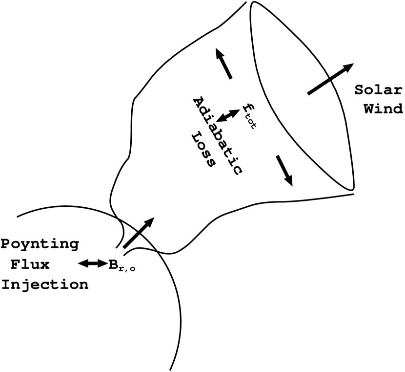
Figure 2.— Schematic picture of SW in a magnetic flux tube which is super-radially open. $B_{r,\odot}$ is proportional to Poynting flux input from the surface. $f_{\rm tot}$ determines adiabatic loss in the flux tube. Therefore, the kinetic energy of the SW in the outer region is inferred to have positive dependence on $B_{r,\odot}$ and negative dependence on $f_{\rm tot}$.

2. Formulation

I derive a simple relation which determines the SW speed near the earth from conditions on the solar surface based on a basic energy conservation relation. I consider an open magnetic flux tube measured by heliocentric distance, $r$, which is anchored at the solar surface, $r=R_{\odot}$. Under the steady-state condition, the energy equation becomes

$$\mbox{\boldmath${\nabla\cdot}$}\left[\rho\mbox{\boldmath${v}$}(\frac{v^{2}}{2}+\frac{\gamma}{\gamma-1}RT-\frac{GM_{\odot}}{r})-\frac{1}{4\pi}\mbox{\boldmath${(v\times B)\times B}$}+\mbox{\boldmath${F_{\rm c}}$}\right]+q_{\rm R}=0,$$ (1)

where $\rho$, ${v}$, $T$, ${B}$ ${F_{c}}$ and $q_{\rm R}$ are density, velocity, temperature, magnetic field strength, conductive flux and radiative cooling, respectively. $R$, $\gamma$, $G$ and $M_{\odot}$ are respectively gas constant, a ratio of specific heat, the gravitational constant and the solar mass. The term involving ${B}$ denotes Poynting flux under the ideal magnetohydrodynamical approximation. The cross section of the tube is assumed to expand in proportion to $r^{2}f(r)$, where $f(r)$ is a super-radial expansion function ($f({R_{\odot}})=1$ and $f(r_{1{\rm AU}})=f_{\rm tot}$)(Kopp & Holzer, 1976). Note that divergence of an arbitrary vector, ${A}$, becomes $\mbox{\boldmath${\nabla\cdot A}$}=\frac{1}{fr^{2}}\frac{d}{dr}(fr^{2}A_{r})$.

The Poynting flux term can be divided into two parts, $-\frac{1}{4\pi}(\mbox{\boldmath${v\times B}$})\times\mbox{\boldmath${B}$}=\frac{1}{4\pi}(-B_{r}\delta B_{\perp}\delta v_{\perp}+v_{r}\delta B_{\perp}^{2})$, where subscript $r$ denotes the component along the flux tube and $\perp$ indicates the tangential components; $\delta B_{\perp}$ and $\delta v_{\perp}$ are amplitudes of transverse fluctuations of magnetic field and velocity. The first term indicates shear of magnetic field, corresponding to Alfvén waves, and the second term denotes advection of magnetic energy.

Following FSZ, I consider the energy conservation in the flux tube between at the solar surface ($r=R_{\odot}$) and at 1AU ($r=215R_{\odot}$). At the surface, besides the gravitational potential, dynamical and magnetical energy associated with the surface convection gives an important contribution. Here I rearrange these terms concerning the inputs of energy by the convection into two parts, $-\frac{1}{4\pi}[\mbox{\boldmath${(v\times B)\times B}$}]_{r}+\rho v(\frac{v^{2}}{2}+\frac{\gamma}{\gamma-1}RT)=-\frac{1}{4\pi}B_{r}\delta B_{\perp}\delta v_{\perp}+F_{\rm H}$, namely incompressive part (Alfvén wave), $-\frac{1}{4\pi}B_{r}\delta B_{\perp}\delta v_{\perp}$, and compressive part, $F_{\rm H}$. Note that the magnetic energy term ($v_{r}\delta B_{\perp}^{2}/4\pi$) is included in $F_{\rm H}$. At 1AU the dominant term is the kinetic energy of SW (FSZ). Then, the energy conservation in the flux tube gives

$$\left[\rho vr^{2}f_{\rm tot}\frac{v^{2}}{2}\right]_{r={\rm 1AU}}=\left[r^{2}\left(-\frac{B_{r}\langle\delta B_{\perp}\delta v_{\perp}\rangle}{4\pi}+F_{\rm H}-\rho v\frac{GM_{\odot}}{r}\right)\right]_{r=R_{\odot}}-\int_{R_{\odot}}^{\rm 1AU}drr^{2}fq_{\rm R},$$ (2)

where $\langle\cdots\rangle$ denotes time-average. Thermal conduction does not appear explicitly because it only works in redistribution of the temperature structure between the two locations.

The reason of the decomposition of the energy injection terms into the two parts is that their dissipation characters are different. Generally, the dissipation of the Alfvén wave is slow since it is hardly steepen to shocks. Therefore, Alfvén waves propagate a long distance to contribute to the heating and acceleration of the SW around $\sim$ a few to $\sim 10R_{\odot}$ (SI06). On the other hand, compressive waves and turbulences denoted by $F_{\rm H}$ are more dissipative so that they only contribute to the heating in the chromosphere (Carlsson & Stein, 1992) and the low corona (Suzuki, 2002). Most of the energy of $F_{\rm H}$ which dissipates in the corona is lost by downward thermal conduction toward the chromosphere, which finally radiates away in the transition region and the upper chromosphere (Hammer, 1982). The rest ($\sim 10\%$) of the energy is transferred to enthalpy flux (Withbroe, 1988) to keep the hot corona with $T\gtrsim 10^{6}$K. The radiative cooling (last term in Equation 2) is also only efficient in the low corona or below where the density is sufficiently high. Therefore, subtraction of the radiative loss from $F_{\rm H}$ gives ‘effective’ coronal temperature, $T_{\rm C}$, namely $F_{\rm H}-\frac{1}{R_{\odot}^{2}}\int_{R_{\odot}}^{1{\rm AU}}drr^{2}fq_{\rm R}\approx\rho v\frac{\gamma}{\gamma-1}RT_{\rm C}$.

Finally, we have a conservation equation :

$$\left\{\rho vr^{2}f_{\rm tot}\frac{v^{2}}{2}\right\}_{r={\rm 1AU}}=\left\{r^{2}\left[-\frac{B_{r}\langle\delta B_{\perp}\delta v_{\perp}\rangle}{4\pi}+\rho v\left(\frac{\gamma}{\gamma-1}RT_{\rm C}-\frac{GM_{\odot}}{r}\right)\right]\right\}_{r=R_{\odot}}.$$ (3)

The second term ($\rho vr^{2}\frac{\gamma}{\gamma-1}RT_{\rm C}$) on the right hand side is evaluated at the base of the corona in the strict sense since it implicitly considers the energy balance at the transition region (see §3). However, I use the location, $r=R_{\odot}$, because the distance between the photosphere and the corona is much smaller than $R_{\odot}$. A conceptional novelty of the present formulation is that I explicitly include the Alfvén wave term which was neglected (FSZ) or parameterized in more phenomenological ways (WS91; Schwadron & McComas 2003) in previous works. Note that $-\delta B_{\perp}\delta v_{\perp}$($>0$ for outgoing Alfvén waves) is a conserved quantity of Alfvén waves which propagate in static media if they do not dissipate. Therefore, $-\langle\delta B_{\perp}\delta v_{\perp}\rangle$ is a measure of dissipation and reflection of Alfvén waves in the chromosphere and the low corona where the gas is almost static, and the results of numerical simulations (SI05; SI06) can be used for the Alfvén wave term in a straightforward manner. The physical meaning of Equation (3) is clear; the kinetic energy of the SW at 1AU is determined by positive contributions from the input Alfvén wave energy (first term) and the thermal pressure of the corona (second term) and a negative contribution due to the gravitational potential well (third term).

Rearranging Equation (3) by using the mass conservation relation, $[\rho vr^{2}f_{\rm tot}]_{r={\rm 1AU}}=[\rho vr^{2}]_{r=R_{\odot}}$, we can derive a more direct form which predicts SW speeds in the vicinity of the earth from the physical conditions on the solar surface :

$$v_{\rm 1AU}=\sqrt{2\times\left(-\frac{R_{\odot}^{2}}{4\pi(\rho vr^{2})_{\rm 1AU}}\frac{B_{r,{\odot}}}{f_{\rm tot}}\langle\delta B_{\perp}\delta v_{\perp}\rangle_{\odot}+\frac{\gamma}{\gamma-1}RT_{\rm C}-\frac{GM_{\odot}}{R_{\odot}}\right)}$$

$$= 300({\rm km/s})\sqrt{5.9\left(\frac{-\langle\delta B_{\perp}\delta v_{\perp}\rangle_{\odot}}{8.3\times 10^{5}({\rm cm\;s^{-1}G})}\right)\left(\frac{B_{r,{\odot}}{\rm(G)}}{f_{\rm tot}}\right)+3.4\left(\frac{\gamma}{1.1}\right)\left(\frac{0.1}{\gamma-1}\right)\left(\frac{T_{\rm C}}{10^{6}{\rm(K)}}\right)-4.2},$$

where I use the observed mass flux at 1AU, $(\rho v)_{\rm 1AU}=5.4\times 10^{-16}$(g cm^-2), which is almost constant even in SWs with different speeds (e.g. Aschwanden, Poland, & Rabin 2001). The velocity amplitude at the surface can be estimated from observed granulation motions at the photosphere as $\delta v_{\perp}\simeq 1$km/s (Holweger et al., 1978). The magnetic amplitude is derived from $\delta v_{\perp}$ and the photospheric density $\rho\simeq 10^{-7}$g cm^-3 as $\delta B_{\perp}=-\delta v_{\perp}\sqrt{4\pi\rho}\simeq-110$G. Then, $-\langle\delta B_{\perp}\delta v_{\perp}\rangle_{\odot}\simeq 5.5\times 10^{6}$(G cm s^-1), where a factor of 1/2 is included due to the time-average. This value is for the case in which all the Alfvén waves from the surface propagate into the SW region. In the real situation, they suffer reflection in the chromosphere. SI05 shows only $\simeq 15$% of the initial energy propagates outwardly to contributes to the heating of the coronal and SW plasma. Therefore, we adopt $-\langle\delta B_{\perp}\delta v_{\perp}\rangle_{\odot}\simeq 8.3\times 10^{5}$(G cm s^-1) as a fiducial value. As for the thermal pressure, I assume $T_{\rm C}=10^{6}$K as a typical coronal temperature. $\gamma$ should be larger than the adiabatic value ($\gamma=5/3$) because of the thermal conduction (Suess et al., 1977); I consider $\gamma=1.1$ in this paper.

3. Results and Discussions

I plot relations derived from Equation (2) in the top panel of Figure 1. The fiducial case with $\langle\delta B_{\perp}\delta v_{\perp}\rangle=8.3\times 10^{5}$(G cm s^-1) and $T_{\rm C}=10^{6}$(K) (solid line) explains the observed trend quite well. The $v_{\rm 1AU}-B_{r,{\odot}}/f_{\rm tot}$ relation reflects the Alfvén waves which accelerate the SW in expanding magnetic flux tubes. $B_{r,{\odot}}$ determines energy flux of the Alfvén waves ($\propto[B_{r}\delta B_{\perp}\delta v_{\perp}]_{\odot}$). $f_{\rm tot}$ controls ’dilution’ of the energy flux; in a flow tube with larger $f_{\rm tot}$ more energy is used to expand the tube rather than transfered to the kinetic energy of SW. Thus, the positive dependence on $B_{r,\odot}$ and the negative dependence on $f_{\rm tot}$ are naturally derived. The result does not depend on different dissipation processes of Alfvén waves because I only consider the SW speed at the sufficiently distant location ($r=1$AU) where the wave energy are mostly dissipated.

The top panel of Figure 1 also exhibits that $B_{r,\odot}/f_{\rm tot}$ is the most important parameter in determining the SW speed and that other physical conditions on the solar surface should be similar. Almost all the data are between dot-dashed and dashed lines which are the results of cases adopting slightly larger $T_{\rm C}$($=1.5\times 10^{6}$K) and smaller $\langle\delta B_{\perp}\delta v_{\perp}\rangle$ ($=5.3\times 10^{5}$G cm s^-1) than the fiducial case. Particularly, the difference of the wave amplitudes ($\delta v_{\perp}\propto\sqrt{\langle\delta B_{\perp}\delta v_{\perp}\rangle}$) between the solid and dashed lines are only 20%. This indicates that the amplitudes of Alfvén waves at the surface should be very similar in different coronal holes. The observed data are from not only polar coronal holes but mid-latitude and equatorial coronal holes, some of which are located near active regions. Therefore, one can infer that the amplitudes could vary a lot since the circumstances are quite different. However, the observation seems to favor the constancy of the Alfvénic fluctuations at the footpoints. Although it is very difficult to observe Alfvénic motions of field lines on the solar surface at present (Ulrich, 1996), this can be observationally studied in the very near future by Solar-B satellite which can stably observe fine-scale motions of surface magnetic fields.

Let me compare the present analysis with a model calculation for the $v_{\rm 1AU}-1/f_{\rm tot}$ correlation by WS91 (see also Wang (1993)). Although it is not simple to compare both since the assumptions adopted in WS91 are different from mine (for example, WS91 fixed the coronal base density, while I adopt the constant mass flux at 1AU), I can derive a relation of $v_{\rm 1AU}-1/f_{\rm tot}$ from Equation (2) by using similar constraints to those considered in WS91. They adopted a constant field strength at 1AU, $B_{r,{\rm 1AU}}=3\times 10^{-5}$G, and assumed a constant energy flux ($=1.5\times 10^{5}$erg cm^-2s^-1) at the coronal base. In the middle panel of Figure 1, I present the result with fixed $B_{r,\odot}/f_{\rm tot}=1.4$, corresponding to $B_{r,\odot}=3\times 10^{-5}$G, and energy flux of Alfvén waves, $B_{r,\odot}\langle\delta B_{\perp}\delta v_{\perp}\rangle/4\pi=4\times 10^{5}$erg cm^-2s^-1 (i.e. $\langle\delta B_{\perp}\delta v_{\perp}\rangle\propto f_{\rm tot}^{-1}$) in Equation (2) by the dotted line. Note that I need the larger energy flux because the inner boundary is not the coronal base but the photosphere. The figure shows that the dotted line follows the average trend of the data and the result of WS91 is reasonable. However, I would like to address that some data are located away from the main $v_{\rm 1AU}-1/f_{\rm tot}$ trend and they can be explained in a unified manner by taking into account $B_{r,\odot}$.

The relation of Equation (2) seemingly contradicts to the reported anti-correlation of the coronal temperature and the SW speed (Geiss et al., 1995). This is because my treatment of the thermal processes near the surface is too much simplified; the complicated energy balance from the chromosphere to the low corona is represented only by the ‘effective’ enthalpy, $\frac{\gamma}{\gamma-1}RT_{\rm C}$. The formulation for the temperature-velocity relation by Schwadron & McComas (2003) is complementary to the present formulation. In Schwadron & McComas (2003) the detailed energy balance at the transition region is taken into account, while they assumed a constant input of the Alfvén wave energy flux which I investigate more in detail.

In this letter, in order to focus on the SW speed, I simply apply the observed (almost) constant mass flux at 1AU when deriving the relation for the SW speed. For self-consistent treatments, however, it is important to study how to determine the mass flux of the SW not only by numerical simulations (e.g. SI06) but by simple models.

I think that Equation (2) is applicable to SWs during both sunspot minimum and maximum phases because it is derived based only on the simple energetics. At present, however, the observed data (Kojima et al.2005) which I use for the comparison are only during the sunspot minimum phase (1995-1996). In order to study the generality of the derived relation, comparisons with SW data during different phases (Fujiki et al.2006) are important. One should be careful that $f_{\rm tot}$ which should be used for the prediction is the actual super-radial expansion factor from $R_{\odot}$ to 1AU, while in most cases, including Kojima et al. (2005), $f_{\rm tot}$ is observationally estimated from the comparison between at $R_{\odot}$ and at the source surface ($2.5R_{\odot}$) based on the potential field-source surface method. Errors due to this method could be non-negligible if the potential approximation becomes worse and/or if one separately treats flux tubes in a coronal hole (WS90). (In this sense, Kojima et al.2005 as well as I use $B_{r,\odot}/f_{\rm tot}$ instead of field strength at the source surface.) Thus, the precise determination of coronal magnetic fields (e.g. Linker et al.1999) is important for reliable forecasts of SW speeds from the relation of Equation (2).

The author thank the solar wind group in Nagoya-STEL (Kojima, M., Tokumaru, M., Fujiki, K.) for fruitful discussions and providing observational data. The author also thank the referee for constructive comments. This work is supported by the JSPS Research Fellowship for Young Scientists, grant 4607.

References

- Arge & Pizzo (2000) Arge, C. N. & Pizzo, V. J. 2000, J. Geophys. Res., 105, 10465
- Aschwanden, Poland, & Rabin (2001) Aschwanden, M. J., Poland, A. I., & Rabin, D. M. 2001, ARA&A, 39, 175
- Belcher (1971) Belcher, J. W. 1971, ApJ, 168, 509
- Carlsson & Stein (1992) Carlsson, M. & Stein, R., F. 1992, ApJ, 397, L59
- Cranmer (2005) Cranmer, S. R. 2005, Proc. of Solar Wind 11/SOHO16, 159
- Fisk, Schwadron, & Zurbuchen (1999) Fisk, L. A., Schwadron, N. A., & Zurbuchen, T. H. 1999 J. Geophys. Res., 104, A4, 19765 (FSZ)
- Fujiki et al. (2006) Fujiki, K. et al. 2006, in preparation
- Geiss et al. (1995) Geiss, J. et al. 1995, Science, 268, 1033
- Hakamada & Kojima (1999) Hakamada, K. & Kojima, M. 1999, Sol. Phys., 187, 115
- Hammer (1982) Hammer, R. 1982, ApJ, 259, 767
- Holweger et al. (1978) Holweger, H., Gehlsen, M., & Ruland, F. 1978, A&A, 70, 537
- Jacques (1977) Jacques, S. A. 1977, ApJ, 215, 942
- Kojima et al. (2005) Kojima, M., K. Fujiki, M. Hirano, M. Tokumaru, T. Ohmi, and K. Hakamada, 2005, ”The Sun and the heliosphere as an Integrated System”, G. Poletto and S. T. Suess, Eds. Kluwer Academic Publishers, 147
- Kopp & Holzer (1976) Kopp, R. A. & Holzer, T. E. 1976, Sol. Phys., 49, 43
- Linker et al. (1999) Linker et al. 1999, J. Geophys. Res., 104, 9809
- McIntosh & Leamon (2005) McIntosh, S. W. & Leamon, R. J. 2005, ApJ, 624, L117
- Ofman (2004) Ofman, L. 2004, J. Geophys. Res., 109, A07102
- Phillips et al. (1995) Phillips, J. L. et al. 1995, Geophys. Res. Lett., 22, 3301
- Sakurai (1982) Sakurai, T. 1982, Sol. Phys., 76, 301
- Schwadron & McComas (2003) Schwadron, N. A. & McComas, D. J. 2003, ApJ, 599, 1395
- Suess et al. (1977) Suess, S. T., Richter, A. K., Winge, C. R., & Nerney, S. F. 1977, ApJ, 217, 296
- Suess et al. (1984) Suess, S. T., Wolcox, J. M., Hoeksema, J. T., Henning, H., & Dryer, M. 1984, J. Geophys. Res., 89, 3957
- Suzuki (2002) Suzuki, T. K. 2002, ApJ, 578, 598
- Suzuki & Inutsuka (2005) Suzuki, T. K. & Inutsuka, S. 2005, ApJ, 632, L49 (SI05)
- Suzuki & Inutsuka (2006) Suzuki, T. K. & Inutsuka, S. 2006, JGR submitted (astro-ph/0511006) (SI06)
- Ulrich (1996) Ulrich, R. K. 1996, ApJ, 465, 436
- Wang & Sheeley (1990) Wang, Y.-M. & Sheeley, Jr, N. R. 1990, ApJ, 355, 726 (WS90)
- Wang & Sheeley (1991) Wang, Y.-M. & Sheeley, Jr, N. R. 1991, ApJ, 372, L45 (WS91)
- Wang (1993) Wang, Y.-M. 1993, ApJ, 410, L123
- Withbroe (1988) Withbroe, G. L. 1988, ApJ, 325, 442
- Wu & Lepping (2002) Wu, C. C. & Lepping, R. P. 2002, J. Geophys. Res., 107, A11, SSH3-1 (2002)