Evolving Newton’s Constant, Extended Gravity Theories and SnIa Data Analysis

Abstract

If Newton’s constant $G$ evolves on cosmological timescales as predicted by extended gravity theories then Type Ia supernovae (SnIa) can not be treated as standard candles. The magnitude-redshift datasets however can still be useful. They can be used to simultaneously fit for both $H(z)$ and $G(z)$ (so that local $G(z)$ constraints are also satisfied) in the context of appropriate parameterizations. Here we demonstrate how can this analysis be done by applying it to the Gold SnIa dataset. We compare the derived effective equation of state parameter $w(z)$ at best fit with the corresponding result obtained by neglecting the evolution $G(z)$. We show that even though the results clearly differ from each other, in both cases the best fit $w(z)$ crosses the phantom divide $w=-1$. We then attempt to reconstruct a scalar tensor theory that predicts the derived best fit forms of $H(z)$ and $G(z)$. Since the best fit $G(z)$ fixes the scalar tensor potential evolution $F(z)$, there is no ambiguity in the reconstruction and the potential $U(z)$ can be derived uniquely. The particular reconstructed scalar tensor theory however, involves a change of sign of the kinetic term $\Phi^{\prime}(z)^{2}$ as in the minimally coupled case.

I Introduction

A diverse set of cosmological observations including the abundance of galaxy clusters lss , the baryon fraction in galaxy clusters bfrac , statistics of large scale redshift surveys lsstat , and the angular power spectrum of the Cosmic Microwave Background (CMB) cmb indicate that the universe is flat and that there is a low value of the matter density parameter $0.16<\Omega_{0m}<0.35$. Thus, in the context of standard general relativistic cosmology there is a gap between $\Omega_{0m}$ and $\Omega_{tot}=1$ required for flatness. This gap is usually assumed to be filled by an unknown form of energy called dark energydark energy . In addition, the magnitude-redshift relation for type Ia supernovae (SnIa) snobs ; Riess:2004nr ; snls , which can probe the recent expansion history of the universe indicates that the universe has entered a phase of accelerating expansion (the scale factor obeys ${\ddot{a}}>0$). This can be reconciled with the other cosmological data by assuming that the dark energy has negative pressure and therefore has repulsive gravitational properties (see Perivolaropoulos:2006ce for a recent review).

The dark energy component is usually described by an equation of state parameter $w\equiv{p\over\rho}$ (the ratio of the homogeneous dark energy pressure $p$ over the energy density $\rho$). For cosmic acceleration, a value of $w<-{1\over 3}$ is required as indicated by the Friedmann equation

$${{\ddot{a}}\over a}=-{{4\pi G}\over 3}(\rho+3p)$$ (1)

The simplest viable example of dark energy is the cosmological constant ($w=-1$). This example however even though consistent with present data lacks physical motivation. Questions like ‘What is the origin of the cosmological constant?’ or ‘Why is the cosmological constant $10^{120}$ times smaller than its natural scale $M_{pl}$ so that it starts dominating at recent cosmological times (coincidence problem)?’ remain unanswered. Attempts to replace the cosmological constant by a dynamical scalar field (quintessencequintess ) which may also couple to dark matter coupdm , have created a new problem regarding the initial conditions of quintessence which even though can be resolved in particular cases (tracker quintessence), can not answer the above questions in a satisfactory way.

An alternative approach towards understanding the nature of dark energy is to attribute it to extensions of general relativitymodgrav on cosmological scales. Such extensions can be expressed for example through scalar-tensor theoriesEsposito-Farese:2000ij . In these theories the Einstein Lagrangian of general relativity is replaced by a generalized Lagrangian of the form

$${\cal L}=\frac{F(\Phi)}{2}~{}R-\frac{Z(\Phi)}{2}~{}g^{\mu\nu}\partial_{\mu}\Phi\partial_{\nu}\Phi-U(\Phi)+{\cal L}_{m}[\psi_{m};g_{\mu\nu}]\$$ (2)

where we have set $8\pi G=1$ ($F_{0}=1$) and ${\cal L}_{m}$ represents the matter fields and does not depend on $\Phi$ so that the weak equivalence principle is satisfied. A common choice in the Jordan frame is to set $Z\rightarrow 1$ by rescaling the field $\Phi$ Esposito-Farese:2000ij .

The evolution of Newton’s constant predicted in the context of extended gravity theories requires special care when comparing the predictions of these theories with observationsAcquaviva:2004ti . This evolution induces special effects to the physics of SnIa Amendola:1999vu ; Garcia-Berro:1999bq ; Gaztanaga:2001fh ; Riazuelo:2001mg . The observed magnitude redshift relation of SnIa can be translated to luminosity distance-redshift relation (which leads to the expansion history $H(z)$) only under the assumption that SnIa behave as standard candles. This assumption is justified in view of the fact that the observational light curves of closeby SnIa are well understood and their individual intrinsic differences can be accounted for. Nevertheless, since the accelerated expansion of the universe is based on the fact that the peak luminosities of distant supernovae appear to be $\sim 0.20$ magnitude fainter than predicted for an empty universe and $\sim 0.25$ magnitude fainter than a decelerating universe with $\Omega_{0m}=0.3$, it is clear that even minor unaccounted evolutionary effects can drastically change our current view for accelerating universe. The possible consequences of evolutionary effects in SnIa due to changes in the zero age mass and metallicity of the progenitor star have been previously explored Dominguez:1998jt who found that changes in the underlying population cause a change in the maximum brightness by about $0.1-0.2$ magnitudes.

The corresponding evolutionary effects due to the evolution of $G$ in scalar tensor theories have also been studied Riazuelo:2001mg ; Garcia-Berro:1999bq . The peak luminosity of SnIa is proportional Gaztanaga:2001fh to the mass of nickel synthesized which is a fixed fraction of the Chandrasekhar mass $M_{Ch}$ varying as $M_{Ch}\sim G^{-3/2}$. Therefore the SnIa peak luminosity varies like $L\sim G^{-3/2}$ and the corresponding SnIa absolute magnitude evolves like

$$M-M_{0}=\frac{15}{4}log\frac{G}{G_{0}}$$ (3)

where the subscript $0$ denotes the local values of $M$ and $G$. Thus, the magnitude-redshift relation of SnIa in the context of extended gravity theories is connected with the luminosity distance $d_{L}(z)$ as

$$m_{th}(z)=M_{0}+5logd_{L}(z)+\frac{15}{4}log\frac{G(z)}{G_{0}}$$ (4)

In the limit of constant $G$ this reduces to the familiar result. On the other hand, in scalar tensor theoriesEsposito-Farese:2000ij we have

$$\frac{G(z)}{G_{0}}=\frac{1}{F}\frac{2F+4(dF/d\Phi)^{2}}{2F+3(dF/d\Phi)^{2}}\simeq\frac{1}{F}$$ (5)

and solar system experiments Will:2005va ; will-bounds indicate that $\frac{dF(\Phi)}{d\Phi}\sim\frac{dF(z)}{dz}\simeq 0$. Assuming flatness, the expansion history $H(z)$ is obtained from

$$d_{L}(z)=(1+z)\int_{0}^{z}dz^{\prime}\sqrt{\frac{G_{0}}{G(z^{\prime})}}\frac{1}{H(z^{\prime})}$$ (6)

Therefore, by fitting $m_{th}$ of (4) to the observed Gold SnIa Riess:2004nr dataset expressed as $m_{obs}(z_{i})$ and using (5) and (6) we may obtain the best fit forms of both $H(z)$ and $G(z)$ assuming appropriate parameterizations. It should be pointed out that even though the modified magnitude-redshift relation (4) has been known for some time Garcia-Berro:1999bq , it has not been properly utilized in studies attempting to constrain extended theories of gravity with SnIa data (see eg Caresia:2003ze ). This task is undertaken in what follows.

The structure of this paper is the following: In the next section we use simple polynomial parameterizations of $G(z)$ and $H(z)$ to fit these functions to the Gold dataset using equations (4) and (6). In section III we use the best fits of $G(z)$ and $H(z)$ to construct the best fit scalar tensor theory ie the potential $U(z)$ and the form of $\Phi^{\prime}(z)^{2}$. Finally in section IV we conclude, summarize and discuss possible implications of our results.

II Fitting $G(z)$ and $H(z)$ to the Gold dataset

The recent expansion history of the universe is best probed by using a diverse set of cosmological data including SnIa standard candles, CMB spectrum, large scale structure power spectrum, weak lensing surveys etc. Given the present quality of cosmological data, among the above cosmological observations the most sensitive and high quality probe of the recent expansion history $H(z)$ is the magnitude-redshift relation of SnIa. This probe will be used in the present study.

There have been two approaches in derivingphant-obs2 the functions $d_{L}(z)$, $H(z)$ and $w(z)$ from the discrete set of magnitude-redshift data and their errorbars. According to the first approachShafieloo:2005nd , a smoothing window function is used to derive a continuous function $m(z)$ (or equivalently $d_{L}(z)$) assuming no evolution of $G$ in equation (4)) and then $H(z)$ and $w(z)$ are obtained using the well known relations Sahni:2004ai

$$H(z)=c[{d\over{dz}}({{d_{L}(z)}\over{1+z}})]^{-1}$$ (7)

and

$$w(z)={{p_{DE}(z)}\over{\rho_{DE}(z)}}={{{2\over 3}(1+z){{d\ln H}\over{dz}}-1}\over{1-({{H_{0}}\over H})^{2}\Omega_{0m}(1+z)^{3}}}$$ (8)

This approach works well in the context of general relativity where $G(z)=G_{0}$ but it can not be used in the context of scalar-tensor theories (unless supplemented by additional cosmological observations) because equation (4) alone can not be used to derive both $d_{L}(z)$ and $G(z)$ from the single smoothed function $m(z)$. In fact, even if a smoothed form of $d_{L}(z)$ was obtained it would be hard to disentangle $H(z)$ from $G(z)$ in equation (6).

The second approachalam1 ; nesper ; Lazkoz:2005sp ; Weller:2001gf is based on assigning particular parameterizations (which are consistent with other observations) to the function $H(z)$ (and to $G(z)$ if applicable) involving two to three parameters and fitting these parameters to the magnitude-redshift data. The goodness of fit corresponding to any set of parameters $a_{1},...,a_{n}$ is determined by the probability distribution of $a_{1},...,a_{n}$ i.e.

$$P({\bar{M}},a_{1},...,a_{n})={\cal N}e^{-\chi^{2}({\bar{M}},a_{1},...,a_{n})/2}$$ (9)

where

$$\chi^{2}({\bar{M}},a_{1},...,a_{n})=\sum_{i=1}^{157}\frac{(m^{obs}(z_{i})-m^{th}(z_{i};{\bar{M}},a_{1},...,a_{n}))^{2}}{\sigma_{m^{obs}(z_{i})}^{2}}$$ (10)

and ${\cal N}$ is a normalization factor. If prior information is known on some of the parameters $a_{1},...,a_{n}$ then we can either fix the known parameters using the prior information or ‘marginalize’, i.e. average the probability distribution (9) around the known value of the parameters with an appropriate ‘prior’ probability distribution.

The parameters ${\bar{a}}_{1},...,{\bar{a}}_{n}$ that minimize the $\chi^{2}$ expression (10) are the most probable parameter values (the ‘best fit’) and the corresponding $\chi^{2}({\bar{a}}_{1},...,{\bar{a}}_{n})\equiv\chi_{min}^{2}$ gives an indication of the quality of fit for the given parametrization: the smaller $\chi_{min}^{2}$ the better the parametrization. The minimization with respect to the parameter $\bar{M}$ can be made trivially by expanding the $\chi^{2}$ of equation (10) with respect to $\bar{M}$ asLazkoz:2005sp

$$\chi^{2}(a_{1},..,a_{n})=A-2{\bar{M}}B+{\bar{M}}^{2}C$$ (11)

where

$$A(a_{1},..,a_{n}) = \sum_{i=1}^{157}\frac{(m^{obs}(z_{i})-m^{th}(z_{i};{\bar{M}}=0,a_{1},..,a_{n}))^{2}}{\sigma_{m^{obs}(z_{i})}^{2}}$$

$$B(a_{1},..,a_{n}) = \sum_{i=1}^{157}\frac{(m^{obs}(z_{i})-m^{th}(z_{i};{\bar{M}}=0,a_{1},..,a_{n}))}{\sigma_{m^{obs}(z_{i})}^{2}}$$

$$C = \sum_{i=1}^{157}\frac{1}{\sigma_{m^{obs}(z_{i})}^{2}}$$ (12)

Equation (11) has a minimum for ${\bar{M}}={B}/{C}$ at

$$\chi^{\prime 2}(a_{1},...,a_{n})=A(a_{1},...,a_{n})-\frac{B(a_{1},...,a_{n})^{2}}{C}$$ (13)

Thus instead of minimizing $\chi^{2}({\bar{M}},a_{1},...,a_{n})$ we can minimize $\chi^{\prime 2}(a_{1},...,a_{n})$ which is independent of ${\bar{M}}$. Obviously $\chi_{min}^{2}=\chi_{min}^{{}^{\prime}2}$.

The errors are evaluated using the covariance matrix of the fitted parameters press92 and the error on any cosmological quantity, e.g. the equation of state $w(z;p_{i})$, is given by:

$$\sigma_{w}^{2}=\sum_{i=1}^{n}(\frac{\partial w}{\partial p_{i}})C_{ii}+2\sum_{i=1}^{n}\sum_{j=i+1}^{n}(\frac{\partial w}{\partial p_{i}})(\frac{\partial w}{\partial p_{j}})C_{ij}$$ (14)

where $p_{i}$ are the cosmological parameters and $C_{ij}$ the covariance matrix Alam:2004ip .

We considered simple polynomial parameterizations for the functions $H(z)$ and $G(z)$ of the form

$$H^{2}(z) = H_{0}^{2}\{\Omega_{0m}(1+z)^{3}+a_{1}(1+z)+a_{2}(1+z)^{2}+$$ (15)

$$(1-\Omega_{0m}-a_{1}-a_{2})\}$$

$$G(z) = G_{0}\;(1+a\;z^{2})$$ (16)

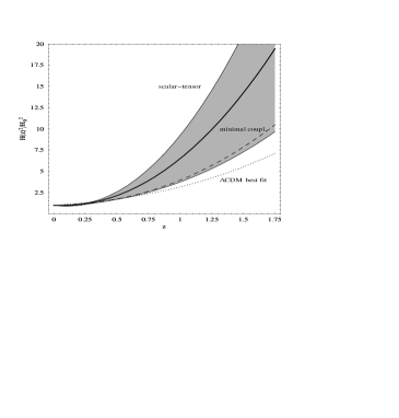
Figure 1: The best fit form of $H(z)$ in the scalar tensor (continuous line), minimally coupled (dashed line) and $\Lambda$CDM (dotted) cases. The shaded region corresponds to the $1\sigma$ region of the scalar-tensor best fit.

where the linear term in $G(z)$ has been ignored due to experimental constraints on scalar tensor theories will-bounds . Using the parameterizations (15) and (16) we have minimized the $\chi^{\prime 2}$ of (13) using the 157 datapoints of the Gold dataset and equations (4), (6). We used a prior of $\Omega_{0m}=0.23$ wmap3 and we verified that our results are relatively insensitive to the prior of $\Omega_{0m}$ used in the range $0.18<\Omega_{0m}<0.32$. The minimum was obtained at $\chi^{2}=173.045$ for $a_{1}=-12.35\pm 8.55$, $a_{2}=5.41\pm 3.82$ and $a=0.05\pm 0.04$. We compared our results with the corresponding minimally coupled case obtained by fixing $a=0$ before minimization (setting $G(z)=G_{0}$ at all times). The corresponding minimum was obtained at $\chi^{2}=174.168$ for $a_{1}=-4.54\pm 2.52$, $a_{2}=1.96\pm 1.09$.

The best fit functions for $H(z)$, $w(z)$ and $F(z)=\frac{1}{G(z)}$ for both the scalar-tensor and minimally coupled cases are shown in Figs. 1, 2 and 3 respectively along with the $1\sigma$ (shaded) region of the scalar-tensor best fit.

An interesting feature of Fig. 3 is the relatively large (about 15$\%$) cosmological variation of Newton’s constant. In Umezu:2005ee it is shown that CMB and SDSS constraints allow Newton’s constant to vary by a factor of 2 on cosmological scales. The variation implied by our analysis is about $15\%$ and is well within the cosmological constraints.

Also, it is clear that the best fit equation of state parameter $w(z)$ crosses the phantom divide in both the scalar-tensor and the minimally coupled case at about $z\simeq 0.2$. This type of crossing which seems to be favored by the Gold SnIa dataset crossgold ; alam1 ; nesper ; Lazkoz:2005sp (but not nocrossnls ; nocrossnls1 by the more recent first year SNLS dataset snls ) has been the subject of extensive studies in the literaturecrosstud as its reproduction is highly non-trivial in the context of most theoretical modelsVikman:2004dc .

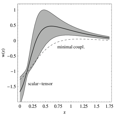
Figure 2: The best fit form of $w(z)$ in the scalar tensor (continuous line) and minimally coupled (dashed line) cases.

In the scalar-tensor case $w(z)$ does not have the usual meaning of the dark energy equation of state but it is merely defined in terms of $H(z)$ as in equation (8). In particular we use $w(z)$ simply as an alternative way of plotting $H(z)$. Such a way is useful for comparing with other analyses Sahni:2004ai ; alam1 based on dark energy. Those analyses also derive their best fit $w(z)$ from their best fit $H(z)$ but they simply interpret the derived best fit $w(z)$ as an equation of state parameter. Therefore even though the interpretation is different, the comparison is meaningful since the actual quantity that is compared is $H(z)$. The best fit functions $H(z)$ and $F(z)$ will be used in the next section to complete the construction of the best fit scalar tensor theory from the Gold dataset.

III Reconstructing the Scalar-Tensor Lagrangian

The derived best fit functions $F(z)$ and $H(z)$ may now be used as input Perivolaropoulos:2005yv ; Tsujikawa:2005ju in the field equations obtained from the Lagrangian (2) in a cosmological setup to obtain the potential $U(z)$ and the field kinetic term $\Phi^{\prime}(z)^{2}$.

Assuming a homogeneous $\Phi$ and varying the action corresponding to (2) in background of a flat FRW metric

$$ds^{2}=-dt^{2}+a^{2}(t)(dr^{2}+r^{2}\left(d\theta^{2}+\sin^{2}\theta~{}d\phi^{2}\right))$$ (17)

we find the coupled system of equationsEsposito-Farese:2000ij

$$3F\cdot H^{2} = \rho+{1\over 2}\dot{\Phi}^{2}-3H\cdot\dot{F}+U$$ (18)

$$-2F\cdot\dot{H} = (\rho+p)+\dot{\Phi}^{2}+\ddot{F}-H\cdot\dot{F}$$ (19)

where we have assumed the presence of a perfect fluid $(\rho,p)$. Eliminating $\dot{\Phi}^{2}$ from (19), setting

$$q(z)\equiv H(z)^{2}/H_{0}^{2}$$ (20)

and rescaling $U\rightarrow U\cdot H_{0}^{2}$ while expressing in terms of redshift $z$ we obtain

$$F^{\prime\prime} + \left[\frac{q^{\prime}}{2q}-\frac{4}{1+z}\right]~{}F^{\prime}+\left[\frac{6}{(1+z)^{2}}-\frac{2}{(1+z)}\frac{q^{\prime}}{2q}\right]~{}F=\frac{2U}{(1+z)^{2}q^{2}}+3\frac{1+z}{q^{2}}\Omega_{0m}\$$ (21)

$$\Phi^{\prime 2} = -{6F^{\prime}\over 1+z}+{6F\over(1+z)^{2}}-{{2U}\over(1+z)^{2}q^{2}}-6\frac{1+z}{q^{2}}\Omega_{0m}$$ (22)

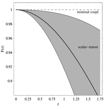
Figure 3: The best fit form of $F(z)=1/G(z)$ in the scalar tensor (continuous line) and minimally coupled (dashed line) cases. Due to experimental constraints $F(z)$ displays an extremum at the present time. Consistency with the SnIa data requires that this extremum be a maximum for $F(z)$ (minimum for $G(z)$).

where the prime ^′ denotes differentiation with respect to redshift $(\frac{d}{dz})$ and we have assigned properties of matter ($p=0,\;\Omega_{0m}=\frac{3\rho_{0m}}{H_{0}^{2}}$) to the perfect fluid.

Given the best fit form of $F(z)$ and $H(z)$ obtained in the previous section from observations, equations (21) and (22) may be used to reconstruct the $U(z)$ and $\Phi^{\prime}(z)^{2}$ which predict the best fit forms of $H(z)$ ($q(z)$) and $F(z)$ for both the minimally coupled and the scalar-tensor cases. The resulting forms of $U(z)$ and $\Phi^{\prime}(z)^{2}$ are shown in Figs 4 and 5 respectively.

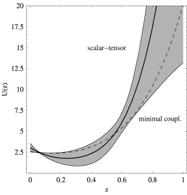
Figure 4: The redshift evolution of the potential for the best fit forms of $H(z)$ and $F(z)$ for the scalar-tensor (continuous line) and minimally coupled (dashed line) cases.

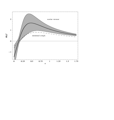
Figure 5: The redshift evolution of the kinetic term $\Phi^{\prime}(z)^{2}$ for the best fit forms of $H(z)$ and $F(z)$ for the scalar-tensor (continuous line) and minimally coupled (dashed line) cases. The change of sign at a redshift $z\simeq 0.2$ creates problems for both classes of theories.

An interesting feature of Fig. 5 is the change of sign of $\Phi^{\prime 2}(z)$ that is predicted for both classes of theories (at best fit) at a redshift $z\simeq 0.2$ (the same redshift where the phantom divide barrier is crossed). This creates a serious challenge for both classes of theories. This problem was well known for minimally coupled theories but it was believed that scalar-tensor theories which have the potential to cross the phantom divide in a self consistent way Boisseau:2000pr ; Perivolaropoulos:2005yv could bypass this problem. Our result however indicates that if the SnIa evolution is taken into account then scalar-tensor theories are faced with a similar problem as minimally coupled modelsVikman:2004dc in the context of the Gold SnIa dataset.

As discussed in Ref. nocrossnls , the Gold dataset mildly favours dynamical dark energy compared to $\Lambda$CDM while the SNLS dataset favours $\Lambda$CDM even in the context of dynamical parameterizations. Thus we anticipate that in the case of the SNLS dataset both of the best fit curves of Fig 2 (for the scalar-tensor and minimally coupled cases) would tend to be closer to the w=-1 line. In fact, the minimally coupled case with the SNLS dataset has been discussed in Ref. nocrossnls in the context of the polynomial parameterizations of eq. (2.9).

IV Conclusion

We have constructed a method to utilize the magnitude redshift SnIa data in the context of extended gravity theories. Assuming simple redshift parameterizations for $H(z)$ and $G(z)$ we have found their best fit forms and the corresponding error regions. The best fit form of $G(z)$ indicates a slowly decreasing Newton’s constant (increasing $F(z)=\frac{1}{G(z)}$) at recent cosmological times. The corresponding best fit form of $w(z)$ (defined through eq. (8)) was found to cross the phantom divide $w=-1$ for both a constant and a redshift dependent $G$. However, in the later case the best fit $w(z)$ was found to vary more rapidly with redshift.

The simultaneous knowledge of both $F(z)$ and $H(z)$ allows the unambiguous reconstruction of a scalar tensor theory by solving the generalized Friedman equations. The particular reconstructed scalar tensor theory using the Gold SnIa dataset and the specific parameterizations, turned out to suffer from a similar problem as the corresponding minimally coupled theory (the kinetic term changes sign at a recent redshift). We have also considered more complicated parameterizations for $G(z)$ and $H(z)$ which however had only a minor effect on our results and did not seem to alleviate the above mentioned problem.

Thus, if the best fit forms of $H(z)$ and $G(z)$ are verified by future SnIa datasets, this would indicate that neither minimally coupled nor extended quintessence are realized in Nature. In that case the SnIa data could possibly be consistent with either alternative extensions of general relativity (eg brane worldsmodgrav ) or by a combination of phantom + quintessence scalars (quintom modelsGuo:2004fq ) (see also Stefancic:2005cs ; Caldwell:2005ai ; Hu:2004kh for alternative approaches). An interesting extension of the present work would be to use the best fit forms of $H(z)$ and $G(z)$ obtained from SnIa and other cosmological data, in an attempt to reconstruct consistently alternative extended gravity theories.

The Mathematica file with the numerical analysis of the paper can be found at http://leandros.physics.uoi.gr/snevol.html .

Acknowledgements: This research was funded by the program PYTHAGORAS-1 of the Operational Program for Education and Initial Vocational Training of the Hellenic Ministry of Education under the Community Support Framework and the European Social Fund. SN acknowledges support from the Greek State Scholarships Foundation (I.K.Y.).

References

- (1) N.A.Bahcall et al, Science284,1481 (1999); Percival, W.J., et al., Mon. Not. Roy. Ast. Soc. 327, 1297 (2001); M. Tegmark et al. [SDSS Collaboration], Phys. Rev. D 69, 103501 (2004) [arXiv:astro-ph/0310723].
- (2) V. Hradecky, C. Jones, R. H. Donnelly, S. G. Djorgovski, R. R. Gal and S. C. Odewahn, arXiv:astro-ph/0006397; S. W. Allen, R. W. Schmidt and A. C. Fabian, Mon. Not. Roy. Astron. Soc. 334, L11 (2002) [arXiv:astro-ph/0205007].
- (3) W. J. Percival et al. [The 2dFGRS Collaboration], Mon. Not. Roy. Astron. Soc. 327, 1297 (2001) [arXiv:astro-ph/0105252]; L. Verde et al., Mon. Not. Roy. Astron. Soc. 335, 432 (2002) [arXiv:astro-ph/0112161].
- (4) D. N. Spergel et al. [WMAP Collaboration], Astrophys. J. Suppl. 148, 175 (2003) [arXiv:astro-ph/0302209].
- (5) M. S. Turner and M. White, Phys. Rev. D56, R4439 (1997); T. Padmanabhan,Curr. Sci. 88, 1057 (2005)[arXiv:astro-ph/0411044]. P. H. Frampton, arXiv:astro-ph/0409166; V. Sahni, arXiv:astro-ph/0403324.
- (6) Riess A et al., 1998 Astron. J. 116 1009; Perlmutter S J et al., 1999 Astroph. J. 517 565; Bull.Am.Astron.Soc29,1351(1997); Tonry, J L et al., 2003 Astroph. J. 594 1; Barris, B et al., 2004 Astroph. J. 602 571; Knop R et al., 2003 Astroph. J. 598 102;
- (7) A. G. Riess et al. [Supernova Search Team Collaboration], Astrophys. J. 607, 665 (2004) [arXiv:astro-ph/0402512].
- (8) P. Astier et al.,Astron. Astrophys. 447 31-48 (2006), arXiv:astro-ph/0510447.
- (9) L. Perivolaropoulos, arXiv:astro-ph/0601014.
- (10) B.Ratra and P.J.E.Peebles, Phys.Rev. D37,3406(1988); astro-ph/0207347; C.Wetterich, Nucl. Phys. B302,668(1988); P.G.Ferreira and M.Joyce, Phys. Rev. D.58,023503(1998); P.Brax and J.Martin, Phys. Rev. D.61,103502(2000); D.Wands, E.J.Copeland and A.R.Liddle, Phys. Rev. D.57,4686 (1998); A.R. Liddle and R.J. Scherrer, Phys. Rev. D 59, 023509 (1998); R.R. Caldwell, R. Dave and P. Steinhardt, Phys. Rev. Lett 80, 1582 (1998); I. Zlatev, L. Wang and P. Steinhardt, Phys. Rev. Lett. 82, 896 (1999); S. Dodelson, M. Kaplinghat and E. Stewart, Phys. Rev. Lett. 85, 5276(2000); V.B.Johri, Phys. Rev. D.63,103504(2001); V.Sahni and L.Wang, Phys. Rev. D.62,103517(2000); M. Axenides and K. Dimopoulos, JCAP 0407, 010 (2004)[arXiv:hep-ph/0401238].
- (11) B. Gumjudpai, T. Naskar, M. Sami and S. Tsujikawa, JCAP 0506, 007 (2005) [arXiv:hep-th/0502191]; S. Tsujikawa, arXiv:hep-th/0601178; P. P. Avelino, L. M. G. Beca, J. P. M. de Carvalho, C. J. A. Martins and E. J. Copeland, Phys. Rev. D 69, 041301 (2004)[arXiv:astro-ph/0306493].
- (12) V. Sahni and Y. Shtanov, IJMP D11, 1515 (2002); JCAP 0311, 014 (2003); S. Nojiri, S. D. Odintsov and M. Sasaki, Phys. Rev. D 71, 123509 (2005) [arXiv:hep-th/0504052]; M. Sami, A. Toporensky, P. V. Tretjakov and S. Tsujikawa, Phys. Lett. B 619, 193 (2005) [arXiv:hep-th/0504154]; L. Perivolaropoulos and C. Sourdis, Phys. Rev. D 66, 084018 (2002) [arXiv:hep-ph/0204155]; C. Deffayet, G. Dvali and G. Gabadadze, Phys. Rev. D65, 044023 (2002); J. S. Alcaniz, Phys. Rev. D 65, 123514 (2002) astro-ph/0202492; E. V. Linder, Phys. Rev. Lett. 90, 091301 (2003) [arXiv:astro-ph/0208512]; L. Perivolaropoulos, Phys. Rev. D 67, 123516 (2003) [arXiv:hep-ph/0301237]; D.F.Torres, Phys. Rev. D66,043522(2002); S. Nojiri and S. D. Odintsov, Proc. Sci. WC2004, 024 (2004) [arXiv:hep-th/0412030]; E. Elizalde, S. Nojiri and S. D. Odintsov, Phys. Rev. D 70, 043539 (2004) [arXiv:hep-th/0405034]; S. Nojiri and S. D. Odintsov,arXiv:hep-th/0601213; P. P. Avelino and C. J. A. Martins, Astrophys. J. 565, 661 (2002) [arXiv:astro-ph/0106274];B. M. N. Carter and I. P. Neupane, arXiv:hep-th/0512262;I. P. Neupane, Class. Quant. Grav. 21, 4383 (2004) [arXiv:hep-th/0311071]
- (13) G. Esposito-Farese and D. Polarski, Phys. Rev. D 63, 063504 (2001) [arXiv:gr-qc/0009034]; F. Perrotta, C. Baccigalupi and S. Matarrese, Phys. Rev. D 61, 023507 (2000) [arXiv:astro-ph/9906066].
- (14) V. Acquaviva, C. Baccigalupi, S. M. Leach, A. R. Liddle and F. Perrotta, Phys. Rev. D 71, 104025 (2005) [arXiv:astro-ph/0412052].
- (15) L. Amendola, P. S. Corasaniti and F. Occhionero, arXiv:astro-ph/9907222.
- (16) E. Garcia-Berro, E. Gaztanaga, J. Isern, O. Benvenuto and L. Althaus, arXiv:astro-ph/9907440.
- (17) E. Gaztanaga, E. Garcia-Berro, J. Isern, E. Bravo and I. Dominguez, Phys. Rev. D 65, 023506 (2002) [arXiv:astro-ph/0109299].
- (18) A. Riazuelo and J. P. Uzan, Phys. Rev. D 66, 023525 (2002) [arXiv:astro-ph/0107386].
- (19) I. Dominguez, P. Hoflich, O. Straniero, C. Wheeler and F. K. Thielemann, arXiv:astro-ph/9809292; P. Hoflich, K. Nomoto, H. Umeda and J. C. Wheeler, arXiv:astro-ph/9908226.
- (20) C. M. Will, arXiv:gr-qc/0510072.
- (21) P.D. Scharre, C.M. Will, Phys. Rev. D 65 (2002); E. Poisson, C.M. Will, Phys. Rev. D 52, 848 (1995).
- (22) P. Caresia, S. Matarrese and L. Moscardini, Astrophys. J. 605, 21 (2004) [arXiv:astro-ph/0308147]; M. X. Luo and Q. P. Su, Phys. Lett. B 626, 7 (2005) [arXiv:astro-ph/0506093].
- (23) T. R. Choudhury and T. Padmanabhan, Astron. Astrophys. 429, 807 (2005)[arXiv:astro-ph/0311622]; Y. Wang and P. Mukherjee, Astrophys. J. 606, 654 (2004) [arXiv:astro-ph/0312192]; D. Huterer and A. Cooray, Phys. Rev. D 71, 023506 (2005) [arXiv:astro-ph/0404062]; J. S. Alcaniz, Phys. Rev. D69, 083521 (2004) astro-ph/0312424; J. A. S. Lima, J. V. Cunha and J. S. Alcaniz, Phys. Rev. D 68, 023510 (2003) [arXiv:astro-ph/0303388]; Y. Wang and K. Freese, Phys. Lett. B 632, 449 (2006) [arXiv:astro-ph/0402208]; A. Upadhye, M. Ishak and P. J. Steinhardt, Phys. Rev. D 72, 063501 (2005) [arXiv:astro-ph/0411803]; D. A. Dicus and W. W. Repko, Phys. Rev. D 70, 083527 (2004) [arXiv:astro-ph/0407094].
- (24) A. Shafieloo, U. Alam, V. Sahni and A. A. Starobinsky, arXiv:astro-ph/0505329; Y. Wang and G. Lovelace, Astrophys. J. 562, L115 (2001) [arXiv:astro-ph/0109233]; D. Huterer and G. Starkman, Phys. Rev. Lett. 90, 031301 (2003); R. A. Daly and S. G. Djorgovski, Astrophys. J. 597, 9 (2003) [arXiv:astro-ph/0305197]; Y. Wang and M. Tegmark, Phys. Rev. D 71, 103513 (2005) [arXiv:astro-ph/0501351].
- (25) V. Sahni, Lect. Notes Phys. 653, 141 (2004) [arXiv:astro-ph/0403324]; D. Huterer and M. S. Turner, Phys. Rev. D 64, 123527 (2001) [arXiv:astro-ph/0012510]; R. Bean and A. Melchiorri, Phys. Rev. D 65, 041302 (2002) [arXiv:astro-ph/0110472].
- (26) U. Alam, V. Sahni, T. D. Saini and A. A. Starobinsky, Mon. Not. Roy. Astron. Soc. 354, 275 (2004) [arXiv:astro-ph/0311364].
- (27) S. Nesseris and L. Perivolaropoulos, Phys. Rev. D 70, 043531 (2004) [arXiv:astro-ph/0401556].
- (28) R. Lazkoz, S. Nesseris and L. Perivolaropoulos, JCAP 0511, 010 (2005) [arXiv:astro-ph/0503230].
- (29) J. Weller and A. Albrecht, Phys. Rev. D 65, 103512 (2002) [arXiv:astro-ph/0106079].
- (30) W. H. Press et. al., ‘Numerical Recipes’, Cambridge University Press (1994).
- (31) U. Alam, V. Sahni, T. D. Saini and A. A. Starobinsky, arXiv:astro-ph/0406672.
- (32) D. N. Spergel et al., arXiv:astro-ph/0603449.
- (33) K. i. Umezu, K. Ichiki and M. Yahiro, Phys. Rev. D 72, 044010 (2005) [arXiv:astro-ph/0503578].
- (34) H. K. Jassal, J. S. Bagla and T. Padmanabhan, Phys. Rev. D 72, 103503 (2005) [arXiv:astro-ph/0506748].
- (35) S. Nesseris and L. Perivolaropoulos, Phys. Rev. D 72, 123519 (2005) [arXiv:astro-ph/0511040];
- (36) H. K. Jassal, J. S. Bagla and T. Padmanabhan, arXiv:astro-ph/0601389; J. Q. Xia, G. B. Zhao, B. Feng, H. Li and X. Zhang, arXiv:astro-ph/0511625.
- (37) S. Nojiri and S. D. Odintsov, Phys. Rev. D 72, 023003 (2005) [arXiv:hep-th/0505215]; I. Y. Aref’eva, A. S. Koshelev and S. Y. Vernov, Phys. Rev. D 72, 064017 (2005) [arXiv:astro-ph/0507067]; H. Wei and R. G. Cai, arXiv:astro-ph/0512018; V. Barger, E. Guarnaccia and D. Marfatia, arXiv:hep-ph/0512320; R. G. Cai, Y. g. Gong and B. Wang, arXiv:hep-th/0511301; U. Alam and V. Sahni, arXiv:astro-ph/0511473; G. Kofinas, G. Panotopoulos and T. N. Tomaras, arXiv:hep-th/0510207;J. Grande, J. Sola and H. Stefancic, arXiv:gr-qc/0604057
- (38) A. Vikman, Phys. Rev. D 71, 023515 (2005) [arXiv:astro-ph/0407107].
- (39) L. Perivolaropoulos, JCAP 0510, 001 (2005) [arXiv:astro-ph/0504582].
- (40) S. Tsujikawa, Phys. Rev. D 72, 083512 (2005) [arXiv:astro-ph/0508542].
- (41) B. Boisseau, G. Esposito-Farese, D. Polarski and A. A. Starobinsky, Phys. Rev. Lett. 85, 2236 (2000) [arXiv:gr-qc/0001066].
- (42) Z. K. Guo, Y. S. Piao, X. M. Zhang and Y. Z. Zhang, Phys. Lett. B 608, 177 (2005) [arXiv:astro-ph/0410654]; B. Feng, X. L. Wang and X. M. Zhang, Phys. Lett. B 607, 35 (2005) [arXiv:astro-ph/0404224]; B. Feng, M. Li, Y. S. Piao and X. Zhang, arXiv:astro-ph/0407432; X. F. Zhang, H. Li, Y. S. Piao and X. M. Zhang, arXiv:astro-ph/0501652; H. Wei, R. G. Cai and D. F. Zeng, Class. Quant. Grav. 22, 3189 (2005) [arXiv:hep-th/0501160].
- (43) H. Stefancic, Phys. Rev. D 71, 124036 (2005) [arXiv:astro-ph/0504518].
- (44) R. R. Caldwell and M. Doran, Phys. Rev. D 72, 043527 (2005) [arXiv:astro-ph/0501104].
- (45) W. Hu, Phys. Rev. D 71, 047301 (2005) [arXiv:astro-ph/0410680].