Hydrostatic Modeling of the Integrated Soft X-Ray and EUV Emission in Solar Active Regions

Abstract

Many studies of the solar corona have shown that the observed X-ray luminosity is well correlated with the total unsigned magnetic flux. In this paper we present results from the extensive numerical modeling of active regions observed with the Solar and Heliospheric Observatory (SOHO) Extreme Ultraviolet Telescope (EIT), the Yohkoh Soft X-ray Telescope (SXT), and the SOHO Michelson Doppler Imager (MDI). We use potential field extrapolations to compute magnetic field lines and populate these field lines with solutions to the hydrostatic loop equations assuming steady, uniform heating. Our volumetric heating rates are of the form $\epsilon_{H}\sim\bar{B}^{\alpha}/L^{\beta}$, where $\bar{B}$ is the magnetic field strength averaged along a field line and $L$ is the loop length. Comparisons between the observed and simulated emission for 26 active regions suggest that coronal heating models that scale as $\epsilon_{H}\sim\bar{B}/L$ are in the closest argreement the observed emission at high temperatures. The field-braiding reconnection model of Parker, for example, is consistent with our results. We find, however, that the integrated intensities alone are insufficent to uniquely determine the parameterization of the volumetric heating rate. Visualizations of the emission are also needed. We also find that there are significant discrepancies between our simulation results and the lower temperature emission observed in the EIT channels.

1 Introduction

Understanding how the outer layers of the Sun’s atmosphere are heated to high temperatures is a fundamental question in solar physics. Observations over the past several decades have shown that changes in the Sun’s radiative output are unambiguously linked to variations in the amount of magnetic flux penetrating the solar photosphere. Studies of solar active regions, for example, have shown that the magnitude of soft X-ray and extreme ultraviolet emission is strongly correlated with the total unsigned magnetic flux (e.g., Schrijver 1987; Fisher et al. 1998; Fludra & Ireland 2003). The nearly linear relationship between the unsigned magnetic flux and soft X-ray luminosity extends to observations of the quiet Sun and to observations of more active stars (Pevtsov et al., 2003).

One difficulty in using the flux-luminosity relationship to test theories of coronal heating is that the loop length plays a critical role in determining the densities and temperatures that result from a given energy deposition rate (e.g., Rosner et al. 1978). Because of projection effects and the superposition of structures along the line of sight, loop lengths are difficult to measure, even for individual loops that are relatively isolated. This suggests the need for forward modeling where the topology of the magnetic field is inferred from extrapolations of photospheric magnetic fluxes (e.g., Schrijver et al. 2004; Lundquist et al. 2004).

In this paper we present numerical simulations of the the integrated soft X-ray and EUV emission determined from observations of 26 solar active regions. We use photospheric magnetograms taken with the MDI on SOHO as the basis for extrapolations of the magnetic field into the corona. For each active region we use the inferred field line geometry to determine solutions to the hydrostatic loop equations based on volumetric heating functions of the form $\epsilon_{H}\sim\bar{B}^{\alpha}/L^{\beta}$ with both $\alpha$ and $\beta$ in the range 0–2. We use the computed density and temperature structure for each field line to determine the expected response in EIT and SXT. Summing over a representative sampling of the field lines allows us to compute the integrated emission from each active region. We then compare the relationship between the integrated intensity and the total unsigned magnetic flux determined from the simulations with that seen in the observations.

Our comparisons show that volumetric heating rates that scale as $\epsilon_{H}\sim\bar{B}/L$ are the most consistent with the observations. The simulated flux-luminosity relationship is particularly sensitive to $\alpha$, the exponent on the magnetic field. We find that only those heating rates with $\alpha$ close to 1 are consistent with the data. The simulated flux-luminosity relationship, however, is not particularly sensitive to $\beta$, the exponent on the loop length. Our simulations with $\alpha=1$ and $\beta$ in the range 1–2 reproduce the SXT and EIT observations reasonably well. As suggested by Schrijver et al. 2004, visualizations of the simulated emission provide significant constraints on theories of coronal heating. Our visualization results for SXT indicate that that $\beta$ must be close to 1.

When we compare synthetic active region images with the observations we find that the synthetic EIT images are completely dominated by the transition region or “moss” emission (e.g., Berger et al. 1999; Fletcher & de Pontieu 1999; Martens et al. 2000), while the observed images show a combination of moss and coronal loops (e.g., Lenz et al. 1999; Aschwanden et al. 2000). Comparisons with the observed images show that the simulated moss emission is generally too bright. If we consider loops with expanding cross sections instead of constant cross sections, the calculated moss intensities can be brought into closer agreement with the observations. This, however, only widens the discrepancies between the simulated and observed total intensities at the lower temperatures. These results suggest that dynamical processes play a significant role in active region heating.

2 Observations

For this work we use imaging observations from the EIT (Delaboudinière et al., 1995) on SOHO and the SXT (Tsuneta et al., 1991) on Yohkoh. EIT is a normal incidence telescope that takes full-Sun images in four wavelength ranges, 304 Å (which is generally dominated by emission from He II), 171 Å (Fe IX and Fe X), 195 Å (Fe XII), and 284 Å (Fe XV). EIT has a spatial resolution of 2$\farcs$6. Images in all four wavelengths are typically taken 4 times a day and these synoptic data are used in this study.

The SXT on Yohkoh was a grazing incidence telescope with a nominal spatial resolution of about 5″ (2$\farcs$5 pixels). Temperature discrimination was achieved through the use of several focal plane filters. The SXT response extended from approximately 3 Å to approximately 40 Å and the instrument was sensitive to plasma above about 2 MK. Full-disk images at half resolution were generally taken several times during an orbit in the thin aluminum (Al.1) and sandwich (AlMg) filters. To achieve a better dynamic range individual images with different exposure times can be combined to form full-disk desaturated images. We use these composite data in this analysis.

In addition to the EIT and SXT images we use full-Sun magnetograms taken with the MDI instrument (Scherrer et al., 1995) on SOHO to provide information on the distribution of photospheric magnetic fields. The spatial resolution of the MDI magnetograms is comparable to the spatial resolution of EIT and SXT. In this study we use the synoptic MDI magnetograms which are taken every 96 minutes.

For this analysis we assembled data from 26 active regions observed with MDI, EIT, and SXT. To identify potentially useful datasets we made a list of all NOAA active regions that crossed central meridian during the period from 1996 June 30, which is early in the SOHO mission, to 2001 December 14, the last day of the Yohkoh mission. From this list we inspected the available data and manually selected observations for inclusion in this study. Selection was based on the availability of data from all three instruments when the active region was near disk center, the relative isolation of the active region, and the amount of magnetic flux in the active region. Disk-center observations simplify the calculation of the magnetic field extrapolations. Relatively isolated active regions were chosen in order to maximize the number of field lines which close locally. Finally, we attempted to span the full range of total magnetic fluxes observed in solar active regions.

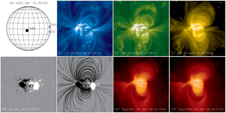
Figure 1: Images from active region 7999 on 1996 November 26. The upper left panel shows the position of the active region and the region of interest that was extracted from the full-disk images. The other panels show the EIT, MDI, and SXT images, as well as selected field lines from the potential field extrapolation. Note that the extrapolation is computed using a larger field of view than is shown so that the field lines close properly.

For each active region dataset we processed the available EIT and SXT data using the standard software and extracted a $512\arcsec\times 512\arcsec$ field of view centered on the NOAA active region coordinates rotated to the time of the image. An example set of active region observations is shown in Figure 1.

For each magnetogram we determined the total unsigned magnetic flux in the region of interest by summing all of the pixels with magnetic field strengths between 50 and 500 G and multiplying by the area per pixel. The upper limit on the fluxes under consideration allows us to exclude magnetic field lines originating in sunspots, which are known to be faint in X-rays (see Golub & Pasachoff 1997; Schrijver et al. 2004; Fludra & Ireland 2003). The lower limit excludes most quiet Sun fields from the analysis.

To compute the intensities in the EIT images we summed over all pixels with an intensity greater than twice the quiet Sun average (see Warren 2005). The use of an intensity threshold excludes the contribution of quiet Sun emission from the total EIT intensity. The difference between the total intensity above the threshold and the total intensity in the field of view is only significant for the smaller active regions. For the largest active regions the brightest pixels dominate the total intensity.

For SXT the quiet Sun contribution is generally negligible so we simply sum over all of the image to compute the total intensity. Note that our approach differs from that of Fisher et al. (1998) who converted the observed SXT fluxes to 1–300 Å luminosities ($L_{X}$) by assuming a temperature of 3 MK. Since we are able to compute the SXT and EIT intensities directly from our models we have not attempted to determine luminosities for these active regions and instead rely on the total intensity. The luminosity and the total intensities in the images are closely related and we use the two terms interchangeably. The total unsigned magnetic fluxes ($\Phi$), the magnetic area ($A_{\Phi}$), and total intensities for each active region are summarized in Table 1. Plots of total active region intensity as a function of the total unsigned magnetic flux for SXT AlMg, EIT 284 Å, 195 Å, and 171 Å are shown in Figures 2 and 3.

To facilitate comparisons between the observations and the data we fit both the simulated and observed intensities to a function of the form

$$I_{\lambda}=a_{\lambda}\Phi^{b_{\lambda}}.$$ (1)

For the SXT AlMg and Al.1 observations we find values for $b_{\lambda}$ of about 1.6. This is somewhat larger than the value of $1.19\pm 0.04$ found by Fisher et al. (1998) for the X-ray luminosity and the value of $1.27\pm 0.05$ found by Fludra & Ireland (2003) for observations of Fe XVI. The results for $b_{\lambda}$ from our fits to the EIT 171, 195, and 284 Å observations are 0.9, 0.9, and 1.08, and they differ somewhat from the value of 1.06 determined for Mg X by Schrijver (1987). The source of these differences are unclear, but they may be due to differences in methodology. Fisher et al. (1998), for example, did not use thresholds to compute the total unsigned magnetic flux. Differences in the temperature of formation of the emission may also play a role in these discrepancies.

We also calculate the linear correlation between $\log I_{\lambda}$ and $\log\Phi$ for each observed wavelength. The correlation coefficients are uniformly high (0.91–0.97) and are similar to those presented by Schrijver (1987). Fisher et al. (1998) found a somewhat smaller correlation, 0.83, between $\log L_{X}$ and $\log\Phi$.

3 Modeling

To model the topology of these active regions we use potential field extrapolations. Such simple models ignore the presence of currents in the active regions and undoubtedly oversimplify the magnetic topology. Our goal, however, is not to reproduce the exact morphology of the active regions, rather, we are primarily interested in the total intensity from the region of interest. Thus we only need to have a reasonable estimate of the loop lengths. Furthermore, Fisher et al. (1998) have shown that measurements of the large scale currents in active regions determined from vector magnetograms do not appear to provide any additional information on active region intensities.

For each active region we compute field lines for every pixel, positive and negative, in the MDI magnetogram that has a magnitude between 50 and 500 G. We then remove all of the field lines that share footpoints. For each selected field line we calculate a solution to the time-independent hydrodynamic loop equations with constant cross-section using a numerical code written by Aad van Ballegooijen (e.g., Hussain et al. 2002; Schrijver & van Ballegooijen 2005). The use of loops with constant cross section is based on the analysis of soft X-ray and EUV loops presented by Klimchuk et al. (1992) and Watko & Klimchuk (2000).

To couple the extrapolated field lines and the numerical hydro code we must make some additional assumptions. The field lines originate at the solar photosphere where the plasma temperature is approximately 4,000 K. The boundary condition for the hydro code, however, is set at 20,000 K, which corresponds to the top of the chromosphere. Close et al. (2003) have shown that in the quiet Sun a significant fraction of the field lines close at heights below 2.5 Mm, a typical chromospheric height. Thus if we were to ignore the mismatch between the base of the field line and the boundary condition on the hydro code we are likely to significantly overestimate the amount of flux that contributes to coronal heating. To account for this we use the portion of the field line above 2.5 Mm in computing the solution to the hydrostatic equations. Field lines that do not reach this height are not included in our simulations.

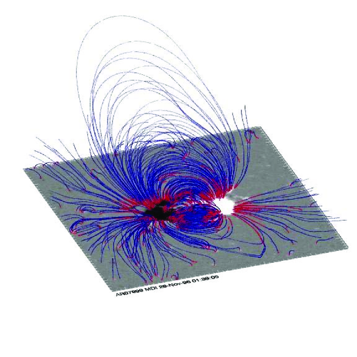
Figure 4: Selected field lines from the potential field extrapolation of AR7999 observed on 1996 November 26. The chromospheric sections of the field lines are shown in red, the coronal sections are shown in blue. Only 1 of every 3 field lines is shown.

Our procedure for using the potential field extrapolation is illustrated in Figure 4. Here the coronal portion of the field lines are shown in blue and the chromospheric part is shown in red. Note that on the Sun the chromospheric region is likely to be more radial than it appears in our potential field extrapolation.

Our volumetric heating rate is taken to be of the form

$$\epsilon_{H}=\epsilon_{0}\left(\frac{\bar{B}}{\bar{B}_{0}}\right)^{\alpha}\left(\frac{L_{0}}{L}\right)^{\beta},$$ (2)

where $\bar{B}$ is the field strength averaged along the field line, and $L$ is the total loop length. Some authors (e.g., Schrijver et al. 2004) use the footpoint field strength to parameterize the heating rate and we will discuss the implications of our parameterizations later in the paper. The parameters $\bar{B}_{0}$ and $L_{0}$ are chosen to be 76 G and 29 Mm respectively. These are the median field strengths and loop lengths determined from all of the observed active regions.

The value for $\epsilon_{0}$ is chosen so that a perpendicular field line with $\bar{B}=\bar{B}_{0}$ and $L=L_{0}$ has an apex temperature of 4 MK. The value for $\epsilon_{0}$ is 0.0492 erg cm^-3 s^-1. This choice does not set the peak temperature in the differential emission measure. The distribution of temperatures and densities in the active region depends on the distribution of magnetic field strengths and loop lengths and is difficult to relate to the choice of $\epsilon_{0}$. We will discuss the significance of $\epsilon_{0}$ later in the paper.

Once the solutions to the loop equation are computed we calculate the expected response in the various SXT and EIT channels. Note that we compute the radiative losses and instrumental responses consistently using version 5 of the CHIANTI atomic data base (e.g., Dere et al. 1997). For these calculations we assume a pressure of $10^{15}$ K cm^-3 and coronal abundances (Feldman et al., 1992). A discussion of the EIT instrumental response is given in Brooks & Warren (2005).

We have simulated EIT and SXT intensities for each of the 26 active regions using $\alpha$ and $\beta$ equal to 0, 1, and 2, for a total of 9 different heating functions. This range of values is motivated by the review of coronal heating theories by Mandrini et al. (2000). Plots of the simulated total intensities in the SXT AlMg channel as a function of total unsigned magnetic flux are shown in Figure 2. In all cases the solutions to the static models predict SXT intensities that are too large and a filling factor is needed to bring the simulated intensities into better agreement with the observations. Here we use the median ratio between the simulated and observed SXT AlMg intensities as the filling factor.

The filling factors range from less than 1% to slightly less about 30%. Filling factors are generally needed to model SXT active region emission using static heating (e.g., Porter & Klimchuk 1995). Note, however, that in our case the filling factor accounts for both the possibility of sub-resolution structures and the possibility that not all of the field lines in an active region are heated at a given time. Thus our active region filling factors are likely to be somewhat less than the filling factor that would be derived from the analysis of an individual loop.

Inspection of the simulation results for SXT AlMg, which are presented in Figure 2, show that only those cases with $\alpha=1$ $(\epsilon_{H}\sim\bar{B})$ are consistent with the observed SXT flux-intensity relationships. For $\alpha=0$ the simulated relationship is too shallow, leading to simulated intensities that are too high for the smallest magnetic fluxes and too low for the largest magnetic fluxes. The $\alpha=2$ cases, in contrast, yield a simulated curve that is too steep. The results for the SXT Al.1 filter, which are not shown, are very similar to those for the AlMg filter.

The observational and numerical results presented in Figure 2 show that the modeled flux-intensity relationships for the SXT AlMg filter are not sensitive to the dependence of the heating rate on the loop length. The $\alpha=1$, $\beta=0$, 1, and 2 cases all yield similar results for both the power-law fit of the total active region intensity to the total magnetic flux as well as for the correlation between these two parameters. This result also applies to the other high temperature emission that we have investigated, including the SXT Al.1, Al12, and Be119 filters. Thus it appears that the observed flux-intensity relationships for high temperature emission only partially constrain theories of coronal heating.

The simulated and observed flux-intensity relationships determined for EIT for the $\alpha=1$ cases, which provide the best fits to the SXT observations, are shown in Figure 3. To calculate these fluxes we have used the filling factor determined from the analysis of the SXT AlMg observations. It is clear from these comparisons that the $\beta=1$ and $\beta=2$ cases provide similar agreement, although there are some discrepancies for the EIT 284 Å channel.

The modeling of the flux-intensity relationships derived from the SXT and EIT data appears to identify the $\alpha=1$, $\beta=0$ case as not being consistent with the observations. Our choice for $\epsilon_{0}$ in Equation 2, however, was not well motivated. We have run several additional simulations to evaluate the impact of changing $\epsilon_{0}$ on the modeled intensities. As one would expect, we find that larger values of $\epsilon_{0}$ lead to higher temperatures and densities and larger intensities in the SXT channels. This necessitates the use of smaller filling factors to match the observed SXT intensities. The intensities in the EIT channels also rise with increasing energy input. This rise, however, is not as rapid as the rise in the SXT intensity and the ratio of EIT to SXT intensity actually falls with increasing $\epsilon_{0}$. Thus for larger values of $\epsilon_{0}$ the computed EIT intensities are all systematically smaller than what is observed. For smaller values of $\epsilon_{0}$ the computed EIT intensities become relatively larger. Thus the simulated intensities for the $\beta=0$ case could be brought into somewhat closer agreement with the observations for a smaller value of $\epsilon_{0}$.

While some of the comparisons between the simulated and observed EIT intensities shown in Figure show good agreement, there are no simulation parameters for which all of the computed intensities are in complete agreement with the observations. To investigate the source of these discrepancies we have computed synthetic SXT and EIT images for all of the heating functions that we have considered. To represent the intensities calculated along a field line in three dimensions we assume that the intensity at any point in space is related to the intensity on the field line by

$$I(x,y,z)=kI(x_{0},y_{0},z_{0})\exp\left[-\frac{\Delta^{2}}{2\sigma_{r}^{2}}\right]$$ (3)

where $\Delta^{2}=(x-x_{0})^{2}+(y-y_{0})^{2}+(z-z_{0})^{2}$ and $2.355\sigma_{r}$, the FWHM, is set equal to the assumed diameter of the flux tube. A normalization constant ($k$) is introduced so that the integrated intensity of over all space is equal to the intensity integrated along the field line. This approach for the visualization is based on the method used in Karpen et al. (2001).

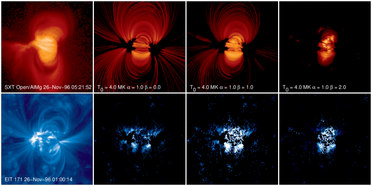
Figure 5: Synthetic SXT AlMg and EIT 171 Å images for AR7997. Images for the $\alpha=1$, $\beta=0$, 1, and 2 cases are shown. The images are displayed with the same scalings used in Figure 1. Note that the synthetic images have not been convolved with the instrumental point spread functions.

Example images for AR 7999 are shown in Figure 5. These comparisons suggest that the distribution of intensities offer important additional constraints on the modeling. For example, the SXT AlMg images for the $\alpha=1$, $\beta=2$ case show that while the total intensities are generally consistent with the observations, the distribution of these intensities is not consistent with the SXT data. For this set of parameters all of the simulated emission is concentrated in the shortest loops. For the $\alpha=1$, $\beta=0$ case the longer loops appear to be too bright relative to the observations. Qualitatively, the $\alpha=1$, $\beta=1$ parameters appear to provide the best match between the simulation and the observations.

At the lower temperatures imaged with EIT, however, the differences between the modeled active regions and the observations are dramatic. The computed images are dominated by the transition region emission of the hot loops. This emission is often referred to as the “moss” (e.g., Berger et al. 1999; Fletcher & de Pontieu 1999; Martens et al. 2000). The observed images, in contrast, are a combination of moss emission and emission from loops. The inability of static models to reproduce the loops observed in the EUV is well documented (e.g., Lenz et al. 1999; Aschwanden et al. 2001; Winebarger et al. 2003). The absence of EUV loops in active regions simulated with static models has also been noted by Schrijver et al. (2004).

From these visualizations we also see that the computed moss intensities are too large to be consistent with the observations. Such large discrepancies are found in all of the active regions we have simulated and are also present for the EIT 195 Å and 284 Å channels. Thus the reasonable agreement between the computed and observed total intensities shown in Figure 3 is misleading and highlights a potential pitfall in relying on integrated intensities.

One of the essential assumptions in our modeling is that the loops have a constant cross-section. An analysis of individual loops supports this assumption (Klimchuk et al., 1992; Watko & Klimchuk, 2000). Other simulation work has considered expanding loops (e.g., Schrijver et al. 2004). We have rerun the active region simulations assuming that the loops have cross-sectional areas that expand proportional to $1/B(s)$. The same volumetric heating rate given by Equation 2 is used in these simulations. The resulting solutions to the loop equations are generally similar, but not identical, to the solutions with constant cross-section (e.g., Aschwanden & Schrijver 2002). The primary difference is in the emission measure. The expanded cross-section at the top of the loop tends to enhance the contribution of the high temperature emission, since the temperatures are generally highest at the loop apex and the loop expansion leads to larger emission measures there. Thus the simulated SXT emission is typically larger with expanding cross sections than in the corresponding constant cross section case, and a smaller filling factor is needed to bring the calculated intensities into agreement with the observations. The modeled flux-intensity relationships for the expanding cross-section case are very similar to those shown in Figure 2

The moss emission from the hot SXT loops that is imaged by EIT occurs low in the loop and the calculated EIT intensities are not impacted significantly by the flux tube expansion. Thus the modeled EIT intensities become smaller when a smaller filling factor is used and can be brought into closer agreement with the data. With this reduction, the computed moss intensities become much smaller. As shown in Figure 6, however, the total intensities computed assuming expanding flux tubes are a factor of 20 or more below the observed intensities. We also note that the parameters derived from the fits of the total intensity to the total unsigned flux differ significantly from those determined from the simulations with constant cross section.

4 Summary and Discussion

We have presented extensive numerical simulations of the SXT and EIT emission observed in solar active regions. This modeling, which is based on potential field extrapolations and solutions to the hydrostatic loop equations, indicates that a volumetric heating rate that scales as $\bar{B}/L$ is the most consistent with the observations. Thus these simulation results offer significant constraints on theories of coronal heating.

Our analysis, however, has identified several weaknesses in this approach to modeling active region emission. We find that the computed SXT emission for $\alpha=1$, $\beta=0$ ($\epsilon_{H}\sim\bar{B}$) and $\beta=2$ ($\epsilon_{H}\sim\bar{B}/L^{2}$) are also consistent with the observed SXT flux-intensity relationships. It is only in combination with visualizations of the active region emission that we find that these simulations offer strong constraints on the volumetric heating rate.

Furthermore, from visualizations of the cooler emission imaged with EIT we find significant differences between the observations and the simulations. The simulated EIT images lack the loop structures that are found in the observations. The computed moss intensities are also much larger than what is observed on the Sun. We have found that it is possible to bring the moss intensities into closer agreement with the observations by allowing the allowing the flux tubes to expand proportional to $1/B(s)$. In this case, however, the integrated EIT intensities fall well below what is observed.

Many of our simulation results are consistent with the full Sun visualizations presented by Schrijver et al. (2004). Using potential field extrapolations and static heating models they find that a energy flux which scales as $F_{H}\sim B_{0}/L$, where $B_{0}$ is the footpoint field strength, is consistent with the SXT and EIT images. Schrijver & Title (2005) also find that this form for the heating flux is consistent with the flux-luminosity relationship derived from observations of other cool dwarf stars. In our work we have used $\bar{B}$, the magnetic field averaged along a field line, in our parameterization of the volumetric heating rate. From our sample of over 100,000 field lines we find that $\bar{B}\sim B_{0}/L$, which implies

$$\epsilon_{H}\sim F_{H}/L\sim B_{0}/L^{2}\sim\bar{B}/L,$$ (4)

bringing our results into agreement with those of Schrijver et al. (2004).

In our simulations we require a filling factor of about 30% to bring the modeled and observed SXT fluxes into agreement for the $\alpha=1$, $\beta=1$ case. Schrijver et al. (2004) and Schrijver & Title (2005) are able to reproduce the observed soft X-ray fluxes without the need for a filling factor. We have traced this discrepancy to the differences in the spatial resolution of the magnetograms. Schrijver et al. (2004) use Carrington maps with a 1^∘ resolution while we use MDI magnetograms with approximately 2$\arcsec$ resolution. Using lower spatial resolution removes much of the small-scale fields that would close in the chromosphere. We find that if we bin our magnetograms to much lower spatial resolution we obtain a filling factor much closer to 1.

We feel that our method for removing the chromospheric loops from the extrapolation of high resolution magnetograms is likely to provide for more realistic simulated images. It is clear, however, that this type of active region modeling is in its earliest stages and considerable approximations are involved. Given the complexity of the solar atmosphere and the limitations of our calculations we are not confident in many of the simulation details, such as the magnitude of the filling factor. Additionally, we note that the filling factor is dependent on the assumed value for $\epsilon_{0}$, which is not well constrained by these observations. The simulation of active regions with more complete data, such as SXT images in thicker filters, will provide better constraints on this parameter.

So where does this leave us? If we take the position that the high temperature emission imaged by SXT represents the most important signature of the coronal heating mechanism, then we can conclude that static models adequately reproduce high temperature coronal emission and that the volumetric heating rate must scale approximately as $\bar{B}/L$. Schrijver et al. (2004) have argued that of all the coronal heating models presented in the summary by Mandrini et al. (2000), their model 4, the field-braiding reconnection model of Parker (1983), agrees best with this parameterization. These comparisons are limited, however, by the approximate nature of the scaling laws that are used to represent the model predictions. Theoretical models that make more quantitative predictions about the volumetric heating rate are sorely needed.

The inability of static models to account for much of the active region emission at the 1–2, MK emission imaged by EIT is troubling. Recent work has shown that the active region loops observed at these lower temperatures are often evolving (Winebarger et al., 2003). Simulation results suggest that the observational properties of these loops can be understood using dynamical models where the loops are heated impulsively and are cooling (Warren et al., 2003; Warren et al., 2002). There is also some evidence that the densities in the quiet Sun may be too large to be accounted for by static heating models (Warren & Warshall, 2002). We conjecture that dynamic heating will ultimately be required to model the high temperature SXT emission observed in solar active regions. At present, however, the observational evidence at these temperatures is consistent with static heating.

Figure 2: Simulated and observed total SXT AlMg intensities as a function of the total unsigned magnetic flux. Each panel represents the results from a single combination of $\alpha$ and $\beta$. The observed intensities are repeated in each panel. A filling factor is used to scale the simulated SXT intensities to match the observed intensities as closely as possible. The parameters for the power-law fit (Equation 1) are given in each panel. The correlation between $\log I_{\lambda}$ and $\log\Phi$ is also given.

Figure 3: Simulated and observed total EIT 284, 195, and 171 Å intensities as a function of the total unsigned magnetic flux. The filling factor is taken from the SXT AlMg results. Only the $\alpha=1$ cases are shown. Each row corresponds to a single EIT wavelength. Each column corresponds to a single value for $\beta$.

Figure 6: Simulated and observed total EIT 284, 195, and 171 Å intensities as a function of the total unsigned magnetic flux. These calculations assume that the flux tube areas expand with distance along the loop. The filling factors are taken from the SXT AlMg results, which are not shown.

Table 1: Summary of Active Region Observations

NOAA	MDI Time	$\Phi$ (Mx)	$A_{\Phi}$ (cm2)	$I_{ALMG}$	$I_{171}$	$I_{195}$	$I_{284}$
7982	9-Aug-1996 14:24:04	2.23(21)	1.86(19)	1.52(05)	5.41(06)	3.40(06)	1.65(05)
7999	26-Nov-1996 01:39:05	1.13(22)	6.62(19)	3.76(06)	6.39(06)	5.27(06)	5.22(05)
8032	16-Apr-1997 09:40:04	3.07(21)	2.33(19)	4.60(05)	6.20(06)	3.61(06)	2.22(05)
8055	23-Jun-1997 14:24:05	2.03(21)	1.88(19)	8.36(04)	5.72(06)	3.22(06)	1.55(05)
8060	9-Jul-1997 09:36:04	2.12(21)	1.50(19)	2.00(05)	5.62(06)	2.76(06)	1.37(05)
8096	19-Oct-1997 17:35:03	3.06(21)	2.56(19)	4.56(05)	5.98(06)	3.40(06)	1.93(05)
8170	28-Feb-1998 01:20:04	1.22(21)	1.33(19)	2.57(04)	5.28(06)	2.47(06)	1.15(05)
8174	10-Mar-1998 22:24:03	4.93(21)	4.30(19)	—	5.48(06)	3.83(06)	2.70(05)
8179	15-Mar-1998 16:00:03	2.19(22)	1.38(20)	—	9.83(06)	7.61(06)	9.12(05)
8218	12-May-1998 14:24:04	1.53(22)	1.11(20)	1.47(06)	5.94(06)	4.60(06)	4.94(05)
8542	17-May-1999 12:48:03	7.16(21)	6.01(19)	3.59(05)	6.56(06)	4.44(06)	3.49(05)
8603	30-Jun-1999 06:27:02	2.52(22)	1.53(20)	4.99(06)	1.21(07)	8.11(06)	1.06(06)
8636	23-Jul-1999 17:36:02	3.86(22)	2.50(20)	—	1.23(07)	9.73(06)	1.31(06)
8793	10-Dec-1999 17:35:03	8.15(21)	6.50(19)	—	4.82(06)	3.36(06)	3.78(05)
8807	24-Dec-1999 03:11:02	3.04(22)	1.98(20)	6.95(06)	1.33(07)	9.53(06)	1.20(06)
8882	27-Feb-2000 14:27:02	1.52(22)	9.99(19)	3.93(06)	7.65(06)	5.65(06)	6.46(05)
8921	26-Mar-2000 17:35:02	2.02(22)	1.38(20)	3.63(06)	9.12(06)	7.20(06)	9.20(05)
9087	19-Jul-2000 22:23:01	3.37(22)	2.15(20)	1.57(07)	1.04(07)	8.13(06)	1.23(06)
9169	24-Sep-2000 08:00:01	5.13(22)	2.95(20)	1.25(07)	1.68(07)	1.26(07)	1.88(06)
9182	8-Oct-2000 19:11:02	1.51(22)	1.16(20)	1.12(06)	8.28(06)	6.75(06)	7.61(05)
9228	12-Nov-2000 03:11:02	3.25(21)	3.29(19)	2.47(05)	3.70(06)	2.86(06)	2.59(05)
9329	2-Feb-2001 11:11:01	6.55(21)	5.38(19)	5.05(05)	5.80(06)	4.52(06)	4.43(05)
9477	29-May-2001 11:12:02	4.06(21)	3.92(19)	1.43(05)	5.37(06)	2.89(06)	1.75(05)
9484	4-Jun-2001 14:27:01	1.07(22)	8.58(19)	1.77(06)	5.95(06)	4.55(06)	5.41(05)
9682	31-Oct-2001 06:27:02	2.61(22)	1.60(20)	9.31(06)	1.02(07)	7.55(06)	9.65(05)
9710	22-Nov-2001 09:35:02	1.16(22)	9.04(19)	1.85(06)	8.14(06)	6.42(06)	7.54(05)

References

- Aschwanden et al. (2000) Aschwanden, M. J., Nightingale, R. W., & Alexander, D. 2000, ApJ, 541, 1059
- Aschwanden & Schrijver (2002) Aschwanden, M. J., & Schrijver, C. J. 2002, ApJS, 142, 269
- Aschwanden et al. (2001) Aschwanden, M. J., Schrijver, C. J., & Alexander, D. 2001, ApJ, 550, 1036
- Berger et al. (1999) Berger, T. E., de Pontieu, B., Schrijver, C. J., & Title, A. M. 1999, ApJ, 519, L97
- Brooks & Warren (2005) Brooks, D. H., & Warren, H. P. 2005, ApJS
- Close et al. (2003) Close, R. M., Parnell, C. E., Mackay, D. H., & Priest, E. R. 2003, Sol. Phys., 212, 251
- Delaboudinière et al. (1995) Delaboudinière, J.-P., et al. 1995, Sol. Phys., 162, 291
- Dere et al. (1997) Dere, K. P., Landi, E., Mason, H. E., Monsignori Fossi, B. C., & Young, P. R. 1997, A&AS, 125, 149
- Feldman et al. (1992) Feldman, U., Mandelbaum, P., Seely, J. F., Doschek, G. A., & Gursky, H. 1992, ApJS, 81, 387
- Fisher et al. (1998) Fisher, G. H., Longcope, D. W., Metcalf, T. R., & Pevtsov, A. A. 1998, ApJ, 508, 885
- Fletcher & de Pontieu (1999) Fletcher, L., & de Pontieu, B. 1999, ApJ, 520, L135
- Fludra & Ireland (2003) Fludra, A., & Ireland, J. 2003, in The Future of Cool-Star Astrophysics: 12th Cambridge Workshop on Cool Stars , Stellar Systems, and the Sun (2001 July 30 - August 3), eds. A. Brown, G.M. Harper, and T.R. Ayres, (University of Colorado), 2003, p. 220-229., 220
- Golub & Pasachoff (1997) Golub, L., & Pasachoff, J. M. 1997, The Solar Corona (The Solar Corona, by Leon Golub and Jay M. Pasachoff, ISBN 0521480825. Cambridge, UK: Cambridge University Press, September 1997.)
- Hussain et al. (2002) Hussain, G. A. J., van Ballegooijen, A. A., Jardine, M., & Collier Cameron, A. 2002, ApJ, 575, 1078
- Karpen et al. (2001) Karpen, J. T., Antiochos, S. K., Hohensee, M., Klimchuk, J. A., & MacNeice, P. J. 2001, ApJ, 553, L85
- Klimchuk et al. (1992) Klimchuk, J. A., Lemen, J. R., Feldman, U., Tsuneta, S., & Uchida, Y. 1992, PASJ, 44, L181
- Lenz et al. (1999) Lenz, D. D., Deluca, E. E., Golub, L., Rosner, R., & Bookbinder, J. A. 1999, ApJ, 517, L155
- Lundquist et al. (2004) Lundquist, L. L., Fisher, G. H., McTiernan, J. M., & Régnier, S. 2004, in ESA SP-575: SOHO 15 Coronal Heating, ed. R. W. Walsh, J. Ireland, D. Danesy, & B. Fleck, 306
- Mandrini et al. (2000) Mandrini, C. H., Démoulin, P., & Klimchuk, J. A. 2000, ApJ, 530, 999
- Martens et al. (2000) Martens, P. C. H., Kankelborg, C. C., & Berger, T. E. 2000, ApJ, 537, 471
- Parker (1983) Parker, E. N. 1983, ApJ, 264, 642
- Pevtsov et al. (2003) Pevtsov, A. A., Fisher, G. H., Acton, L. W., Longcope, D. W., Johns-Krull, C. M., Kankelborg, C. C., & Metcalf, T. R. 2003, ApJ, 598, 1387
- Porter & Klimchuk (1995) Porter, L. J., & Klimchuk, J. A. 1995, ApJ, 454, 499
- Rosner et al. (1978) Rosner, R., Tucker, W. H., & Vaiana, G. S. 1978, ApJ, 220, 643
- Scherrer et al. (1995) Scherrer, P. H., et al. 1995, Sol. Phys., 162, 129
- Schrijver (1987) Schrijver, C. J. 1987, A&A, 180, 241
- Schrijver et al. (2004) Schrijver, C. J., Sandman, A. W., Aschwanden, M. J., & DeRosa, M. L. 2004, ApJ, 615, 512
- Schrijver & Title (2005) Schrijver, C. J., & Title, A. M. 2005, ApJ, 619, 1077
- Schrijver & van Ballegooijen (2005) Schrijver, C. J., & van Ballegooijen, A. A. 2005, ApJ, 630, 552
- Tsuneta et al. (1991) Tsuneta, S., et al. 1991, Solar Phys., 136, 37
- Warren (2005) Warren, H. P. 2005, ApJS, 157, 147
- Warren & Warshall (2002) Warren, H. P., & Warshall, A. D. 2002, ApJ, 571, 999
- Warren et al. (2002) Warren, H. P., Winebarger, A. R., & Hamilton, P. S. 2002, ApJ, 579, L41
- Warren et al. (2003) Warren, H. P., Winebarger, A. R., & Mariska, J. T. 2003, ApJ, 593, 1174
- Watko & Klimchuk (2000) Watko, J. A., & Klimchuk, J. A. 2000, Sol. Phys., 193, 77
- Winebarger et al. (2003) Winebarger, A. R., Warren, H. P., & Mariska, J. T. 2003, ApJ, 587, 439
- Winebarger et al. (2003) Winebarger, A. R., Warren, H. P., & Seaton, D. B. 2003, ApJ, 593, 1164