Microlensing Sensitivity to Earth-mass Planets in the Habitable Zone

Abstract

Microlensing is one of the most powerful methods that can detect extrasolar planets and a future space-based survey with a high monitoring frequency is proposed to detect a large sample of Earth-mass planets. In this paper, we examine the sensitivity of the future microlensing survey to Earth-mass planets located in the habitable zone. For this, we estimate the fraction of Earth-mass planets that will be located in the habitable zone of their parent stars by carrying out detailed simulation of microlensing events based on standard models of the physical and dynamic distributions and the mass function of Galactic matter. From this investigation, we find that among the total detectable Earth-mass planets from the survey, those located in the habitable zone would comprise less than 1% even under a less-conservative definition of the habitable zone. We find the main reason for the low sensitivity is that the projected star-planet separation at which the microlensing planet detection efficiency becomes maximum (lensing zone) is in most cases substantially larger than the median value of the habitable zone. We find that the ratio of the median radius of the habitable zone to the mean radius of the lensing zone is roughly expressed as $d_{\rm HZ}/r_{\rm E}\sim 0.2(m/0.5\ M_{\odot})^{1/2}$.

1. Introduction

Since the first detection by using the pulsar timing method (Wolszczan & Frail, 1992), extrasolar planets have been and are going to be detected by using various techniques including the radial velocity technique (Mayor & Queloz, 1995; Marcy & Butler, 1996), transit method (Struve, 1952), astrometric technique (Sozzetti, 2005), direct imaging (Angel, 1994; Stahl & Sandler, 1995), and microlensing (Mao & Paczyński, 1991; Gould & Loeb, 1992). See the reviews of Perryman (2000, 2005).

The microlensing signal of a planet is a short-duration perturbation to the smooth standard light curve of the primary-induced lensing event occurring on a background source star. The planetary lensing signal induced by a giant planet with a mass equivalent to that of the Jupiter lasts for a duration of $\sim 1$ day, and the duration decreases in proportion to the square root of the mass of a planet, reaching several hours for an Earth-mass planet. Once the signal is detected and analyzed, it is possible to determine the planet/primary mass ratio, $q$, and the projected primary-planet separation, $s$, in units of the Einstein ring radius $r_{\rm E}$, which is related to the mass of the lens, $m$, and distances to the lens and source, $D_{L}$ and $D_{S}$, by

$$r_{\rm E}\simeq 4.9\ {\rm AU}\left({m\over 0.5\ M_{\odot}}\right)^{1/2}\left({D_{L}\over 6\ {\rm kpc}}\right)^{1/2}\left(1-{D_{L}\over D_{S}}\right)^{1/2}.$$ (1)

Currently, several experiments are going underway to search for planets by using the microlensing technique and two robust detections of Jupiter-mass planets were recently reported by Bond et al. (2004) and Udalski et al. (2005). In addition, a future space-based survey with the capability of continuously monitoring stars at high cadence by using very large format imaging cameras is proposed to detect a large sample of Earth-mass planets (Bennett & Rhie, 2002).

The microlensing technique has various advantages over other methods. First, microlensing is sensitive to lower-mass planets than most other methods and it is possible, in principle, to detect Earth-mass planets from ground-based observations with adequate monitoring frequency and photometric precision (Gould, Gaudi, & Han, 2004). Second, a large sample of planets, especially low-mass terrestrial planets, will be detected at high S/N with the implementation of future lensing surveys, and thus the microlensing technique will be able to provide the best statistics of Galactic population of planets. Third, the planetary lensing signal can be produced by the planet itself, and thus the microlensing technique is the only proposed method that can detect and characterize free-floating planets (Bennett & Rhie, 2002; Han et al., 2005). Fourth, the microlensing technique is distinguished from other techniques in the sense that the planets to which it is sensitive are much more distant than those found with other techniques and the method can be extended to search for planets located even in other galaxies (Covone et al., 2000; Baltz & Gondolo, 2001).

In addition to the detections of planets, the habitability of the detected planets is of great interest. One basic condition for the habitability is that planets should be located at a suitable distance from their host stars. Then, a question is whether a significant fraction of planets to be detected by future lensing surveys would be in the lensing zone. If the planets in the habitable zone comprise a significant fraction of the total microlensing sample of planets, a statistical analysis on the frequency of terrestrial planets in the habitable zone would be possible under some sorts of assumptions about the shape and inclination of the planetary orbit around host stars. In this paper, we examine the sensitivity of future lensing surveys to Earth-mass planets located in the habitable zone by carrying out detailed simulation of Galactic microlensing events based on the standard models of the physical and dynamic distributions and the mass function of Galactic matter. The sensitivities to habitable-zone planets of other planet search methods were discussed by Gould, Pepper, & DePoy (2003) (transit method), Gould, Ford, & Fischer (2003) (astrometric method), and Sozzetti et al. (2002) (space interferometry).

The paper is organized as follows. In § 2, we briefly describe the basics of planetary microlensing. In § 3, we describe the procedure of the simulation of Galactic microlensing events produced by lenses with Earth-mass planet companions. We then describe the procedure of estimating the fraction of planets located in the habitable zone among the total number of detectable Earth-mass planets based on the planetary lensing events produced by the simulation. In § 4, we present the results of the simulation and discuss about the results. We conclude in § 5.

2. Basics of Planetary Microlensing

Planetary lensing is an extreme case of binary lensing with a very low-mass companion. Because of the very small mass ratio, planetary lensing behavior is well described by that of a single lens of the primary for most of the event duration. However, a short-duration perturbation can occur when the source star passes the region around caustics.

The caustic is an important feature of binary lensing and it represents the source position at which the lensing magnification of a point source becomes infinite. The caustics of binary lensing form a single or multiple closed figures where each of which is composed of concave curves (fold caustics) that meet at cusps. For a planetary case, there exist two sets of disconnected caustics. One small ‘central’ caustic is located close to the primary lens, while the other bigger ‘planetary’ caustic(s) is (are) located away from the primary at the position with a separation vector from the primary lens of

$${\bf r}={\bf s}\left(1-{1\over s}\right)^{2},$$ (2)

where ${\bf s}$ is the position vector of the planet from the primary lens. Then, the caustics are located within the Einstein ring when the planet is located within the separation range of $0.6\lesssim s\lesssim 1.6$, which is often referred as the ‘lensing zone’. The number of the planetary caustics is one or two depending on whether the planet lies outside ($s>1$) or inside ($s<1$) the Einstein ring.

The size of the caustic, which is directly proportional to the planet detection efficiency, is dependent on both $q$ and $s$. Under perturbative approximation (when $q\ll 1$ and $|s-1|\gg q$), the sizes of the central ($\Delta r_{\rm cc}$) and planetary ($\Delta r_{\rm pc}$) caustics as measured by the width along the star-planet axis are represented, respectively, by

$${\Delta r_{\rm cc}\over r_{\rm E}}\simeq{4q\over(s-s^{-1})^{2}}\rightarrow\cases{4qs^{-2},&for $s>1$,\cr 4qs^{2},&for $s<1$,\cr}$$ (3)

and

$${\Delta r_{\rm pc}\over r_{\rm E}}\simeq\cases{4q^{1/2}[s(s^{2}-1)^{1/2}]^{-1}\rightarrow 4q^{1/2}s^{-2},&for $s>1$,\cr 2q^{1/2}(\kappa_{0}-\kappa_{0}^{-1}+\kappa_{0}s^{-2})\cos\theta_{0}\rightarrow 1.3q^{1/2}s^{3},&for $s<1$,\cr}$$ (4)

where $\kappa(\theta)=\{[\cos 2\theta\pm(s^{4}-\sin^{2}2\theta)^{1/2}]/(s^{2}-1/s^{2})\}^{1/2}$, $\theta_{0}=[\pi\pm\sin^{-1}({\sqrt{3}s^{2}/2})]/2$, and $\kappa_{0}=\kappa(\theta_{0})$ (Bozza, 2000; An, 2005; Chung et al., 2005; Han, 2006). The size of the caustic becomes maximum when $s\sim 1$ and decreases rapidly as the separation becomes bigger ($\propto s^{-2}$ for both the central and planetary caustics) or smaller ($\propto s^{2}$ for the central caustic and $\propto s^{3}$ for the planetary caustic) than the Einstein ring radius. As a result, only planets located within the lensing zone have non-negligible chance of producing planetary signals.

In Figure 1, we present the variation of the total caustic size, $\Delta r_{\rm c}=\Delta r_{\rm cc}+\Delta r_{\rm pc}$, as a function of the primary-planet separation for a planetary lens system with a mass ratio of $q=10^{-5}$, which corresponds to an Earth-mass planet around a star with $0.3\ M_{\odot}$. In the figure, the dotted curve is calculated numerically while the dashed curve is computed analytically by using the formalism in equations (3) and (4). The disagreement between the two curves in the region around $s=1$ is due to the failure of the perturbative approximation in this region.

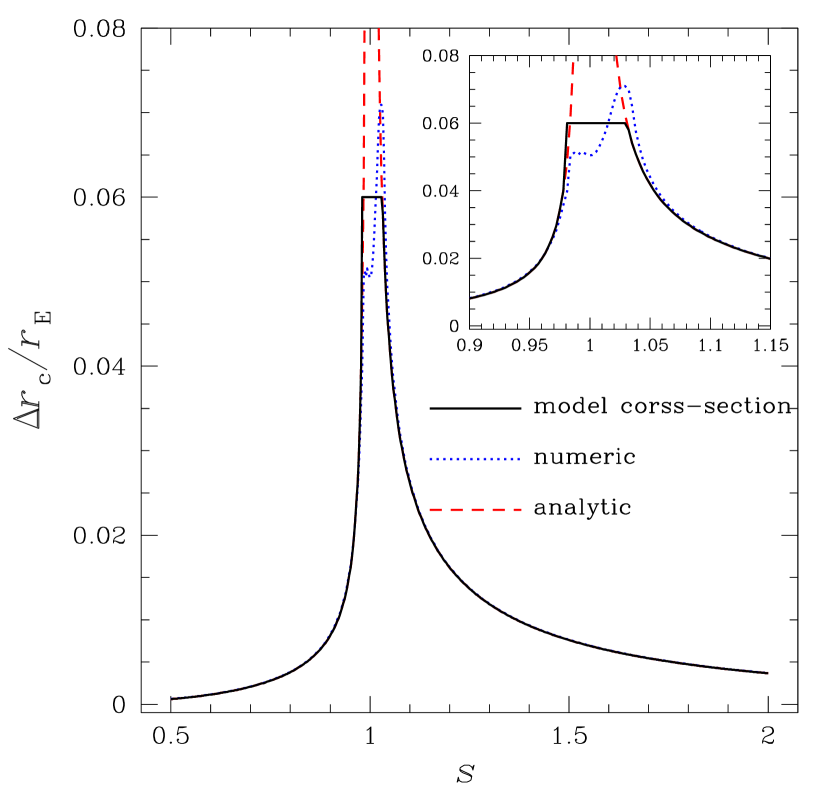
Figure 1.— The variation of the caustic size as a function of the primary-planet separation, $s$, for a planetary lens system with a mass ratio of $q=10^{-5}$. The dotted curve is calculated numerically while the dashed curve is computed by using the analytic formalism based on perturbative approximation (Eqs. [3] and [4]). The two results match very well except the region around $s=1$, where the perturbative approximation is no longer valid. The solid curve is the model adopted in our simulation as the relative planet detection efficiency as a function of $s$.

3. Simulation

To estimate the fraction of planets located in the habitable zone among the total number of Earth-mass planets detectable by future lensing surveys, we conduct detailed simulation of Galactic microlensing events. In the simulation, we assume that the survey is conducted toward the Baade’s Window field centered at the Galactic coordinates of $(l,b)=(1^{\circ},-4^{\circ})$. The absolute brightnesses of the source stars are assigned on the basis of the luminosity function of Holtzman et al. (1998) constructed by using the Hubble Space Telescope. Once the absolute magnitude is assigned, the apparent magnitude is determined considering the distance to the source star and extinction. The extinction is determined such that the source star flux decreases exponentially with the increase of the dust column density. The dust column density is computed on the basis of an exponential dust distribution model with a scale height of $h_{z}=120\ {\rm pc}$, i.e. $\propto\exp(-|z|/h_{z})$, where $z$ is the distance from the Galactic plane. We normalize the amount of extinction so that $A_{V}=1.28$ for a star located at $D_{\rm S}=8\ {\rm kpc}$ following the measurement of Holtzman et al. (1998). The proposed space-based lensing survey searching for Earth-mass planets will monitor main-sequence stars to minimize the finite-source effect, which washes out the planetary lensing signal. We, therefore, assume that the brightness range of source stars to be monitored by the survey is $18.5\lesssim V\lesssim 25.0$, which corresponds to early F to early M-type main-sequence stars.

The locations of the source stars and lens matter are allocated based on the standard mass distribution model of Han & Gould (2003). In the model, the bulge mass distribution is scaled by the deprojected infrared light density profile of Dwek et al. (1995), specifically model G2 with $R_{\rm max}=5$ kpc from their Table 2. The velocity distribution of the bulge is deduced from the tensor virial theorem and the resulting distribution of the lens-source transverse velocity is listed in Table 1 of Han & Gould (1995), specifically non-rotating barred bulge model. The disk matter distribution is modeled by a double-exponential law, which is expressed as $\rho(R,z)=\rho_{0}\exp[-(r-R_{0})/h_{R}+|z|/h_{z}]$, where $(R,z)$ is the Galactocentric cylindrical coordinates, $R_{0}=8$ kpc is the distance of the sun from the Galactic center, $\rho_{0}=0.06\ M_{\odot}\ {\rm pc}^{-3}$ is the mass density in the solar neighborhood, and $h_{R}=3.5$ kpc and $h_{z}=325$ pc are the radial and vertical scale heights. According to the models of the dynamical and physical distributions, the ratio between the rates of bulge-bulge and disk-bulge events is $\Gamma_{\rm b}:\Gamma_{\rm d}=61.8:38.2$.

We assign the lens mass based on the model mass function of Gould (2000). The model mass function is composed of stars, brown dwarfs (BDs), and stellar remnants of white dwarfs (WDs), neutron stars (NSs), and black holes (BHs). The model is constructed under the assumption that bulge stars formed initially according to a double power-law distribution of the form

$${dN\over dm}=k\left({m\over m_{\rm c}}\right)^{\gamma};\qquad\gamma=\cases{-2.0&for $m>m_{\rm c}$,\cr-1.3&for $m<m_{\rm c}$,\cr}$$ (5)

where $m_{\rm c}=0.7\ M_{\odot}$. These slopes are consistent with the observations of Zoccali et al. (2000) except that the profile is extended to a BD cutoff of $m=0.03\ M_{\odot}$. Based on this initial mass function, remnants are modeled by assuming that the stars with initial masses $1\ M_{\odot}<m<8\ M_{\odot}$, $8\ M_{\odot}<m<40\ M_{\odot}$, and $m>40\ M_{\odot}$ have evolved into WDs (with a mass $0.6\ M_{\odot}$), NSs (with a mass $13.5\ M_{\odot}$), and BHs (with a mass $5\ M_{\odot}$), respectively. Note that since we assume stars with $m>1\ M_{\odot}$ have evolved into remnants, the upper limit of the stellar lens mass is $1\ M_{\odot}$, corresponding to the turn-off star in the Galactic bulge. Then, the resulting mass fractions of the individual lens components are ${\rm stars}:{\rm BD}:{\rm WD}:{\rm NS}:{\rm BH}=62:7:22:6:3$. An important fraction of lenses are stars and thus they will contribute to the apparent brightness of the source star. We consider this by determining the lens brightness by using the mass-$M_{V}$ relation listed in Allen (2000).

For each event involved with a primary lens, we then introduce a companion of an Earth-mass planet. The location of the planet around the primary star is allocated under the assumption of a circular orbit with a power-law distribution of semi-major axes $a$, i.e. $dN_{\rm p}/da\propto a^{-\alpha}$, and random orientation of the orbital plane. There is little consensus about the power of the semi-major axis distribution. Tabachnik & Tremaine (2002) claimed $\alpha=1$ from the analysis of observed extrasolar planets detected by radial velocity surveys. The minimum mass solar nebula has surface density with $\alpha=1.5$ (Hayashi, 1995). Kuchner (2004) argued that multi-planet extrasolar planetary systems indicate $\alpha=2.0$. We, therefore, test three different powers of $\alpha=1.0$, 1.5, and 2.0. The range of the semi-major axis is $-2\leq\log(a/{\rm AU})\leq 2$, which is wide enough to cover the lensing zone of all possible lenses, and thus the exact range we consider does not affect the relative frequencies we calculate here. Once a planetary event is produced, the rate of each event is computed by

$$\Gamma_{{\rm p},i}\propto\rho(D_{\rm S})D_{\rm S}^{2}\rho(D_{\rm L})\sigma_{L}v\Delta r_{\rm c},$$ (6)

where $\rho(D)$ is the matter density along the line of sight, the factor $D_{\rm S}^{2}$ is included to account for the increase of the number of source stars with the increase of $D_{\rm S}$, $\sigma_{L}$ represents the lensing cross-section corresponding to the diameter of the Einstein ring, i.e. $\sigma_{L}=2r_{\rm E}$, and $v$ is the transverse speed of the lens with respect to the source star. The factor $\Delta r_{\rm c}$ is included to weight the planet detection efficiency by the cross-section of the planetary perturbation under the assumption that the planet detection efficiency is proportional to the caustic size. For the acceleration of the computation, we use $\Delta r_{\rm c}$ computed analytically by using the formalism derived under the perturbative approximation (Eqs. [3] and [4]) except the region where the approximation is not valid. In this region, we use the mean value of the numerical results averaged over the region (the solid curve in Fig. 1). Then, the fraction of events with planets in the habitable zone among the total number of events with detectable Earth-mass planets is calculated by

$$f_{\rm HZ}={\sum\Gamma_{{\rm p},i}(d_{\rm in}\leq a\leq d_{\rm out})\over\sum\Gamma_{{\rm p},i}},$$ (7)

where $d_{\rm in}$ and $d_{\rm out}$ are the inner and outer limits of the habitable zone, respectively. The semi-major axis is related to the projected separation by

$$a={s\over(\cos^{2}\phi+\sin^{2}\phi\cos^{2}i)^{1/2}}r_{\rm E},$$ (8)

where $\phi$ is the phase angle of the planet measured from the major axis of the apparent orbit of the planet around the host star and $i$ is the inclination angle of the orbital plane.

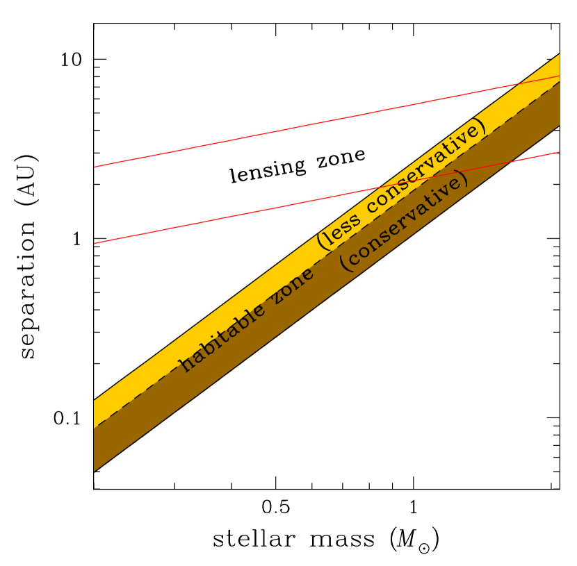
Figure 2.— The ranges of the habitable zone and lensing zone as a function of a stellar mass. For the habitable zone, the dark and light-shaded regions represent the conservative and less-conservative ranges of the habitable zone, respectively. The lensing zone is computed assuming that the distances to the lens and source star are $D_{L}=6$ kpc and $D_{S}=8$ kpc, respectively.

The habitable zone is defined as a shell region around a star within which a planet may contain liquid water on its surface. A convenient way of estimating the inner and outer limits of the habitable zone is to assume that the planet behaves as a graybody with an albedo and with perfect heat conductivity (implying that the temperature is uniform over the planet’s surface). Under this assumption, the inner and outer limits of the habitable zone are determined as

$$d_{\rm in(out)}=\left[{(1-{\cal A}_{L})L_{\star}\over 16\pi\sigma T^{4}}\right]^{1/2},$$ (9)

where $L_{\star}$ is the luminosity of the star, ${\cal A}_{L}$ is the albedo of the planet, $\sigma$ is the Stefan-Boltzmann constant, and $T$ is the radiative equilibrium temperature. In the simulation, we test two ranges of the habitable zone. For a conservative range, we adopt radiative equilibrium temperatures of $T=269$ K and $203$ K for the inner and outer limits of the habitable zone, respectively. A less-conservative range has the same inner radius as that of the conservative range, but the outer limit is defined by a lower radiative equilibrium temperature of $T=169$ K (Lopez, Schneider & Danchi, 2005). For the albedo, we choose ${\cal A}_{L}=0.2$ as a representative value of an Earth-like planet. For a sun-like star, then, the inner limit of the habitable zone is $d_{\rm in}=0.96\ {\rm AU}$ and the outer limits are $d_{\rm out}=1.69\ {\rm AU}$ and 2.43 AU for the conservative and less-conservative ranges, respectively. For the conversion of the mass of the star into the luminosity, we use the mass-luminosity relation (Allen, 2000) of

$$\log\left({L\over L_{\odot}}\right)=3.8\log\left({m\over M_{\odot}}\right)+0.08.$$ (10)

Figure 2 shows the conservative (dark-shaded region) and less-conservative (light-shaded region) ranges of the habitable zone as a function of the stellar mass.

The habitable zone is defined only for planets associated with stellar population of lenses. Therefore, identifying the lens as a star is important to further isolate the sample of candidate planets in the habitable zone. Fortunately, the proposed space-based lensing survey can sort out events associated with stellar lenses (hereafter bright-lens events) by analyzing the flux from the lens star (Bennett & Rhie, 2002; Han, 2005). We, therefore, estimate an additional fraction of planets in the habitable zone among the planets involved with bright-lens events, $f_{\rm HZ,\star}$. We assume that a lens can be identified as a star if it contributes $>10\%$ of the total observed flux. Under this condition, we find that bright-lens events account for $\sim 22\%$ of the total events ($\sim 17\%$ of bulge-bulge and $\sim 29\%$ of disk-bulge events). Identifying the stellar nature of the lens is also important to determine the distance to the lens and mass of the lens. Once $D_{L}$ and $m$ are known, the projected star-planet separation in physical units is determined by $\tilde{d}=sr_{\rm E}$.

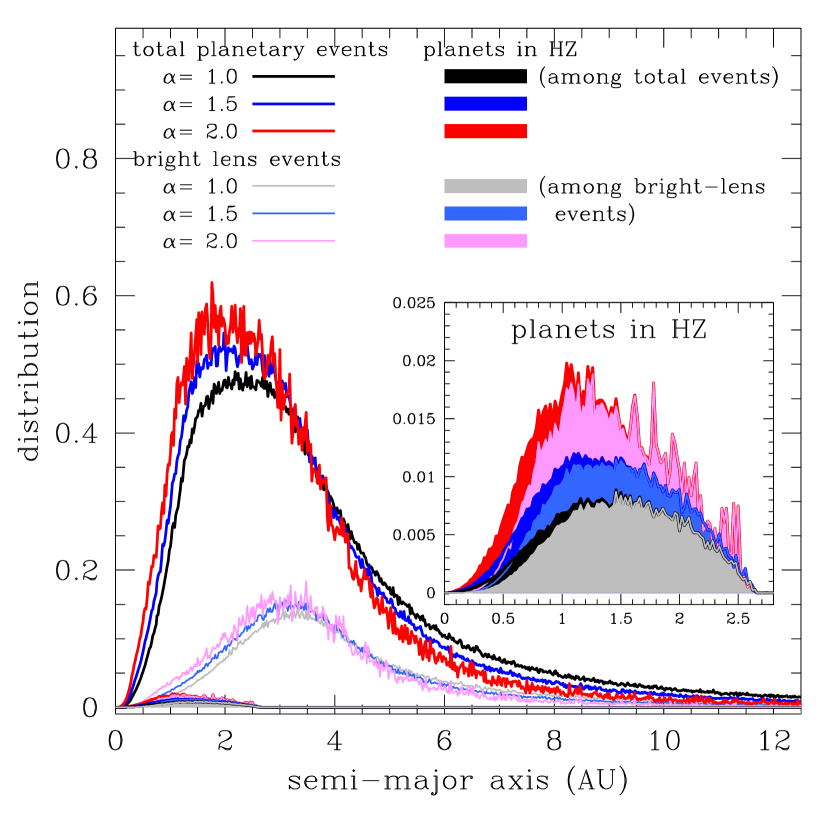
Figure 3.— The distributions of the semi-major axes of Earth-mass planets to be detected in future lensing surveys. The intrinsic semi-major axes of planets are assumed to be distributed by a power-law of the form $dN_{\rm p}/da\propto a^{-\alpha}$. The thick curves with black (for $\alpha=1.0$), blue ($\alpha=1.5$), and red ($\alpha=1.0$) colors represent the distributions of all planets, while the curves with grey ($\alpha=1.0$), light-blue ($\alpha=1.5$), and pink ($\alpha=2.0$) colors are the distributions of planets involved with bright lenses. The curves shaded with the corresponding colors are the distributions of planets located in the habitable zone.

Table 1Fraction of Planets in the Habitable Zone

distribution	definition of the	planet fraction in the habitable zone
model	habitable zone	out of total events	out of bright-lens events
$dN_{\rm p}/da\propto a^{-1.0}$	conservative	0.16%	0.71%
-	less-conservative	0.62%	2.70%
$dN_{\rm p}/da\propto a^{-1.5}$	conservative	0.26%	1.15%
-	less-conservative	0.88%	3.80%
$dN_{\rm p}/da\propto a^{-2.0}$	conservative	0.42%	1.74%
-	less-conservative	1.29%	5.40%

Note. — The fraction of habitable-zone Earth-mass planets to be detected in future lensing surveys. We present two fractions. One is the fraction out of the total number of planets ($f_{\rm HZ}$) and the other is the fraction among the planets involved with bright-lens events for which the primary lenses can be identified as stars ($f_{\rm HZ,\star}$). For the definitions of the conservative and less-conservative ranges of the habitable zone, see § 3. The models in the first column indicate the assumed distributions of the intrinsic semi-major axis of planets.

4. Results and Discussion

In Table 1, we summarize the resulting fractions of events with planets located in the habitable zone determined from the simulation. In Figure 3, we also present the semi-major axis distributions of the Earth-mass planets to be detected by the future lensing survey. In the figure, the thick curves with black (for the power $\alpha=1.0$ of the intrinsic semi-major axis distribution), blue ($\alpha=1.5$), and red ($\alpha=2.0$) colors represent the distributions of all planets, while the curves with grey ($\alpha=1.0$), light-blue ($\alpha=1.5$), and pink ($\alpha=2.0$) colors are the distributions for planets involved with bright lenses. The curves shaded with the corresponding colors are the distributions of planets located in the habitable zone. Here we use the less-conservative range.

From the table and figure, we find the following trends.

1. Planets located in the habitable zone comprises a very minor fraction of all planets. We find that the fraction ranges $f_{\rm HZ}\sim 0.2\%$ – 1.3% depending on the model distributions of the intrinsic semi-major axes and the definitions of the habitable zone. Bennett & Rhie (2002) predicted that the total number of Earth-mass planets that can be detected from the proposed space-based mission is $\sim 200$ if every lens star has an Earth-mass planet at an optimal position of 2.5 AU. Even under this optimistic expectation, then, the number of planets in the habitable zone will be at most $\sim 3$, which is not adequate enough for the statistical analysis on the frequency of terrestrial planets in the habitable zone.

2. Planets are biased toward smaller semi-major axis with the increase of the power $\alpha$ of the intrinsic semi-major axis distribution (c.f. the curves drawn with black [$\alpha=1.0$], blue [$\alpha=1.5$], and red [$\alpha=2.0$] colors). However, the dependence of the resulting semi-major axis distributions of lensing planets on $\alpha$ is weak.

3. Planets of bright lenses are biased toward larger semi-major axis compared to the distribution of the total planets. This is because bright lenses tend to be heavier and thus have larger mean radius of the lensing zone, i.e. $r_{\rm E}$.

4. Most of habitable-zone planets are associated with bright lenses (c.f. the pairs of curves shaded with black-gray, blue-light blue, and red-pink colors). This is because the gap between the lensing zone and habitable zone becomes narrower with the increase of the lens brightness. If the sample is confined only to planets involved with bright lens events, as a result, the fraction of habitable-zone planets increases into $f_{\rm HZ,\star}\sim 0.7\%$ – 5.4%.

Then, why is the microlensing sensitivity to Earth-mass planets located in the habitable zone so low? First of all, the projected star-planet separation at which the planet detection sensitivity becomes maximum is in most cases substantially larger than the median value of the habitable zone. This can be seen in Figure 2 where the ranges of the lensing zone and habitable zone are plotted as a function of the lens mass. Roughly, the median radius of the habitable zone is linearly proportional to the lens mass, while the mean value of the lensing zone is proportional to the square root of the mass. We find that the ratio of the median radius of the habitable zone to the mean radius of the lensing zone is roughly expressed as

$${d_{\rm HZ}\over r_{\rm E}}\sim 0.2\left({m\over 0.5\ M_{\odot}}\right)^{1/2}.$$ (11)

As a result, the two zones overlap only for stars more massive than the sun (Di Stefano, 1999). In addition, the habitable zone is defined by the intrinsic separation, while the lensing zone is defined by the projected separation. Considering the projection effect, then, the gap between the lensing zone and habitable zone further increases.

5. Conclusion

We investigated the microlensing sensitivity of future lensing surveys to Earth-mass planets located in the habitable zone by conducting detailed simulation of Galactic microlensing events. From the investigation, we found that the planets located in the habitable zone would comprise a very minor fraction and thus statistical analysis on the frequency of terrestrial planets in the habitable zone based on the sample would be very difficult. We find the main reason for the low sensitivity is that the projected star-planet separation at which the microlensing planet detection efficiency becomes maximum is in most cases substantially larger than the median value of the habitable zone.

References

- Allen (2000) Allen, C. W. 2000, Astrophysical Quantities, eds. A. N. Cox (The Athlon Press, London)
- An (2005) An, J. H. 2005, MNRAS, 356, 1409
- Angel (1994) Angel, J. R. P. 1994, Nature, 368, 203
- Baltz & Gondolo (2001) Baltz, E. A., & Gondolo, P. 2001, ApJ, 559, 41
- Bennett & Rhie (2002) Bennett, D. P., & Rhie, S. H. 2002, ApJ, 574, 985
- Bond et al. (2004) Bond, I. A., et al. 2004, ApJ, 606, L155
- Bozza (2000) Bozza, V. 2000, A&A, 355, 423
- Chung et al. (2005) Chung, S.-J., et al. 2005, ApJ, 630, 535
- Covone et al. (2000) Covone, G., de Ritis, R., Dominik, M., & Marino, A. A. 2000, A&A, 357, 810
- Di Stefano (1999) Di Stefano, R. 1999, ApJ, 512, 558
- Dwek et al. (1995) Dwek, E., et al. 1995, AJ, 445, 716
- Gould (2000) Gould, A. 2000, ApJ, 539, 928
- Gould, Gaudi, & Han (2004) Gould, A., Gaudi, B. S., & Han, C. 2004, ApJ, submitted (astro-ph/0405217)
- Gould, Ford, & Fischer (2003) Gould, A., Ford, E. B., & Fischer, D. A. 2003, ApJ, 591, L155
- Gould & Loeb (1992) Gould, A., & Loeb, A. 1992, ApJ, 396, 104
- Gould, Pepper, & DePoy (2003) Gould A., Pepper, J., & DePoy, D. L. 2003, ApJ, 594, 533
- Han (2005) Han, C. 2005, ApJ, 633, 414
- Han (2006) Han, C. 2006, ApJ, 638, 000
- Han & Gould (1995) Han, C., & Gould, A. 1995, ApJ, 447, 53
- Han & Gould (2003) Han, C., & Gould, A. 2003, ApJ, 592, 172
- Han et al. (2005) Han, C., Gaudi, B. S., An, J. H., & Gould, A. 2005, ApJ, 618, 962
- Hayashi (1995) Hayashi, S. S. 1995, Ap&SS, 224, 479
- Holtzman et al. (1998) Holtzman, J. A., Watson, A. M., Baum, W. A., Grillmair, C. J., Groth, E. J., Light, R. M., Lynds, R., & O’Neil, E. J. 1998, AJ, 115, 1946
- Kuchner (2004) Kuchner, M. J. 2004, ApJ, 612, 1147
- Lopez, Schneider & Danchi (2005) Lopez, B., Schneider, J., & Danchi, W. C. 2005, ApJ, 627, 974
- Marcy & Butler (1996) Marcy, G. W., & Butler, R. P. 1996, ApJ, 464, L147
- Mao & Paczyński (1991) Mao, S., & Paczyński, B. 1991, ApJ, 374, L37
- Mayor & Queloz (1995) Mayor, M., & Queloz, D. 1995, Nature, 378, 355
- Perryman (2000) Perryman, M. A. C. 2000, Rep. Prog. Phys., 63, 1209
- Perryman (2005) Perryman, M. A. C., et al. 2005, ESA-ESO Working Groups Report No. 1 (astro-ph/0506163)
- Sozzetti (2005) Sozzetti, A. 2005, PASP, 117, 1021
- Sozzetti et al. (2002) Sozzetti, A., Casertano, S., Brown, R. A., & Lattanzi, M. G., 2002, PASP, 114, 1173
- Stahl & Sandler (1995) Stahl, S. M., & Sandler, D. G. 1995, ApJ, 454, L153
- Struve (1952) Struve, O. 1952, Observatory, 72, 199
- Tabachnik & Tremaine (2002) Tabachnik, S., & Tremaine, S. 2002, MNRAS, 335, 151
- Udalski et al. (2005) Udalski, A., et al. 2005, ApJ, 628, L109
- Wolszczan & Frail (1992) Wolczan, A., & Frail, D. A. 1992, Nature, 355, 145
- Zoccali et al. (2000) Zoccali, M. S., Cassisi, S., Frogel, J. A., Gould, A., Ortolani, S., Renzini, A., Rich, M. A., & Stephens. A. 2000, ApJ, 530, 418