Spectra of the spreading layers on the neutron star surface and constraints on the neutron star equation of state

Abstract

Spectra of the spreading layers on the neutron star surface are calculated on the basis of the Inogamov-Sunyaev model taking into account general relativity correction to the surface gravity and considering various chemical composition of the accreting matter. Local (at a given latitude) spectra are similar to the X-ray burst spectra and are described by a diluted black body. Total spreading layer spectra are integrated accounting for the light bending, gravitational redshift, and the relativistic Doppler effect and aberration. They depend slightly on the inclination angle and on the luminosity. These spectra also can be fitted by a diluted black body with the color temperature depending mainly on a neutron star compactness. Owing to the fact that the flux from the spreading layer is close to the critical Eddington, we can put constraints on a neutron star radius without the need to know precisely the emitting region area or the distance to the source. The boundary layer spectra observed in the luminous low-mass X-ray binaries, and described by a black body of color temperature $T_{\rm c}=2.4\pm 0.1$ keV, restrict the neutron star radii to $R=14.8\pm 1.5$ km (for a 1.4-${\rm M}_{\odot}$ star and solar composition of the accreting matter), which corresponds to the hard equation of state.

1 Introduction

Matter accreting on to a weakly magnetized neutron star (NS) in low mass X-ray binaries (LMXRBs) can form an accretion disc which extend down to the NS surface. A boundary layer (BL) is formed between the accretion disc and the NS surface, where a rapidly rotating matter of the disc is decelerated down to the NS angular velocity. The amount of the energy, which is generated during this process, is comparable with the energy generated in the accretion disc (Sunyaev & Shakura, 1986; Sibgatullin & Sunyaev, 1998).

There is no generally accepted theory of the BL. Two different approaches to the BL description are considered. First of them, which we will call a ‘classical model’, considers the BL between a central star (a white dwarf or a NS) as a part of the accretion disc (Pringle, 1977; Pringle & Savonije, 1979; Tylenda, 1981; Shakura & Sunyaev, 1988; Bisnovatyi-Kogan, 1994; Popham & Narayan, 1995; Popham & Sunyaev, 2001). In this model the component of velocity normal to the accretion disc plane is zero. The half-thickness of the BL is determined by the same relation, as for the accretion disc:

$$H_{\rm BL}\sim\frac{c_{\rm s}}{v_{\rm K}}R,$$ (1)

where $c_{\rm s}$ is a sound speed in the BL and $v_{\rm K}$ is the Keplerian velocity close to the NS surface of radius $R$. The radial extension of the BL is determined by the relation (Pringle, 1977)

$$h_{\rm BL}\sim\frac{c^{2}_{\rm s}}{v^{2}_{\rm K}}R\sim H_{\rm BL}\frac{H_{\rm BL}}{R}.$$ (2)

In this classical model the accreting matter in the BL is decelerated in the accretion disc plane, along radial coordinate only, due to the viscosity operating within the differentially rotating BL, similarly to the accretion disc. From the observational point of view, the classical BL is a bright equatorial belt close to the NS surface. The effective temperature of the BL is higher than the maximum accretion disc effective temperature, because the BL is smaller than the accretion disc, while their luminosities are comparable.

Another approach was suggested by Inogamov & Sunyaev (1999, hereafter IS99). The BL is considered as a spreading layer (SL) on the NS surface. The accreting matter diffusing along the radial direction in the accretion disc and reaching the neutron star surface gains the velocity component normal to the accretion disc plane due to the ram pressure from the accretion disc. Then the matter spirals along the NS surface towards the poles. Rotating at the NS surface, the matter is decelerated due to a turbulent friction between the rapidly rotating matter and a slowly rotating NS surface. The kinetic energy of the accreting gas is mostly deposited in two bright belts at some latitude above and below the NS equator. The width and the latitude of the belts depend on the mass accretion rate. The larger the accretion rate, the wider the belts are and the closer they are to the NS poles. At the accretion rate close to the Eddington limit ($L_{\rm BL}\sim L_{\rm Edd}$) the bright belts expand all over the NS surface.

The observational difference between two BL models is not significant. At low accretion rates ($L_{\rm BL}\sim 0.01L_{\rm Edd}$) the latitude of bright belts of the SL is small ($\sim$ few degrees) and the vertical extension of the SL is comparable to the classical BL thickness. At high accretion rates ($L_{\rm BL}\sim L_{\rm Edd}$) the classical BL thickness is comparable to the NS radius (see Popham & Sunyaev, 2001). Therefore, the effective temperatures of these BL models are of the same order.

In the approach by IS99, the NS radius is assumed to be larger that $3R_{\rm S}$ (where $R_{\rm S}=2GM/c^{2}$ is the Schwarzschild radius of a NS of mass $M$), but the accretion disc structure is not significantly changed up to the NS surface, and the radial velocity is always subsonic. If the radial velocity of accreting gas is supersonic at the surface (see e.g. Popham & Narayan 1992, for a possibility of the supersonic radial velocity in classical BL, and Kluźniak & Wilson 1991, for the “gap accretion” when the NS is within the innermost stable circular orbit), some fraction of the kinetic energy (associated with a small radial velocity component) should be dissipated in an oblique shock, but most of it still remains stored in the kinetic energy of the gas rotating at the surface to be dissipated later in the SL. The gap accretion model of Kluźniak & Wilson (1991) is rather similar to the SL, but they did not consider the fate of the accreting material and its spread over the surface. At very low accretion rate, both models should produce hard Comptonization spectra extending to $\sim 100$ keV.

The aim of this work is the calculation of the radiation spectra of the SLs and their comparison to the observed X-ray spectra of the BLs in the luminous LMXRBs.

2 Spreading layer model

The theory of the SL was developed by IS99 under the assumption of Newtonian gravity. They considered accretion of the pure hydrogen plasma. Here we repeat the IS99 theory for plasmas of arbitrary chemical composition taking into account general relativity (GR) corrections using the pseudo-Newtonian potential. These corrections may be important, because the maximum effective temperature of the SL, which should be smaller than the local Eddington effective temperature $T_{\rm Edd}$, depends on the opacity and the gravity. The critical temperature is determined by the balance between the surface gravity and the radiative acceleration:

$$\frac{GM}{R^{2}\sqrt{1-R_{\rm S}/R}}=\frac{\sigma_{\rm SB}T_{\rm Edd}^{4}}{c}\sigma_{\rm e},$$ (3)

where $\sigma_{\rm e}=0.2(1+X)$ cm² g^-1 is the electron scattering opacity, $X$ is the hydrogen mass fraction, and $\sigma_{\rm SB}$ is the Stefan-Boltzmann constant. It is clear, that solar (or larger) helium abundance together with the GR correction will lead to higher $T_{\rm Edd}$, and, therefore, to a higher maximum effective temperature of the SL. This could have important consequences for the determination of the neutron star parameters from observations.

We use the pseudo-Newtonian potential in the form:

$$\Psi(r)=-c^{2}\left(1-\sqrt{1-R_{\rm S}/r}\right).$$ (4)

This potential gives the correct GR surface gravity

$$g_{\rm 0}(R)=\frac{GM}{R^{2}\sqrt{1-R_{\rm S}/R}},$$ (5)

but gives the Keplerian velocity at the NS surface

$$v^{2}_{\rm K}(R)=\frac{GM}{R\sqrt{1-R_{\rm S}/R}},$$ (6)

which is smaller than the correct GR value.

2.1 Main equations

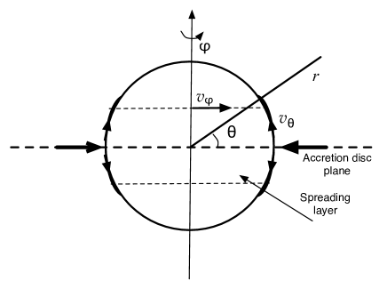
Figure 1: Geometry of the problem.

Below we rewrite the IS99 equations for the SL for the pseudo-Newtonian potential (4) and considering arbitrary abundances. We consider the dynamics of the SL on the NS surface (see Fig. 1). The full hydrodynamic equations, which describe this process are as follows (see for example Mihalas, 1978). The continuity equation is

$$\frac{\partial\rho}{\partial t}+{\bf\nabla\cdot}(\rho\mn@boldsymbol{v})=0,$$ (7)

where $\rho$ is the plasma density, $\mn@boldsymbol{v}$ is the vector of the gas velocity in the SL with components $v_{\varphi}$, $v_{\theta}$ and $v_{r}$, which are velocities of the SL along longitude, latitude and radius correspondingly. Conservation of momentum for each gas element is described by the vector Euler equation

$$\rho\frac{\partial\mn@boldsymbol{v}}{\partial t}+\rho\mn@boldsymbol{v}\cdot\nabla\mn@boldsymbol{v}=-\nabla P+\mn@boldsymbol{f},$$ (8)

where $P=P_{\rm rad}+P_{\rm g}$ is the total pressure which is a sum of the radiation and gas pressures, and $\mn@boldsymbol{f}$ is a force density. The energy equation for the gas in the SL is

$$\frac{\partial}{\partial t}\left(\frac{1}{2}\rho v^{2}+\varepsilon\right)+\nabla\cdot\left[\left(\frac{1}{2}\rho v^{2}+\varepsilon+P\right){\mn@boldsymbol{v}}\right]=$$ (9)

$$\mn@boldsymbol{f}\cdot\mn@boldsymbol{v}-\nabla\cdot\mn@boldsymbol{q}+Q^{+}.$$

Here $\varepsilon=\varepsilon_{\rm rad}+\varepsilon_{\rm g}$ is the total density of internal energy, where $\varepsilon_{\rm rad}=aT^{4}$ is the radiation energy density and $\varepsilon_{\rm g}=(3/2)P_{\rm g}$ is the density of the internal gas energy. The first term on the right hand side is the power produces by the force density, the second is the energy, which is lost by radiation ($\mn@boldsymbol{q}$ is a vector of the radiation flux), and the third is the heat, which is generated within a unit volume of the SL.

Following IS99 we consider the steady state SL model in the spherical coordinate system $(r,\theta,\varphi)$, where $\theta$ is the latitude and $\varphi$ is the azimuthal angle (see Fig. 1). We also assume that the SL has a small thickness (in comparison with the NS radius $R$, therefore the radial coordinate $r=R$), the radial velocity component is zero $v_{r}=0$, and it is axially symmetric (therefore, all of the derivatives $\partial/\partial\varphi$ equal to zero). In this case equations (7)–(9) take the following form. The continuity equation is

$$\frac{1}{R\cos\theta}\frac{\partial}{\partial\theta}(\cos\theta\ \rho v_{\theta})=0,$$ (10)

the three components of the Euler equation are

$$-\rho\left(\frac{v_{\theta}^{2}+v_{\varphi}^{2}}{R}\right)=-\frac{\partial P}{\partial r}+f_{r},$$ (11)

$$\rho\frac{v_{\theta}}{R}\frac{\partial v_{\theta}}{\partial\theta}+\rho\frac{v_{\varphi}^{2}}{R}\tan\theta=-\frac{1}{R}\frac{\partial P}{\partial\theta}+f_{\theta},$$ (12)

$$\rho\frac{v_{\theta}}{R}\frac{\partial v_{\varphi}}{\partial\theta}-\rho\frac{v_{\varphi}v_{\theta}}{R}\tan\theta=f_{\varphi},$$ (13)

and the energy equation is

$$\frac{1}{R\cos\theta}\frac{\partial}{\partial\theta}\left[\cos\theta\ v_{\theta}\left(\frac{1}{2}\rho v_{0}^{2}+\varepsilon+P\right)\right]=$$ (14)

$$f_{\theta}v_{\theta}+f_{\varphi}v_{\varphi}-\frac{\partial q}{\partial r}+Q^{+},$$

where

$$v_{0}^{2}=v_{\varphi}^{2}+v_{\theta}^{2}.$$ (15)

Here the radiation flux has only one (radial) non-zero component and its divergence is computed in the plane-parallel approximation which is a consequence of our assumption of small height of the SL. A small azimuthal component of the radiation flux arises due to the aberration, which we neglect here.

It is clear that equation (11) can be solved independently on equations (12)–(13) and we can consider some averaging over the layer’s height. Therefore, we arrive at a one-dimensional problem. In this case instead of equations (10)–(14) we obtain

$$\frac{1}{R\cos\theta}\frac{\partial}{\partial\theta}\left(\cos\theta\int\rho v_{\theta}{\rm d}r\right)=0,$$ (16)

$$\int\rho v_{\theta}\frac{\partial v_{\theta}}{\partial\theta}{\rm d}r+\tan\theta\int\rho v_{\varphi}^{2}{\rm d}r=-\frac{\partial}{\partial\theta}\int P{\rm d}r+R\int f_{\theta}{\rm d}r,$$ (17)

$$\int\rho v_{\theta}\frac{\partial v_{\varphi}}{\partial\theta}{\rm d}r-\tan\theta\int\rho v_{\varphi}v_{\theta}{\rm d}r=R\int f_{\varphi}{\rm d}r,$$ (18)

$$\frac{1}{R\cos\theta}\frac{\partial}{\partial\theta}\left[\cos\theta\int v_{\theta}\left(\frac{1}{2}\rho v_{0}^{2}+\varepsilon+P\right){\rm d}r\right]=$$ (19)

$$\int f_{\theta}v_{\theta}{\rm d}r+\int f_{\varphi}v_{\varphi}{\rm d}r-q+\int Q^{+}{\rm d}r.$$

Here the integration over radius is from $R$ to $R+h_{\rm S}$, where $h_{\rm S}$ is the local SL thickness. We define the corresponding force densities in the next section.

2.2 Vertical averaging

The one-dimensional equations for the SL structure are derived using the averaging along the height at a given latitude. It means that we have to calculate all the integrals in equations (16)–(19) for some model of the SL vertical structure. The simplest way is just to consider the variables averaged over the height.

IS99 used a more complicated model of averaging. They constructed a simple model of the SL using assumptions that velocities $v_{\theta}$, $v_{\varphi}$ and the radiation flux do not depend on the height $q(r)=\mbox{const}=\sigma_{\rm SB}T_{\rm eff}^{4}$. The latter suggestion means that all of the thermal energy in the SL is generated at the bottom. This model is described by the hydrostatic equilibrium equation (11) taken in the form

$$\frac{{\rm d}P}{{\rm d}m}=g_{\rm eff}\equiv g_{0}-\frac{v_{\varphi}^{2}+v_{\theta}^{2}}{R},$$ (20)

and the radiation transfer equation in the diffusion approximation

$$\frac{{\rm d}\varepsilon_{\rm rad}}{{\rm d}m}=\frac{3q}{c}\sigma_{\rm e}.$$ (21)

Here and below we use a new independent variable: a column mass $m$ and a new geometrical coordinate $z$, which are defined as

$${\rm d}m=\rho{\rm d}z=-\rho{\rm d}r.$$

Coordinate $z$ has an opposite direction relative to $r$ and $z$=0 at $r=R+h_{\rm S}$. We also defined the $r$ component of the force density

$$f_{r}=-g_{0}\rho.$$

Equations (20)–(21) have to be supplemented by the equation of state

$$P=\frac{\rho kT}{\mu m_{\rm p}}+\frac{\varepsilon_{\rm rad}}{3},$$ (22)

where $\mu=4/(3+5X)$ is the mean molecular weight and $m_{\rm p}$ is the proton mass.

Equations (20)–(22) can be solved with the simple boundary conditions $P(m=0)=0$, $T(m=0)=0$:

$$P=g_{\rm eff}m,$$ (23)

$$\varepsilon_{\rm rad}=\frac{3q}{c}m\sigma_{\rm e},$$ (24)

$$\rho=\mu m_{\rm p}\frac{g_{\rm cor}}{k}\left(\frac{ac}{3q\sigma_{\rm e}}m^{3}\right)^{1/4},$$ (25)

$$T=\left(\frac{3q}{ac}m\sigma_{\rm e}\right)^{1/4}=T_{\rm eff}\left(\frac{3}{4}\tau_{\rm e}\right)^{1/4},$$ (26)

where $\tau_{\rm e}=m\sigma_{\rm e}$ is the electron scattering optical depth of the layer, and

$$g_{\rm cor}\equiv g_{\rm eff}-g_{\rm rad}=g_{\rm eff}-\frac{q}{c}\sigma_{\rm e}.$$ (27)

The column density $m$ is related to the geometrical depth $z$

$$m=\frac{(\mu m_{\rm p}g_{\rm cor})^{4}}{4^{4}\sigma_{\rm e}k^{4}}\frac{ac}{3q}z^{4},$$ (28)

which gives the following dependence of temperature on height

$$T=\frac{\mu m_{\rm p}g_{\rm cor}}{4k}z.$$ (29)

Following IS99, we consider the values of temperature and density at the bottom of the SL $T_{\rm S}$ and $\rho_{\rm S}$ as parameters. In this case the local SL thickness $h_{\rm S}$ is:

$$h_{\rm S}=\frac{4kT_{\rm S}}{\mu m_{\rm p}g_{\rm cor}}.$$ (30)

We can also calculate all of the integrals in equations (16)–(19): the total surface density

$$\int_{0}^{h_{\rm S}}\rho{\rm d}z=m(z=h_{\rm S})=\Sigma_{\rm S},$$ (31)

the pressure surface density

$$\int^{h_{\rm S}}_{0}P{\rm d}z=\frac{1}{5}g_{\rm eff}h_{\rm S}\Sigma_{\rm S}=\frac{4}{5}\frac{g_{\rm eff}}{\mu m_{\rm p}g_{\rm cor}}\Sigma_{\rm S}kT_{\rm S},$$ (32)

the surface density of the internal energy

$$E_{\rm int}=\int^{h_{\rm S}}_{0}\left(\varepsilon_{\rm rad}+\frac{3}{2}P_{\rm g}\right){\rm d}z=\frac{3}{2}\left(g_{\rm eff}+g_{\rm rad}\right)\frac{\Sigma_{\rm S}h_{\rm S}}{5},$$ (33)

the local flux

$$q=\sigma_{\rm SB}T_{\rm eff}^{4}=\frac{ac}{3\sigma_{\rm e}}\frac{T_{\rm S}^{4}}{\Sigma_{\rm S}},$$ (34)

and the enthalpy flux

$$H=E_{\rm int}+\int^{h_{\rm S}}_{0}P{\rm d}z=\left(\frac{5}{2}g_{\rm eff}+\frac{3}{2}g_{\rm rad}\right)\frac{\Sigma_{\rm S}h_{\rm S}}{5}.$$ (35)

If we take $X=1$, all these relations will be the same, as derived by IS99 with one exception: there is no potential energy of the SL in our energy equation. Thus our expression for $H$ contains a factor $5/2$ instead of $7/2$ as in IS99. Below we will show that this produces only a small quantitative differences between our and IS99 models.

In the IS99 model there are two forces, which give contribution to the force density in equations (16)–(19). These are the gravity force, which has only the radial component (see above) and the force arising due to the friction between the NS surface and the SL. This force is directed along the NS surface and is expressed in the IS99 model through stress $\tau$ and its azimuthal and meridional components $\tau_{\varphi}$ and $\tau_{\theta}$. IS99 have parameterized it in the form:

$$\tau_{\varphi} = -\int_{0}^{h_{\rm S}}f_{\varphi}{\rm d}z=\alpha_{\rm b}\rho_{\rm S}v_{\varphi}v_{0},$$ (36)

$$\tau_{\theta} = -\int_{0}^{h_{\rm S}}f_{\theta}{\rm d}z=\alpha_{\rm b}\rho_{\rm S}v_{\theta}v_{0},$$

where $\alpha_{\rm b}=v_{*}^{2}/v_{0}^{2}$ is the parameter of the stress parametrization, $v_{*}$ is the velocity of turbulent pulsations. We should note that $\alpha_{\rm b}$ is not the same $\alpha$ that is used in the accretion disc theory. In accretion discs, $\alpha$ (in the first approximation) is the square of the ratio of the turbulent velocity to the sound speed $\alpha=v_{*}^{2}/c_{\rm s}^{2}$ and can be quite high, up to 0.1–1. In the SL, the plasma velocity $v_{0}$ is close to the Keplerian velocity at the NS surface and is orders of magnitude larger than the sound speed. The velocity of turbulent pulsation is also limited by the radiation viscosity at the SL bottom. IS99 carefully investigated this matter and estimated $\alpha_{\rm b}\sim 10^{-3}$. We used this value in most of the paper.

IS99 have ignored the mechanical work between the SL and the NS (which accelerates the stellar rotation). In our work we use the same approximation. A fraction of the kinetic energy of the accreting gas that goes to increase the rotational energy of the NS is approximately $2\Omega_{\rm*}/\Omega_{\rm K}$, where $\Omega_{\rm*}$ is the NS angular velocity and $\Omega_{\rm K}$ is the Keplerian angular velocity at the NS surface. As we consider a non-rotating NS and the characteristic time to increase its angular velocity is orders of magnitude larger than the characteristic time of the SL $t=R/v_{\theta}=10\ \mbox{km}/10^{3}\ \mbox{km s}^{-1}=0.01$ s, ignoring the mechanical work on the NS is a reasonable approximation. In this approximation, therefore, all the work due to friction between the SL and the NS transforms to heat:

$$\int_{0}^{h_{\rm S}}Q^{+}{\rm d}z=-(\tau_{\varphi}v_{\varphi}+\tau_{\theta}v_{\theta})=-\tau v_{0}.$$ (37)

2.3 One-dimensional model of the spreading layer

Using relations (30)–(37) we can rewrite equations, which describe the one-dimensional SL structure. The continuity equation can be rewritten via the accretion rate as

$$\dot{M}=4\pi R\ \cos\theta\ v_{\theta}\Sigma_{\rm S},$$ (38)

Therefore, the product $\cos\theta\ v_{\theta}\Sigma_{\rm S}=const$. The Euler equations are

$$\cos\theta\ v_{\theta}\Sigma_{\rm S}v_{\theta}^{\prime}+\frac{4}{5}\cos\theta\ \left(\frac{g_{\rm eff}}{g_{\rm cor}}\frac{kT_{\rm S}}{\mu m_{\rm p}}\Sigma_{\rm S}\right)^{\prime}=$$ (39)

$$-R\cos\theta\ \tau_{\theta}-\sin\theta\ \Sigma_{\rm S}v_{\varphi}^{2},$$

$$\Sigma_{\rm S}v_{\theta}(\cos\theta\ v_{\varphi})^{\prime}=-R\cos\theta\tau_{\varphi}.$$ (40)

Here the prime means the derivative over $\theta$. The second term in the left hand side of equation (39) is the lateral force gradient, and the terms in the right hand side are the components of the stress force and the centrifugal force. We see from equation (40) that the momentum along $\varphi$ coordinate is changed due to the friction with the NS surface only. The system of equations is closed by the energy equation

$$\Sigma_{\rm S}v_{\theta}\left(\frac{v_{0}^{2}}{2}+\frac{2}{5}\frac{kT_{\rm S}}{\mu m_{\rm p}}\frac{5g_{\rm eff}+3g_{\rm rad}}{g_{\rm cor}}\right)^{\prime}=-Rq.$$ (41)

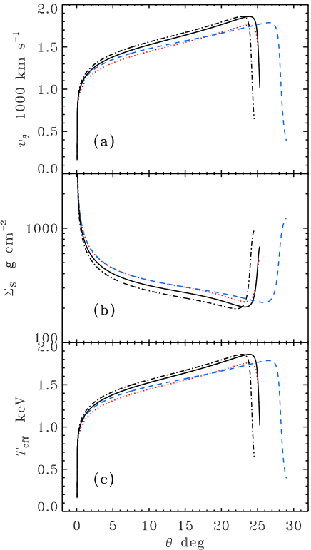
Figure 2: The distributions of (a) $v_{\theta}$, (b) the surface density $\Sigma_{\rm S}$ and (c) the effective temperature $T_{\rm eff}$ along latitude $\theta$ for four models. Solid and dashed curves are for our model corrected for the GR using pseudo-Newtonian potential and $X=0.7$ and $X=1$, respectively. The dotted curves is our model for the Newtonian gravity and $X=0.7$, while the dot-dashed curves are for the IS99 model corrected to GR and $X=0.7$. In all cases $M=1.4{\rm M}_{\odot}$ and $R$ = 12 km. The accretion rate of all models is the same, corresponding to $0.2L_{\rm Edd}$ of the first model.

The system of equations (38)–(41) can be transformed to the three dimensionless equations for $v_{\varphi}(\theta)$, $v_{\theta}(\theta)$ and $T_{\rm S}(\theta)$ as was done by IS99. These equations are solved with the boundary conditions at the transition zone between the accretion disc and the SL: the initial latitude, where the SL starts, is close to the NS equator $\theta_{\rm 0}\sim$ 10^-2; the initial relative deviation $\delta$ of $v_{\varphi}$ from the Keplerian velocity $v_{\varphi}=v_{\rm K}(1-\delta)$; and the initial ratio of the kinetic energy of the SL along $\theta$ coordinate and it’s thermal energy $\Theta\equiv(\mu m_{\rm p}v^{2}_{\theta_{0}})/kT_{\rm S}$.

As was demonstrated by IS99, the solution of equations (38)–(41) depends very little on $\theta_{0}$ (if $\theta_{0}$ sufficiently small $<0.1$, see below) and $\delta$, but strongly depend on parameter $\Theta$. We choose the solutions which are closest to the critical solution (in this solution $v_{\theta}$ is equal to the sound speed at the maximum latitude of the spreading layer), but slightly subsonic. The necessary critical value of parameter $\Theta$ is found by the bisection method.

The distributions of $v_{\theta}$, the effective temperature $T_{\rm eff}$, and the surface density $\Sigma_{\rm S}$ along the latitude $\theta$ for four models with the same accretion rate, corresponding to first model luminosity are shown in Fig. 2. The first model (shown by the solid curves) is our model with the pseudo-Newtonian potential and solar hydrogen abundance $X=0.7$. The dashed curves are for our model with GR correction, but with pure hydrogen $X=1$; the dotted curves correspond to our model without GR corrections ($R_{\rm S}=0$ in the equations) with solar hydrogen abundance ($X=0.7$), while the dot-dashed curves are for the IS99 model with GR corrections and solar hydrogen abundance. It is clear that the solar abundance lead to a narrower spreading layer with a smaller surface density. A higher helium abundance as well as the the GR corrections lead to a higher effective temperature and a larger latitudinal velocity. Our model gives a slightly wider SL with slightly smaller latitudinal velocity but same effective temperature and surface density. Most calculations below were performed for our model with the GR correction and solar abundances. The surface density and the effective temperature distributions along the latitude for models with 0.1, 0.2, 0.4 and 0.8 of the Eddington luminosity are presented in Fig. 3. Variations of parameter $\alpha_{\rm b}$ lead to some changes in the SL structure. The SL column density is inversely proportional to $\alpha_{\rm b}$, while the resulting effective temperature decreases only by about 1 per cent with decreasing of $\alpha_{\rm b}$ by an order of magnitude.

Figure 3: The distributions of the surface density $\Sigma_{\rm S}$ and the effective temperature $T_{\rm eff}$ over the latitude $\theta$ for the SL models with different luminosities. Initial SL latitude is $\theta_{0}=10^{-2}$.

The lower boundary of the SL was taken very close to the equator, $\theta_{\rm 0}\approx 0.01-0.001$, in IS99. Formally, the accretion disc thickness is close to zero at the inner boundary, if we take the usual inner boundary condition for the component of the stress tensor $W_{r\varphi}(R_{\rm in})=0$. In the case of the accretion disc around a NS this condition is not correct, and the disc thickness at the NS surface is considerable. The luminous accretion disc half-thickness can be evaluated from the balance of the radiation force and $z$-component of gravity:

$$z_{0}=\frac{3\sigma_{\rm e}}{8\pi c}\dot{M}.$$ (42)

We calculated the SL models with the initial latitudes $\theta_{01}=\arcsin(z_{0}/R)$ and $\theta_{02}=\arcsin(0.5z_{0}/R)$. The surface density and the effective temperature distributions along the latitude for the second case are shown in Fig. 4 . The qualitative behavior of these distributions is close to the case of small $\theta_{0}$ with some shift along the latitude. The main difference is the maximum possible luminosity of the SL. At this luminosity the SL reaches the NS poles. For $\theta_{02}$, the maximum possible luminosity is about 0.4 $L_{\rm Edd}$, while for $\theta_{01}$ it is about 0.25 $L_{\rm Edd}$.

Figure 4: The distributions of the surface density $\Sigma_{\rm S}$ and the effective temperature $T_{\rm eff}$ along latitude $\theta$ for SL models with different luminosities. Initial SL latitude $\theta_{0}=\arcsin(0.5z_{0}/R)$.

2.4 Vertical structure of the spreading layer

The IS99 SL model was constructed under an assumption that the local layer velocity and the radiation flux along height is constant. It means that the SL is decelerated and energy is liberated in the infinitely thin layer at the NS surface. This is an approximation only and the velocity distribution should not be uniform and the energy should be generated at all heights. Therefore, we need a more detailed vertical model of the SL for calculating its radiation spectrum.

For evaluation of the viscosity parameter $\alpha_{\rm b}$, IS99 used classical theory of hydrodynamic BLs (Landau & Lifshitz, 1959) with the logarithmic velocity and the energy generation distribution along the height. In this case, both the energy generation rate and the velocity gradient are inversely proportional to the distance from the NS surface $z$

$$\frac{{\rm d}q}{{\rm d}z}\propto\frac{{\rm d}v}{{\rm d}z}\propto\frac{1}{z}.$$ (43)

It is clear that these dependencies cannot be correct in a SL. The SL has a finite thickness with a low density at the surface. However according to equation (43) some amount of energy has to be generated in the surface layers.

At present time, a theory of the radiation-dominated turbulent boundary layer does not exist. Thus we here can only make similar assumptions about the energy generation and velocity gradient along the height. We assume that these values are inversely proportional to the surface density measured from the NS surface:

$$\frac{{\rm d}q}{{\rm d}m}=-A~{}\frac{q_{\rm 0}}{\Sigma_{\rm S}-m},$$ (44)

$$\frac{{\rm d}v}{{\rm d}m}=-A~{}\frac{v_{0}}{\Sigma_{\rm S}-m},$$ (45)

where $A=2.5\alpha_{\rm b}^{1/2}$, $q_{\rm 0}$ and $v_{0}$ are the local radiation flux and the average layer velocity at a given latitude obtained from the one-dimensional model. Equations (44) and (45) are very close to the IS99 SL model assumptions (the layer is decelerated and the energy is generated at the bottom of the layer). Integration of these equations yields

$$q(m)=q_{\rm 0}\left[1+A~{}\ln\left(1-\frac{m}{\Sigma_{\rm S}}\right)\right],$$ (46)

$$v(m)=v_{0}\left[1+A~{}\ln\left(1-\frac{m}{\Sigma_{\rm S}}\right)\right].$$ (47)

These equations can be used up to some critical column density

$$m_{*}=\Sigma_{\rm S}\left(1-\exp[-A^{-1}]\right),$$ (48)

which is very close to the local surface density.

The hydrostatic equilibrium equation then reads

$$\frac{{\rm d}P_{\rm g}}{{\rm d}m}=g_{\rm 0}-\frac{v^{2}(m)}{R}-\frac{q(m)}{c}\sigma_{\rm e}$$ (49)

and the radiation transfer equation is

$$\frac{1}{3}\frac{{\rm d}\varepsilon}{{\rm d}m}=\frac{q(m)}{c}\sigma_{\rm e}.$$ (50)

The temperature and the gas pressure distributions along the height are:

$$T(m) = T_{\rm eff}~{}\left[\frac{3}{4}m\sigma_{\rm e}\ \left(1-A\left[1+\frac{\Sigma_{\rm S}-m}{m}\right.\right.\right.$$

$$\times \left.\left.\left.\ln\left(1-\frac{m}{\Sigma_{\rm S}}\right)\right]\right)+\frac{1}{2}\right]^{1/4}$$

$$P_{\rm g}(m) = g_{0}m-\frac{v^{2}_{0}}{R}m\left(1-2A+2A^{2}\right)$$

$$+ \frac{v^{2}_{0}}{R}A\left(\Sigma_{\rm S}-m\right)\ln\left(1-\frac{m}{\Sigma_{\rm S}}\right)$$

$$\times \left[A~{}\ln\left(1-\frac{m}{\Sigma_{\rm S}}\right)-2A+2\right]$$

$$- \frac{q_{0}\sigma_{\rm e}}{c}\left[m-A\left(m+\left(\Sigma_{\rm S}-m\right)\ln\left(1-\frac{m}{\Sigma_{\rm S}}\right)\right)\right].$$

These solutions are obtained using the boundary conditions at the surface $\varepsilon(m=0)=2q_{0}/c$ and $P_{\rm g}(m=0)=0$.

At the same time, there is a disagreement between this vertically explicit model and one-dimensional model, because the velocity and the flux vertical profiles are different. We suggest, that the model can be made self-consistent, if we find a new value of the surface density $\Sigma_{\rm S}^{\prime}$ at a given latitude, which conserves the mass flux

$$v_{0}\Sigma_{\rm S}=\int_{0}^{\Sigma_{\rm S}^{\prime}}v(m){\rm d}m=v_{0}(1-A)\Sigma_{\rm S}^{\prime}.$$ (53)

Therefore, the new value of the surface density $\Sigma_{\rm S}^{\prime}=\Sigma_{\rm S}/(1-A)$. For $\alpha_{\rm b}=10^{-3}$, this gives $\Sigma_{\rm S}^{\prime}=1.086\Sigma_{\rm S}$ and we take these values below for our calculations. There are similar disagreements for other integrals over the height in equations (16)–(19). For example:

$$v_{0}^{2}\Sigma_{\rm S}=\int_{0}^{\Sigma_{\rm S}^{\prime}}v^{2}(m){\rm d}m=v_{0}(1-2A+A^{2})\Sigma_{\rm S}^{\prime}.$$ (54)

In this case, we have to take a new value of the surface density $\Sigma_{\rm S}^{\prime}=\Sigma_{\rm S}/(1-2A+A^{2})$, which gives $\Sigma_{\rm S}^{\prime}=1.171\Sigma_{\rm S}$ if $\alpha_{\rm b}=10^{-3}$. Our vertically explicit models disagree with the one-dimensional ones by about 10 per cent. Fortunately, the emitted local spectra depend very little on the surface density of the SL.

3 Spectrum of the spreading layer

For calculation of the SL spectra we divide it into a number of rings over the latitude which have different effective temperatures $T_{\rm eff}$, matter velocities $v_{0}$ and surface densities $\Sigma_{\rm S}$. We then calculate the vertically explicit model for each ring, solve the radiative transfer equation and obtain the local SL spectrum. Then we integrate local spectra from the SL surface accounting for the general and special relativity effects.

3.1 Local spectra

To calculate a vertically explicit hydrodynamical model with the radiation transfer we use standard methods for stellar atmospheres modelling (Mihalas, 1978). Our models are obtained in the hydrostatic and the plane-parallel approximations. The effective temperatures of the considered SL models are rather high ($\sim$ 2 keV) and these models are similar to the atmospheres of bursting NSs, where Compton scattering have to be taken into account.

The vertically explicit local SL model is described by the following equations: the equation of hydrostatic equilibrium (49), the energy generation law (46), the velocity law (47), the RTE accounting for the Compton effect using the Kompaneets (1957) operator:

$$\frac{\partial^{2}(f_{\nu}J_{\nu})}{\partial\tau_{\nu}^{2}}=\frac{k_{\nu}}{k_{\nu}+\sigma_{\rm e}}\left(J_{\nu}-B_{\nu}\right)-\frac{\sigma_{\rm e}}{k_{\nu}+\sigma_{\rm e}}\frac{kT}{m_{\rm e}c^{2}}\times$$ (55)

$$x\frac{\partial}{\partial x}\left(x\frac{\partial J_{\nu}}{\partial x}-3J_{\nu}+\frac{T_{\rm eff}}{T}xJ_{\nu}\left[1+\frac{CJ_{\nu}}{x^{3}}\right]\right),$$

where $x=h\nu/kT_{\rm eff}$ is dimensionless frequency, $f_{\nu}(\tau_{\nu})\approx 1/3$ is the variable Eddington factor, $J_{\nu}$ is the mean intensity of radiation, $B_{\nu}$ is the black body (Planck) intensity, $k_{\nu}$ is the opacity due to the free-free and bound-free transitions, $\sigma_{\rm e}$ is the electron (Thomson) opacity, $T$ is the local electron temperature, $T_{\rm eff}$ is the effective temperature of SL at a given latitude, and $C=c^{2}h^{2}/2(kT_{\rm eff})^{3}$. The optical depth $\tau_{\nu}$ is defined as

$${\rm d}\tau_{\nu}=(k_{\nu}+\sigma_{\rm e}){\rm d}m.$$ (56)

These equations have to be completed by the energy balance equation

$$\int_{0}^{\infty}k_{\nu}\left(J_{\nu}-B_{\nu}\right){\rm d}\nu-\frac{1}{4\pi}\frac{{\rm d}q}{{\rm d}m}-\sigma_{\rm e}\frac{kT}{m_{\rm e}c^{2}}\times$$ (57)

$$\left[4\int_{0}^{\infty}J_{\nu}{\rm d}\nu-\frac{T_{\rm eff}}{T}\int_{0}^{\infty}xJ_{\nu}\left(1+\frac{CJ_{\nu}}{x^{3}}\right){\rm d}\nu\right]=0$$

and by the ideal gas law

$$P_{\rm g}=N_{\rm tot}kT,$$ (58)

where $N_{\rm tot}$ is the number density of all particles, as well as by the particle and charge conservation laws. We assume local thermodynamical equilibrium (LTE) in our calculations, so the number densities of all ionization and excitation states of all elements have been calculated using Boltzmann and Saha equations.

For solving these equations and computing the local SL model we used the Kurucz’s code ATLAS (Kurucz, 1970, 1993) modified for high temperature. All ionization states of the 15 most abundant elements are taken into consideration. The photoionization cross-sections from the ground states of all ions are calculated using phfit2 code (Verner et al., 1996). For details see Swartz et al. (2002) and Ibragimov et al. (2003). The code was also modified to account for Compton scattering.

The scheme of calculation is the following. First, the input parameters of the local SL model are defined from the total one-dimensional SL model (see Sect. 2.3): the effective temperature $T_{\rm eff}$, the surface gravity $g_{0}$, the surface density $\Sigma_{\rm S}$, and the local average layer velocity $v_{0}$. Then the analytical vertically explicit model (2.4–53) are calculated together with the new value of surface density $\Sigma_{\rm S}^{\prime}=\Sigma_{\rm S}/(1-A)$. The calculations are performed for the set of 98 column densities $m$, distributed logarithmically with equal steps from $m=10^{-5}$ g cm^-2 to $0.99m_{*}$. The gas pressure, which is found from equation (2.4), is not varied during the iterations.

For this starting model, all number densities and the opacities at all depth points and all the frequencies (we use 300 logarithmically equidistant frequency points) are calculated. The RTE (55) is solved by the Feautrier method (Mihalas, 1978; Zavlin & Shibanov, 1991; Pavlov et al., 1991; Grebenev & Sunyaev, 2002) iteratively, because it is non-linear. Between the iterations we calculate the variable Eddington factors $f_{\nu}$ and $h_{\nu}$, using the formal solution of the RTE for three angles. Usually 5–6 iterations are sufficient to achieve convergence.

We used the usual condition at the outer boundary

$$\frac{\partial(f_{\rm\nu}J_{\nu})}{\partial\tau_{\nu}}=h_{\nu}J_{\nu},$$ (59)

where $h_{\nu}$ is the surface variable Eddington factor, and the inner boundary condition

$$\frac{\partial J_{\nu}}{\partial\tau_{\nu}}=\frac{\partial B_{\nu}}{\partial\tau_{\nu}}.$$ (60)

The outer boundary condition is found from the lack of the incoming radiation at the SL surface, and the inner boundary condition is obtained from the diffusion approximation $J_{\nu}\approx B_{\nu}$ and $q_{\nu}\approx 4\pi/3\times\partial B_{\nu}/\partial\tau_{\nu}$. This condition is satisfied for any SL optical thickness, because the SL bottom is the NS surface. The boundary conditions along the frequency axis are

$$J_{\nu}=B_{\nu}$$ (61)

at the lower frequency boundary, $\nu=\nu_{\rm min}=10^{14}$ Hz ($h\nu_{\rm min}\approx$ 0.03 eV $\ll kT_{\rm eff}$) and

$$x\frac{\partial J_{\nu}}{\partial x}-3J_{\nu}+\frac{T_{\rm eff}}{T}xJ_{\nu}\left(1+\frac{CJ_{\nu}}{x^{3}}\right)=0$$ (62)

at the higher frequency boundary $\nu=\nu_{\rm max}=3\ 10^{19}$ Hz ($h\nu_{\rm max}\approx$ 100 keV $\gg kT_{\rm eff}$). Condition (61) means that at the lowest energies the true opacity dominates the scattering $k_{\nu}\gg\sigma_{\rm e}$, and therefore $J_{\nu}\approx B_{\nu}$. Condition (62) means that there is no photon flux along the frequency axis at the highest energy.

The solution of the RTE (55) should also satisfy the energy balance equation (57) and the surface flux condition

$$\int_{0}^{\infty}q_{\nu}(m=0){\rm d}\nu=\sigma_{\rm SB}T_{\rm eff}^{4}.$$ (63)

We calculated the relative flux error along the depth

$$\varepsilon_{q}(m)=1-\frac{q(m)}{\int_{0}^{\infty}q_{\nu}(m){\rm d}\nu},$$ (64)

where $q(m)$ is found from the energy generation law (46), and $q_{\nu}(m)$ is radiation flux at a given depth obtained from the first moment of the RTE

$$4\pi\frac{\partial(f_{\nu}J_{\nu})}{\partial\tau_{\nu}}=q_{\nu}.$$ (65)

Then the temperature corrections were evaluated using three different procedures. The first procedure is the integral $\Lambda$-iteration method based on the energy balance equation (57) which was modified to account for Compton scattering. It works well in the upper layers. The second one is the modified Avrett-Krook flux correction, which uses the relative flux error and is good in deep layers. And the third one is the surface correction, which is based on the emergent flux error. See Kurucz (1970) for the detailed description of the methods.

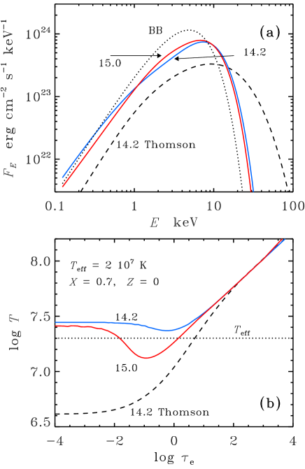
Figure 5: (a) The spectra of the bursting NS model atmospheres with the effective temperature $T_{\rm eff}$ = $2\ 10^{7}$ K, solar hydrogen/helium abundances without heavy elements and $\log~{}g$ = 14.2 and 15. The black body spectrum corresponding to the effective temperature is shown by the dotted curve. (b) The corresponding temperature structure as a function of the Thomson optical depth. The dashed curves show the spectrum and the temperature structure for one model computed not accounting for Compton scattering.

The iteration procedure is repeated until the relative flux error is smaller than 1 per cent, and the relative flux derivative error is smaller than 0.01 per cent. As a result we obtain the self-consistent local SL model together with the emergent spectrum of radiation.

Our method of calculation was checked on the atmosphere model of bursting NS. The equations which describe the bursting atmosphere are simpler, because there is no velocity field along the surface ($v_{0}=0$) and the integral flux is constant along depth (${\rm d}q/{\rm d}m=0$). We compared our model atmospheres with the most recent models of Madej, Joss & Różańska (2004). The radiation spectra and the temperature structure for some models with $T_{\rm eff}=2\ 10^{7}$ K, solar H/He abundances, and various surface gravities are shown in Fig. 5. These results are in a perfect agreement with the results of Madej et al. (2004). The emergent spectra and the temperature structure for the models with the solar abundance of heavy elements are shown in Fig. 6.

In the surface layers, local cooling is small because of the low density, and the temperature equals the Compton temperature of radiation which is slightly higher than the effective temperature. In dipper layers, at $\tau_{\rm e}\sim 0.1$, the cooling due to thermal emission (free-free and bound-free) becomes important (as thermal emissivity per gram is proportional to density) and the temperature decreases. At large optical depth the temperature rises again and follows the $\tau_{\rm e}^{1/4}$ relation, typical for a grey atmosphere. At higher surface gravity (at fixed $T_{\rm eff}$), the plasma density is higher, resulting in a more significant temperature dip. We see that heavy elements have rather minimal influence on the models close to the Eddington limit (lower $g$).

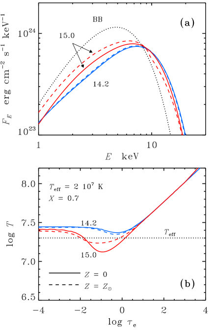
Figure 6: Dependence of the bursting NS model atmospheres on metal abundance. Dashed curves correspond to the solar abundance of metals and solid curves to the zero metal abundance. Examples are for solar H/He abundances, the same effective temperature $T_{\rm eff}$ = $2\ 10^{7}$ K and two values of $\log~{}g$ = 14.2 and 15. Black body spectrum corresponding to the effective temperature is shown by dotted curve.

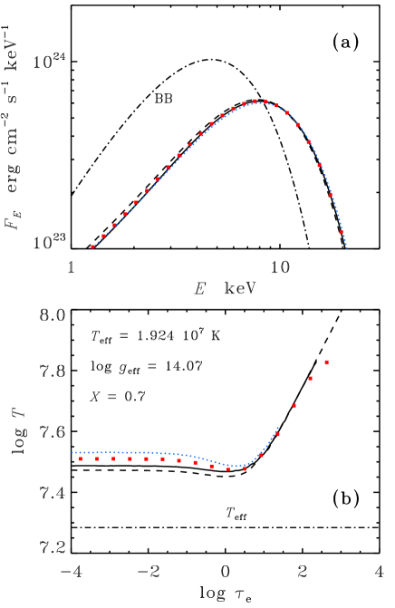
Figure 7: Comparison of the bursting NS model (dashed curves) and different local SL models for the same $T_{\rm eff}$ and effective gravity $\log~{}g$. Solid curves correspond to the local SL model (with the vertical structure model described in section  2.4) with surface density $\Sigma_{\rm S}=630\ \mbox{g cm}^{-2}$. The spectrum and the temperature structure of the local SL model with the constant velocity and flux derivatives are shown by squares. Dotted curves correspond to local SL model (Sect. 2.4) with $\Sigma_{\rm S}=63\ \mbox{g cm}^{-2}$.

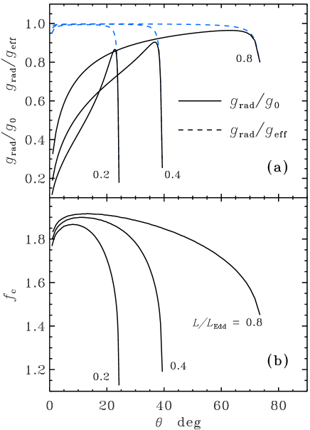
Figure 8: (a) Radiative and effective accelerations and (b) the hardness factor $f_{\rm c}$ (b) as functions of latitude for the SL models of different luminosities $L/L_{\rm Edd}$.

The comparison between the bursting NS models and different local SL models for the same $T_{\rm eff}$ and effective $\log g$ is shown in Fig. 7. For this SL model we use the vertical structure model, which is described in Section 2.4. We also investigated, whether the model for the vertical structure is important for the emergent spectra of local SL models. We also calculated the SL model with the constant velocity and flux derivatives:

$$\frac{{\rm d}v}{{\rm d}m}=-\frac{v_{0}}{\Sigma_{\rm S}}$$ (66)

and

$$\frac{{\rm d}q}{{\rm d}m}=-\frac{q_{0}}{\Sigma_{\rm S}}.$$ (67)

In this case the mass flux conservation requirement (53) leads to $\Sigma_{\rm S}^{\prime}=2\Sigma_{\rm S}$. The spectrum and the temperature structure of this model are shown in Fig. 7 by squares. The surface temperatures of the local SL models are higher than the bursting NS model surface temperature. The reason is the non-zero flux derivative in the energy conservation equation (57). This means that a part of the energy is released in the upper atmosphere and is heating it additionally. The smaller the surface density (i.e. the larger the flux derivative), the higher the surface temperature. But the differences in the temperature structure have very small influence on the emergent spectra. Therefore we conclude, that details of the vertical structure have negligible influence on the emergent spectrum for the optically thick models ($\Sigma_{\rm S}\geq 100\ \mbox{g cm}^{-2}$).

It is well known that the model spectra of bursting NS close to the Eddington limit are well described by a diluted Planck spectrum with the color temperature $T_{\rm c}=f_{\rm c}T_{\rm eff}$ with the hardness factor $f_{\rm c}$ varying in the interval 1.6–1.9 and the dilution factor $D=f_{\rm c}^{-4}$. Pavlov et al. (1991) have derived an analytical formula for the hardness factor, which successfully describes high luminosity ($L\approx L_{\rm Edd}$) burst spectra:

$$f_{\rm c}=\left(0.15\ \ln C_{1}+0.59\right)^{-4/5}C_{1}^{2/15}\ell^{3/20},$$ (68)

where $C_{1}=(3+5X)/(1-\ell)$ and $\ell=L/L_{\rm Edd}=g_{\rm rad}/g_{\rm eff}$. Equation (68) works well also for models with heavy elements.

The local spectra of the optically thick SL (with $L>0.2L_{\rm Edd}$) are very similar to the burst spectra with corresponding parameters (see Fig.  7). The local SL are very close to the Eddington limit

$$g_{\rm rad}=\frac{q_{0}}{c}\sigma_{\rm e}\approx g_{0}-\frac{v_{0}^{2}}{R}=g_{\rm eff}.$$ (69)

For example, the distributions of the ratios $g_{\rm rad}/g_{0}$ and $g_{\rm rad}/g_{\rm eff}$ along the latitude for SL models with three different luminosities are shown in Fig. 8a. Corresponding hardness factor distributions are shown in Fig. 8b. The comparison of the two local SL spectra (close to equator and at higher latitude) with the diluted Planck spectra and hardness factors given by equation (68) are shown in Fig. 9a. Closer to the equator, effective gravity is low as centrifugal force is large. The gas is levitating above the NS and $\ell$ is close to unity. The energy dissipation and the effective temperature are low. Thus, $f_{\rm c}$ is large and the spectrum is close to the diluted Planck. At higher latitude, the layer is decelerated, while the energy dissipation and $T_{\rm eff}$ grow. However, the effective gravity grows faster reducing $\ell$ and the color correction $f_{\rm c}$. The spectrum shows deviations from the diluted Planck spectrum at low energies. At high energies, the Wien part of both spectra can well be described by the diluted Planck.

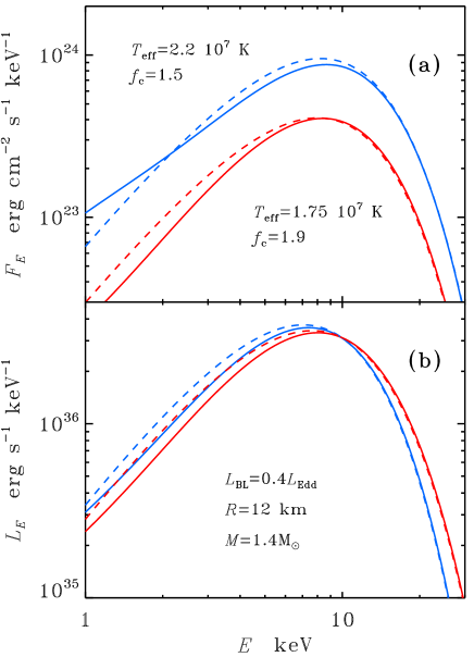
Figure 9: (a) Local SL model spectra with high and low effective temperatures (solid curves) compared to the diluted Planck spectra with $f_{\rm c}$ given by equation (68). (b) Integral spectra (isotropic luminosities) of the same SL model (solid curves) for different inclination angles $i=0\degr$ (softer spectrum) and $90\degr$ (harder spectrum) compared to the total spectra obtained by integration of the diluted Planck spectra (dashed curves).

3.2 Integral spectra

Now we can compute the integral total model spectrum of the SL, which is seen by a distant observer accounting for the relativistic effects such as gravitational redshift, light bending, relativistic Doppler effect and aberration. We take into account only half of the SL because another half is hidden by the accretion disc and divide the SL surface on 10 latitude rings and on 100 angles in azimuth. In a spherical coordinate system, where the accretion disc coincides with the $\theta=0\degr$ plane, the spectrum of the SL is (Poutanen & Gierliński, 2003)

$$F_{\rm E}=\frac{R^{2}}{D^{2}}\int\limits_{0}^{\theta_{\rm SL}}\int\limits_{0}^{2\pi}\eta^{3}\delta^{3}I(E^{\prime},\cos\alpha^{\prime},\theta)\cos\alpha^{\prime}\cos\theta\ {\rm d}\theta\ {\rm d}\varphi.$$ (70)

Here the observed and the emitted photon energies are connected by the relation $E=E^{\prime}\ \eta\ \delta$, where $\eta=\sqrt{1-R_{\rm S}/R}$, the Doppler factor $\delta=1/\gamma(1-\beta\cos\xi)$, $\beta=v_{\varphi}(\theta)/c$ (here we neglected low latitudinal velocity), the Lorentz factor $\gamma=1/\sqrt{1-\beta^{2}}$, and $\cos\xi=-\sin\alpha\ \sin i\ \sin\varphi/\sin\psi$. The light bending is accounted for by the relation (Beloborodov, 2002)

$$\cos\alpha=\frac{R_{\rm S}}{R}+\eta^{2}\cos\psi,$$ (71)

where $\cos\psi=\cos i\sin\theta+\sin i\cos\theta\cos\varphi$, and the relativistic aberration gives $\cos\alpha^{\prime}=\delta\cos\alpha$ (Poutanen & Gierliński, 2003). Here $i$ is the inclination angle of the NS polar axis to the line of sight, $D$ is the distance to the observer, and $\theta_{\rm SL}$ is the SL boundary. Only visible surface elements with $\cos\alpha>0$ give contribution to the total spectrum.

Figure 10: Specific intensities of the emerging radiation of the local SL model (here $\mu=\cos\alpha^{\prime}$) with the same parameters as in Fig. 7 computed exactly (solid curves) and using formula (72).

The emitted specific intensity $I(E^{\prime},\cos\alpha^{\prime},\theta)$ is taken from the computed local SL flux assuming angular dependence for the electron scattering atmosphere

$$I(E^{\prime},\cos\alpha^{\prime},\theta)=\frac{q_{\rm E^{\prime}}(\theta)}{\pi}(0.4215+0.86775\cos\alpha^{\prime}).$$ (72)

This formula gives a good approximation to the specific intensity of the emergent radiation (see Fig. 10).

Figure 11: Dependence of the SL integral spectra on the inclination angle $i$ to the line of sight (a) and on the luminosity (b).

The total spectra of the SL model for two inclination angles, $i=0{\degr}$ and $90{\degr}$, are shown in Fig. 9b. The spectra computed using the local diluted Planck spectra are shown also for comparison. The difference is very small in the high energy part ($E>10$ keV) and more significant at lower energies ($E<7$ keV).

Dependence of spectral shape on the inclination angle is not significant (see also Fig. 11a). Differences between the SL spectra, which are seen at different inclinations are comparable to the differences due to change in the SL luminosities (see Fig. 11b). It is interesting, that the total spectra can also be well described by the diluted Planck spectrum.

The color temperature depends slightly on the assumed turbulence parameter $\alpha_{\rm b}$. Decreasing $\alpha_{\rm b}$ by an order of magnitude increases $T_{\rm c}$ by 0.1 keV.

4 Comparison with observations

In LMXRBs a weakly magnetized NS is surrounded by the accretion disc which transforms to the boundary/SL close to the NS surface. At present, about 100 LMXRBs are known. They can be divided into two different classes. The Z-sources are very luminous ($L\sim 0.1-1L_{\rm Edd}$) and have relatively soft, two-component spectra. Both components are close to the black body with color temperatures of about 1 keV and 2–2.5 keV. The atoll sources are less luminous ($L\sim 0.01-0.05L_{\rm Edd}$) and are observed in two states, the high/soft and the low/hard. In the soft state, the radiation spectra are similar to those of the Z-sources, while in the hard state they are close to the spectra of the Galactic black hole sources in the hard states (e.g. Cyg X-1, see e.g. Poutanen, 1998; Barret et al., 2000). These hard spectra are well described by unsaturated Comptonization of soft photons in the hot ($kT\sim$ 30 – 100 keV) optically thin ($\tau_{\rm e}\sim$ 1) plasma.

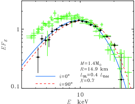
Figure 12: Comparison of the observed spectra of the BLs of LMXRBs obtained by the Fourier-frequency resolved spectroscopy and the model spectra of the SL at two inclination angles to the line of sight. Filled circles give the spectrum of GX 340+0 in the normal branch (see Fig. 12 in Gilfanov et al., 2003), open circles correspond to the spectra of five Z- and atoll sources (from Revnivtsev & Gilfanov, 2006).

The soft component can be associated with the radiation from the accretion disc, while the hard one with the boundary/SL (Mitsuda et al., 1984) or possibly with a corona or hot optically thin inner accretion flow (see discussion in Done & Gierliński, 2003) in case of low-luminosity atoll sources. At high luminosities, the BL is optically thick and its effective temperature is higher than that of the accretion disc, because the BL is smaller than the accretion disc, while their luminosities are comparable. The hard component is also more variable than the soft component at the timescales from millisecond to 1000 seconds (Mitsuda et al., 1984; Gilfanov, Revnivtsev & Molkov, 2003). The Fourier-frequency resolved spectroscopy confirms that a component variable at high frequencies (and sometimes showing quasi-periodic oscillations, see van der Klis 2000) has a blackbody-like spectrum with the color temperature $T_{\rm c}=2.4\pm 0.1$ keV (Gilfanov et al., 2003; Revnivtsev & Gilfanov, 2006) which is very similar for the five investigated sources. On the other hand, the variability of the soft component is very similar to the variability of the soft component of black hole sources in their soft states, which is associated with the accretion disc. Based on these arguments, we associate the hard blackbody-like component with the BL and compare our theoretical SL spectra with it.

Spectra computed for one SL model together with the observed BL spectra obtained by the Fourier-frequency resolved spectroscopy (Gilfanov et al., 2003; Revnivtsev & Gilfanov, 2006) are shown in Fig. 12. We see a very good agreement between theoretical spectra and the spectrum of GX 340+0 at the normal brach (at high accretion rates). The spectra of five Z- and atoll-sources (open circles) are similar to our SL spectra at high energies, but have a soft excess. This excess may be related to the emission of the classical BL, the inner part of the accretion disc. The observed spectral similarity gives us a confidence to try to determine NS parameters from the observed spectra.

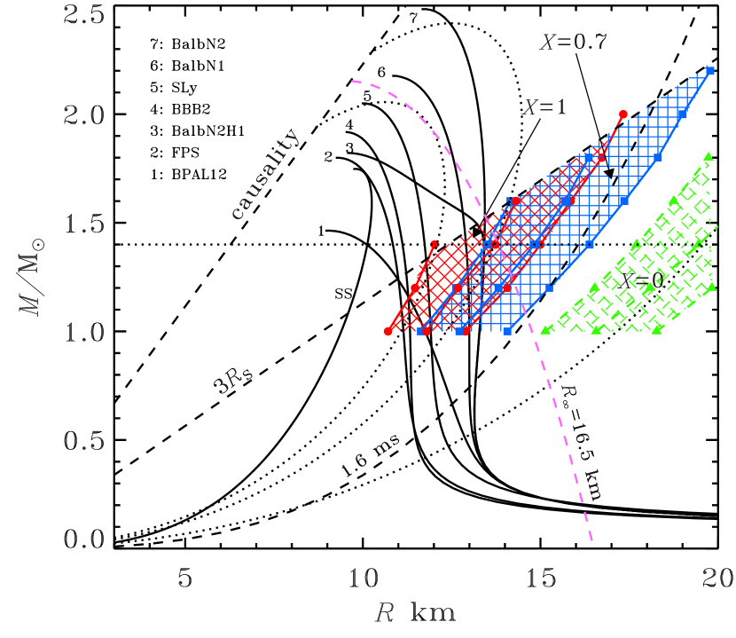
Figure 13: Permitted region (shaded) for the NS mass and radii, which can have SLs with color temperatures $2.4\pm 0.1$ keV (Gilfanov et al., 2003; Revnivtsev & Gilfanov, 2006) at luminosities similar to those observed in the Z-sources. The left shaded region (with boundaries and the centre marked by circles) is for the accreting matter containing hydrogen only, the middle one (boundaries and centre marked by squares) is for the solar composition, and the right one (marked by triangles) is for pure helium. The left boundary of each region corresponds to $T_{\rm c}=2.5$ keV, while the right boundary gives 2.3 keV. Dotted curves correspond to a simple estimation of $M-R$ relation given by equation (73) with $f_{\rm c}=1.7,\ell=0.8$ for the three chemical compositions. Various theoretical mass-radius relations for neutron and strange stars are shown for comparison (Haensel, Potekhin & Yakovlev, 2006). Dotted horizontal line corresponds to the NS mass of $1.4{\rm M}_{\odot}$. The almost vertical dashed curve corresponds to the thermally emitting NS with the apparent radius of $R_{\infty}=16.5$ km (see eq. [75] and Trümper 2005). The lower limit on the NS mass as a function of radius for a given rotational period $P$ (in ms) as derived from the NS stability $M/{\rm M}_{\odot}>0.865(R/10\ \mbox{km})^{3}P_{\rm ms}^{2}$ (Lattimer & Prakash, 2004) is presented for $P=1.6$ ms.

As we have shown above the spectrum of the SL can be represented by a diluted blackbody. The effective temperature of radiation is determined by the critical temperature from equation (3), where the left-hand side is multiplied by $\ell$, the ratio of the local flux to the critical Eddington one (reduced due to the action of the centrifugal force). The observed color temperature is $T_{\rm c}=f_{\rm c}\sqrt{1-R_{\rm S}/R}\ T_{\rm Edd}$, where corrections are made for spectral hardening and gravitational redshift. For the known color correction and $\ell$, the NS radius as a function of compactness $M/R$ can then be found from

$$R=\frac{\ell f_{\rm c}^{4}c^{3}}{2\sigma_{\rm SB}T_{\rm c}^{4}\sigma_{\rm e}}\frac{R_{\rm S}}{R}\left(1-\frac{R_{\rm S}}{R}\right)^{3/2}.$$ (73)

Assuming $f_{\rm c}=1.6-1.8$ and $\ell=0.8$, Revnivtsev & Gilfanov (2006) obtained constraints on the NS mass-radius relation (shown in Fig. 13 by dotted curves). The maximum NS radius is reached for $R_{\rm S}/R=2/5$:

$$R_{\max}=\frac{24.6}{1+X}\frac{\ell}{0.8}\left(\frac{f_{\rm c}}{1.7}\right)^{4}\left(\frac{T_{\rm c}}{2.4\ \mbox{keV}}\right)^{-4}\ \mbox{km}.$$ (74)

Here instead we calculate exactly a grid of the SL model spectra, where the main input parameters are the NS mass $M$ and radius $R$, and the SL luminosity. The NS mass is varied from 1 to 2 ${\rm M}_{\odot}$ with a step of 0.2 ${\rm M}_{\odot}$, and the NS radius is varied from 10 to 24 km with a step 1 km. Only the models with $R>3R_{\rm S}$ are considered. We take $\alpha_{\rm b}=10^{-3}$ and luminosity of $0.4L_{\rm Edd}$, and compute spectra for four inclination angles 0, 30, 60 and 90 degrees and for three chemical compositions: pure hydrogen ($X=1$), solar abundance ($X=0.7$), and pure helium ($X=0,Y=1$). The spectra are fitted by the black body and the corresponding color temperatures are found.

Models with higher He abundance have a smaller hardness factor as can be seen from equation (68). However, the local effective temperature of the SL is higher for larger He abundance (see eq. 3 and Fig. 2c). The higher $T_{\rm eff}$ leads to a higher color temperature of the integral SL spectrum. For example, at NS radius of 13 km and mass $1.4{\rm M}_{\odot}$ pure hydrogen models give color temperature of about 2.5 keV, while pure helium models produce harder spectra with $T_{\rm c}\approx 3$ keV.

Contours corresponding to the color temperature equal 2.3 (right), 2.4 (central) and 2.5 keV (left) are shown on the $M-R$ plane (Fig. 13) together with the NS models for various equations of state. These iso-temperature curves are shown for the inclination angle $i=45{\degr}$. Comparison of the observed spectra to the theoretical spectra of the SL constrains the NS radius at $13.5\pm 1.5$ km (for pure hydrogen $X=1$ model), $14.8\pm 1.5$ km (solar composition $X=0.7$) and $19\pm 1.5$ km (pure helium $X=0,Y=1$) assuming the NS mass of 1.4 solar mass. For pure hydrogen and solar abundance, the permitted radii are consistent with the hard equation of state of the NS matter. If the composition is solar, but the heavier elements are able to sink, the emitted spectra would correspond to a pure hydrogen atmosphere requiring thus smaller radii.

Increasing the inclination to $90{\degr}$ increases the deduced NS radii by about 10 per cent, while assuming $i=0{\degr}$, gives a 15 per cent reduction on $R$. The uncertainty in the luminosity increases the width of possible NS radii by about 50 per cent. Another source of uncertainty comes from the turbulence parameter $\alpha_{\rm b}$. With $\alpha_{\rm b}$ decreasing by an order of magnitude the spectrum hardens by 0.1 keV. This results in about 15 per cent decrease of the NS radius that is required to produce the observed spectra. Thus $\alpha_{\rm b}\sim 10^{-5}$ is needed to reconcile the derived NS radii with the soft equations of state (assuming solar composition). Such a small $\alpha_{\rm b}$ at the same time yields a very large column density of the SL and a rather long life-time of the accreting gas in the layer (of the order of 1 s, instead of 10 ms as in the model of IS99).

Finally, we would like to emphasize that our method of determination of the NS radius from the SL spectrum is based on the observed color temperature of radiation alone, because the SL radiates locally at almost Eddington flux. The color temperature can be related to the effective temperature which is a function of the stellar compactness (and chemical composition) as given by equation (3). This method is identical to that used for the radius-expansion X-ray bursts which are believed to reach Eddington luminosity (see e.g. Lewin, van Paradijs & Taam, 1993). In contrast to the standard methods based on the modeling of the thermal emission from the NS surface (see for example van Paradijs & Lewin, 1987; Trümper, 2005), there is no need to know precisely either the area of the emitting region, or the distance to the source.

As the standard method gives the apparent stellar radius at infinity, which is related to the NS parameters through

$$R_{\infty}=R\left(1-\frac{R_{\rm S}}{R}\right)^{-1/2},$$ (75)

the allowed band of $R$ and $M$ is nearly orthogonal to that obtained from the color temperature and equation (73) (see the almost vertical dashed curve in Fig. 13). Thus for a NS, where both the thermal emission from the surface (e.g. during the quiescence) and the BL emission (during the accretion phase) are observed, it would be possible to determine $R$ and $M$ independently. Interestingly our constraints on the NS radius are very similar to those obtained by Heinke et al. (2005) for the thermally emitting quiescent NS X7 in the globular cluster 47 Tucanae $R=14.5^{+1.8}_{-1.6}$ km. They are also consistent with the lower limit $R>14$ km obtained by Trümper (2005) for the isolated NS RX J1856-3754.

5 Conclusions

We have derived the one-dimensional equations describing the SL model on a spherical NS surface from the usual hydrodynamic equations. The obtained equations are similar to those in IS99, except for the energy conservation law where we neglected the surface density of the gravitational potential energy which is of the second order in $H/R$. This difference, however, leads only to small quantative changes. We have also implemented a pseudo-Newtonian potential to account for the main general relativity corrections and considered various chemical compositions of the accreting matter.

We have studied the vertical (radial) structure of the SL with different assumptions about the vertical distributions of the radiation flux and azimuthal velocity. The temperature structure and the emergent radiation spectra of the SL are computed accounting for the effect of Compton scattering. We showed that the local (at a given latitude) emergent spectra depend very little on details of the SL vertical structure in optically thick cases with $\Sigma_{\rm S}\gtrsim 100\ \mbox{g\ cm}^{-2}$ ($L\gtrsim 0.1L_{\rm Edd}$). These spectra can be described by the diluted Planck spectrum and are similar to the spectra of X-ray bursts with the same effective temperature and the effective surface gravity.

The integral SL spectra were computed accounting for relativistic effects such as the gravitational redshift and light bending, the relativistic Doppler effect and aberration. These spectra slightly depend on the inclination angle to the line of sight and on the SL luminosity. The local effective temperature increases with latitude, while the hardness factor $f_{\rm c}$ decreases. This leads to only slight variation of the color temperature on latitude. As a result, the integral spectra can also be well described by a single-temperature diluted Planck spectrum.

We compared our theoretical integral SL spectra with the observed spectra of the LMXRBs BLs. The observed color temperature of 2.4 $\pm$ 0.1 keV (Gilfanov et al., 2003; Revnivtsev & Gilfanov, 2006) can be reproduced for hard equations of state of NS material. Our model constrains radii of NSs in LMXRBs to 13–16 km for a 1.4 solar mass star. Soft equations of state (smaller NS radii) can be reconciled with the observed spectra only for very low viscosity $\alpha_{\rm b}\sim 10^{-5}$. Calculation of $\alpha_{\rm b}$ from the first principles is a challenging problem that deserves further attention.

References

- Barret et al. (2000) Barret D., Olive J. F., Boirin L., Done C., Skinner G. K., Grindlay J. E., 2000, ApJ, 533, 329
- Beloborodov (2002) Beloborodov A. M., 2002, ApJ, 566, L85
- Bisnovatyi-Kogan (1994) Bisnovatyi-Kogan G. S., 1994, MNRAS, 269, 557
- Done & Gierliński (2003) Done C., Gierliński M., 2003, MNRAS, 342, 1041
- Gilfanov et al. (2003) Gilfanov M., Revnivtsev M., Molkov S., 2003, A&A, 410, 217
- Grebenev & Sunyaev (2002) Grebenev S. A., Sunyaev R. A., 2002, Astron. Lett., 28, 150
- Haensel et al. (2006) Haensel P., Potekhin A. Y., Yakovlev D. G., 2006, Neutron Stars. I. Equation of State and Structure. Springer-Verlag, Dordrecht
- Heinke et al. (2005) Heinke C. O., Rybicki G. B., Narayan R., Grindlay J. E., 2005, ApJ, in press [astro-ph/0506563]
- Ibragimov et al. (2003) Ibragimov A. A., Suleimanov V. F., Vikhlinin A., Sakhibullin N. A., 2003, Astron. Rep., 47, 186
- Inogamov & Sunyaev (1999) Inogamov N. A., Sunyaev R. A., 1999, Astron. Lett., 25, 269
- Kluźniak & Wilson (1991) Kluźniak W., Wilson J. R., 1991, ApJ, 372, L87
- Kompaneets (1957) Kompaneets A. S., 1957, Sov. Phys. JETP, 4, 730
- Kurucz (1970) Kurucz R. L., 1970, SAO Special Report, 309
- Kurucz (1993) Kurucz R., 1993, CD-ROM. Smithsonian Astrophysical Observatory, Cambridge, MA
- Landau & Lifshitz (1959) Landau L. D., Lifshitz E. M., 1959, Fluid Mechanics. Pergamon Press, London
- Lattimer & Prakash (2004) Lattimer J. M., Prakash M., 2004, Sci, 304, 536
- Lewin et al. (1993) Lewin W. H. G., van Paradijs J., Taam R. E., 1993, Space Sci. Rev., 62, 223
- Madej et al. (2004) Madej J., Joss P. C., Różańska A., 2004, ApJ, 602, 904
- Mihalas (1978) Mihalas D., 1978, Stellar atmospheres, 2nd edn. W. H. Freeman and Co., San Francisco
- Mitsuda et al. (1984) Mitsuda K. et al., 1984, PASJ, 36, 741
- Pavlov et al. (1991) Pavlov G. G., Shibanov I. A., Zavlin V. E., 1991, MNRAS, 253, 193
- Popham & Narayan (1992) Popham R., Narayan R., 1992, ApJ, 394, 255
- Popham & Narayan (1995) Popham R., Narayan R., 1995, ApJ, 442, 337
- Popham & Sunyaev (2001) Popham R., Sunyaev R., 2001, ApJ, 547, 355
- Poutanen (1998) Poutanen J., 1998, in Abramowicz M. A., Björnsson G., Pringle J. E., eds, Theory of Black Hole Accretion Disks. Cambridge University Press, Cambridge, p. 100
- Poutanen & Gierliński (2003) Poutanen J., Gierliński M., 2003, MNRAS, 343, 1301
- Pringle (1977) Pringle J. E., 1977, MNRAS, 178, 195
- Pringle & Savonije (1979) Pringle J. E., Savonije G. J., 1979, MNRAS, 187, 777
- Revnivtsev & Gilfanov (2006) Revnivtsev M., Gilfanov M., 2006, A&A, in press [astro-ph/0506019]
- Shakura & Sunyaev (1988) Shakura N. I., Sunyaev R. A., 1988, Adv. Space Res., 8, 135
- Sibgatullin & Sunyaev (1998) Sibgatullin N. R., Sunyaev R. A., 1998, Astronomy Letters, 24, 774
- Sunyaev & Shakura (1986) Sunyaev R. A., Shakura N. I., 1986, Sov. Astr. Let., 12, 117
- Swartz et al. (2002) Swartz D. A., Ghosh K. K., Suleimanov V., Tennant A. F., Wu K., 2002, ApJ, 574, 382
- Trümper (2005) Trümper J., 2005, in Baykal A., Yerli S.K., Inam S.C., Grebenev S., eds, NATO Science Series II: Mathematics, Physics and Chemistry, Vol. 210, The Electromagnetic Spectrum of Neutron Stars. Springer-Verlag, Dordrecht, p. 117 [astro-ph/0502457]
- Tylenda (1981) Tylenda R., 1981, Acta Astron., 31, 267
- van der Klis (2000) van der Klis M., 2000, ARA&A, 38, 717
- van Paradijs & Lewin (1987) van Paradijs J., Lewin W. H. G., 1987, A&A, 172, L20
- Verner et al. (1996) Verner D. A., Ferland G. J., Korista K. T., Yakovlev D. G., 1996, ApJ, 465, 487
- Zavlin & Shibanov (1991) Zavlin V. E., Shibanov Y. A., 1991, Sov. Astron., 35, 499