The magnetic field and confined wind of the O star $\theta^{1}$ Orionis C

Abstract

Aims. In this paper we confirm the presence of a globally-ordered, kG-strength magnetic field in the photosphere of the young O star $\theta^{1}$ Orionis C, and examine the properties of its optical line profile variations.

Methods. A new series of high-resolution MuSiCoS Stokes $V$ and $I$ spectra has been acquired which samples approximately uniformly the rotational cycle of $\theta^{1}$ Orionis C. Using the Least-Squares Deconvolution (LSD) multiline technique, we have succeeded in detecting variable Stokes $V$ Zeeman signatures associated with the LSD mean line profile. These signatures have been modeled to determine the magnetic field geometry. We have furthermore examined the profile variations of lines formed in both the wind and photosphere using dynamic spectra.

Results. Based on spectrum synthesis fitting of the LSD profiles, we determine that the polar strength of the magnetic dipole component is $1150\la B_{\rm d}\la 1800$ G and that the magnetic obliquity is $27\degr\la\beta\la 68\degr$, assuming $i=45\pm 20\degr$. The best-fit values for $i=45\degr$ are $B_{\rm d}=1300\pm 150\ (1\sigma)$ G and $\beta=50\degr\pm 6\degr\ (1\sigma)$. Our data confirm the previous detection of a magnetic field in this star, and furthermore demonstrate the sinusoidal variability of the longitudinal field and accurately determine the phases and intensities of the magnetic extrema. The analysis of “photospheric” and “wind” line profile variations supports previous reports of the optical spectroscopic characteristics, and provides evidence for infall of material within the magnetic equatorial plane.

1 Introduction

The detection of magnetic fields in O-type stars has proven to be a remarkably challenging observational problem (e.g., Donati et al. 2001). The apparent absence of magnetic signatures has often been interpreted as a selection effect, since about 5% of B- and A-type stars (see, e.g., Johnson 2005) do display organized magnetic fields with disk-averaged strengths ranging from a few hundred G to several tens of kG (Mathys 2001). These fields are believed to be the fossil remnants of either interstellar fields swept up during the star formation process or fields produced by a pre-main sequence envelope dynamo that has since turned off. As there is no particular reason to suspect that similar processes should not occur during the formation of more massive stars, it seems reasonable a priori to expect that magnetic fields of similar structure and intensity should also exist in O-type stars.

In the absence of direct magnetic measurements, this view has been supported by the wide-spread occurrence of variability in the winds of O-type stars, which may provide indirect evidence for the presence of dynamically important magnetic fields in their atmospheres. During the past 20 years, sustained optical and UV spectroscopic observations have shown that the winds of O-type stars are highly structured, exhibiting both coherent and stochastic behaviour, as well as cyclical variability on timescales ranging from hours to days. A key result of this work has been the conclusion that a major component of this variability results from rotational modulation of structures imposed on the wind by some deep-seated process. Magnetic fields are presently considered a likely source of such structures (e.g. (Cranmer & Owocki 1996)).

Although by no means prototypical, $\theta^{1}$ Orionis C (HD 37022; HR 1895) is perhaps the best example of an O-type star with distinctive, periodic variability of its spectroscopic stellar wind features. It is a very young, peculiar $\sim$O7 star, and the brightest and hottest member of the Orion Nebula Cluster. It exhibits strictly periodic spectroscopic variability which is strongly suggestive of a magnetic rotator: H$\alpha$ and He ii $\lambda$4686 emission, peculiar ultraviolet C iv $\lambda\lambda$1548, 1550 wind lines, photospheric absorption lines, and ROSAT X-ray emission all appear to vary with a single well-defined period of $15.422\pm 0.002$ d (Stahl et al. 1993, 1996; Walborn & Nichols 1994; Gagné et al. 1997). The similarity of this behaviour to that of some magnetic A- and B-type stars (see, e.g., Shore & Brown 1990) has motivated the suggestion first made by Stahl et al. (1996) that $\theta^{1}$ Ori C also hosts a fossil magnetic field which confines the stellar wind and produces the observed variability by rotational modulation. Such a phenomenon appears to have been first suggested (for the O star $\zeta$ Pup) by Moffat & Michaud (1981) (although no field has ever been detected in that star).

In order to test this suggestion, Donati & Wade (1999) obtained longitudinal magnetic field measurements of $\theta^{1}$ Ori C, but failed to detect the presence of a photospheric field. However, in a seminal paper, Donati et al. (2002) reported the detection of a fossil magnetic field in the photosphere of $\theta^{1}$ Ori C based on 5 measurements of the Stokes $V$ profiles of selected photospheric absorption lines. This detection provided the first empirical support that dynamically important magnetic fields exist in O-type stars, and that their behaviour is directly linked to spectroscopic variability. It also represents the youngest main sequence star in which a fossil-type field has been detected (comparable in age to NGC 2244-334; Bagnulo et al. 2004). Since $\theta^{1}$ Ori C is clearly a pivotal object, it is important that this detection be corroborated and the determination of its magnetic properties be refined.

The primary goal of the present paper is to report confirmation of the detection of a magnetic field in the photospheric lines of $\theta^{1}$ Ori C. Our new spectropolarimetric observations, which provide a substantially larger data set that samples the $15\aas@@fstack{d}422$ rotational period more fully, are described in §2. The analysis of the Least-Squares Deconvolved circular polarisation spectra, both in terms of the mean longitudinal magnetic field, $\langle B_{z}\rangle$, and the LSD mean Stokes $V$ profiles, is described in §3. In §4 we discuss the variability characteristics of features in the Stokes $I$ spectrum, and comment on consistency with both the magnetically-confined wind shock model of Donati et al. (2002) as well as very recent MHD simulations of magnetically-channelled winds by ud-Doula & Owocki (2002) and Gagné et al. (2005). Finally, in §5 we summarise our results, and discuss implications for our understanding of the origin and evolution of magnetic fields in intermediate- and high-mass stars, and for our understanding of wind modulation in massive stars.

2 Observations

Circular polarisation (Stokes $V$) spectra of $\theta^{1}$ Ori C were obtained during the period 1997-2000 using the MuSiCoS spectropolarimeter mounted on the 2 metre Bernard Lyot telescope at Pic du Midi observatory. The spectropolarimeter consists of a dedicated polarimetric module mounted at the Cassegrain focus of the telescope and connected by a double optical fibre (one for each orthogonal polarisation state) to the table-mounted cross-dispersed échelle spectrograph. The spectrograph and polarimeter module are described in detail by Baudrand & Bohm (1992) and by Donati et al. (1999), respectively. The standard instrumental configuration allows for the acquisition of circular or linear polarisation spectra with a resolving power of about 35,000 throughout the range 4500-6600 Å.

Table 1: Journal of observations. Phases are calculated according to the ephemeris of Stahl et al. (1996), ${\rm JD}=2448833.0+15.422\,{\rm E}$. The peak S/N per pixel in the continuum is quoted in the final column.

No.	Date			HJD	Phase	$t_{\rm exp}$	S/N
				($-$2450000)		[minutes]	pixel-1
01	1997	Feb	20	0500.3453	0.1147	40	280
02	1997	Feb	22	0502.3429	0.2442	40	450
03	1997	Feb	23	0503.3230	0.3078	40	140
04	1997	Feb	25	0505.3160	0.4370	40	300
05	1998	Feb	15	0860.4021	0.4616	40	250
06	1998	Feb	26	0871.3354	0.1706	40	270
07	2000	Feb	03	1578.4219	0.0198	40	250
08	2000	Feb	03	1578.4536	0.0218	40	240
09	2000	Feb	04	1579.3932	0.0828	40	250
10	2000	Feb	04	1579.4235	0.0847	40	270
11	2000	Feb	04	1579.4539	0.0867	40	320
12	2000	Feb	12	1587.3739	0.6003	40	340
13	2000	Feb	15	1590.3822	0.7953	40	310
14	2000	Feb	15	1590.4131	0.7973	40	260
15	2000	Feb	21	1596.3907	0.1849	40	270
16	2000	Feb	21	1596.4211	0.1869	40	370
17	2000	Feb	21	1596.4518	0.1889	40	350
18	2000	Feb	22	1597.3515	0.2472	40	410
19	2000	Feb	22	1597.3823	0.2492	40	400
20	2000	Feb	22	1597.4133	0.2512	40	410
21	2000	Feb	22	1597.4439	0.2532	40	380
22	2000	Feb	24	1599.3534	0.3770	40	410
23	2000	Feb	24	1599.3840	0.3790	40	400
24	2000	Feb	24	1599.4156	0.3811	40	340
25	2000	Feb	25	1600.3465	0.4414	40	410
26	2000	Feb	25	1600.3780	0.4435	40	410
27	2000	Feb	25	1600.4105	0.4456	40	390
28	2000	Feb	26	1601.3610	0.5072	40	340
29	2000	Feb	26	1601.3922	0.5092	40	340
30	2000	Feb	26	1601.4229	0.5112	40	310
31	2000	Feb	27	1602.3490	0.5713	40	360
32	2000	Feb	27	1602.3881	0.5738	40	350
33	2000	Feb	27	1602.4191	0.5758	40	310
34	2000	Feb	28	1603.3767	0.6379	40	240
35	2000	Feb	28	1603.4077	0.6399	40	300
36	2000	Feb	28	1603.4391	0.6420	40	230
37	2000	Mar	02	1606.3531	0.8309	40	340
38	2000	Mar	02	1606.3844	0.8329	40	390
39	2000	Mar	02	1606.4161	0.8350	40	340
40	2000	Mar	04	1608.3696	0.9617	40	470
41	2000	Mar	04	1608.4005	0.9637	40	410
42	2000	Mar	04	1608.4311	0.9657	40	360
43	2000	Mar	05	1609.3605	0.0259	40	350
44	2000	Mar	05	1609.3910	0.0279	40	310
45	2000	Mar	05	1609.4216	0.0299	40	260

A complete circular polarisation observation consists of a series of 4 sub-exposures between which the polarimeter quarter-wave plate is rotated back and forth between position angles (of the plate fast axis with respect to the polarising beamsplitter fast axis) of $-45\degr$ and $+45\degr$. This procedure results in exchanging the orthogonally polarised beams throughout the entire instrument, which makes it possible to reduce systematic errors (due to interference and other effects in the telescope and polarisation optics, instrumental drifts, astrophysical variability, etc.) in spectral line polarisation measurements of sharp-lined stars to below a level of about $10^{-4}$ (Wade et al. 2000).

In total, 45 Stokes $V$ spectra of $\theta^{1}$ Ori C were obtained over 4 observing runs in 1997 February, 1998 February/March, 2000 February/March, and 2000/2001 December/January, with peak signal-to-noise ratios (S/N) of typically 250 per pixel in the continuum. The 6 spectra obtained during 1997 and 1998 have already been discussed by Donati & Wade (1999). Some fringing is visible in the Stokes $I$ spectra (maximum amplitude $\sim$ 1% peak-to-peak in the red), although no fringing is evident in Stokes $V$. Such effects are present in most polarimeters, and generally result from internal reflections producing secondary beams coherent with the incident beam, but with important (wavelength dependent) phase differences (Semel 2003). This fringing limits the effective S/N of the Stokes $I$ spectra to about 150:1 at H$\alpha$, and to about 350:1 at He ii $\lambda 4686$.

In addition to exposures of $\theta^{1}$ Ori C, during each run observations of various magnetic and non-magnetic standard stars were obtained which confirm the nominal operation of the instrument (see, e.g., Shorlin et al. 2002). The observing log is shown in Table 1.

3 Least-Squares Deconvolution

As demonstrated by, e.g., Donati & Wade (1999), the Least-Squares Deconvolution (LSD) multi-line procedure can provide enormous improvement in the precision of spectral line polarisation measurements as compared with individual line measurements. We began using the 13 lines employed by Donati & Wade (1999) for the LSD analysis. After exploring the effect of removing lines from this list, it became clear based on the shape of the Stokes $I$ profile that only 3 of the lines in the mask were contributing relatively uncontaminated photospheric profiles. In the end, an LSD mask including only O iii $\lambda$5592, C iv $\lambda$5801 and C iv $\lambda$5811 was used, with a mean wavelength $\bar{\lambda}=5730$ Åand a mean Landé factor $\bar{z}=1.18$. We found that the resultant LSD S/N was dependent on the velocity bin size of the extracted LSD profiles. Ultimately, experiment yielded a best S/N for an bin size of 13.5 km s^-1. Therefore, each pixel in the extracted Stokes $I$ and $V$ LSD profiles corresponds to a velocity interval of 13.5 km s^-1. Each extracted LSD profile was determined from 4 individual photospheric features (C iv $\lambda$5801 appears in two separate orders in each spectrum).

To further reduce the noise, LSD profiles were binned in phase, according to the 15.422 day period of Stahl et al. (1996), weighting each pixel according to the inverse of its squared error bar. The final binned profiles, which will be used for all further LSD analysis, are summarised in Table 2.

Table 2: Binned LSD Stokes $V$ profiles and longitudinal magnetic field measurements

Mean	Binned	$\langle B_{z}\rangle\pm\sigma_{B}$	NLSD
Phase	Spectra	(G)	(%)
0.0550	01,07-09,10,11,43-45	$480\pm 95$	$3.97\,10^{-2}$
0.1829	06,15-17	$590\pm 133$	$5.38\,10^{-2}$
0.2491	02,18-21	$334\pm 96$	$3.74\,10^{-2}$
0.3613	03,22-24	$120\pm 130$	$5.04\,10^{-2}$
0.4459	04,05,25-27	$-110\pm 118$	$4.27\,10^{-2}$
0.5415	28-33	$130\pm 110$	$4.12\,10^{-4}$
0.6301	12,34-36	$-96\pm 164$	$5.99\,10^{-2}$
0.7964	13,14	$14\pm 226$	$8.41\,10^{-2}$
0.8330	37-39	$340\pm 153$	$5.67\,10^{-2}$
0.9637	40-42	$589\pm 116$	$4.89\,10^{-2}$

Figure 1: Longitudinal magnetic field variation (in G) of $\theta^{1}$ Ori C phased according to the ephemeris described in the text. Upper panel – measurements from Stokes $V$ profiles; Lower panel – measured from diagnostic $N$ (null) profiles

4 Magnetic field geometry

Following the approach of Donati et al. (2001), the best-fit geometry of the dipolar magnetic field was determined using two complementary procedures.

First we modeled the variation of the mean longitudinal magnetic field. The longitudinal field $\langle B_{z}\rangle$ and its associated error $\sigma_{B}$ were inferred from each set of LSD profiles, in the manner described by Donati et al. (1997) and modified by Wade et al. (2000). Measurements were made in the range $\pm 80$ km s^-1 around line centre, in both the Stokes $V$ and diagnostic $N$ LSD profiles. The $N$, or null profiles are calculated from analysis of Stokes $V$ CCD frames obtained at identical waveplate angles, and are nominally consistent with zero (see, e.g., Donati et al. 1997). The $N$ profiles provide a powerful diagnosis of systematic errors in the polarisation data. The measurements are summarised in Table 2 and are shown, phased according to the 15.422 d period, in Fig. 1. The reduced $\chi^{2}$ of the (phased) Stokes $V$ measurements of $\langle B_{z}\rangle$ is 1.0 for a first-order sine fit (fitting zero-point, amplitude and phase), and 10.2 for the null-field hypothesis (i.e. a straight line through $\langle B_{z}\rangle=0$. The reduced $\chi^{2}$ of the $N$ $\langle B_{z}\rangle$ measurements is 0.8 for a first-order sine fit (fitting zero-point, amplitude and phase), and 1.2 for the null-field hypothesis. Based on these results, for the 10 longitudinal field data discussed here, the null-field hypothesis can be confidently ruled out for the Stokes $V$ $\langle B_{z}\rangle$ variation (false-alarm probability $\ll$ 0.1%), whereas a null magnetic field is consistent with the $N$ measurements within 2$\sigma$.

The 1^st-order sine fit to the Stokes $V$ $\langle B_{z}\rangle$ data is characterised by a maximum of $550\pm 85$ G, a minimum of $-35\pm 85$ G and a phase of maximum $\phi_{0}=0.05\pm 0.05$ (all uncertainties $1\sigma$).

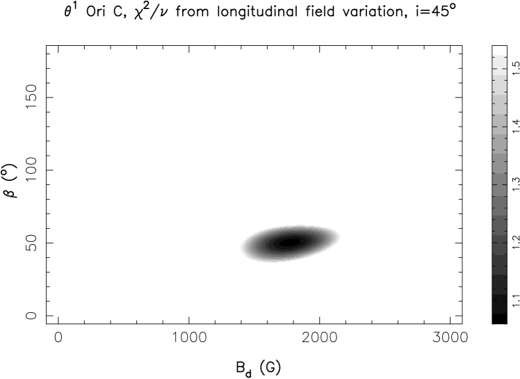
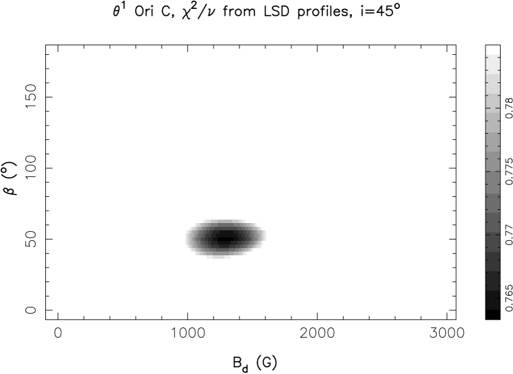
Figure 2: Map of reduced $\chi^{2}$s of model fits to $\theta^{1}$ Ori C longitudinal field variation (top) and to LSD profiles (bottom) assuming $i=45\degr$. Reduced $\chi^{2}$ intervals corresponding to 95% confidence [approximately $2\sigma$) are computed using the $\chi^{2}$ probability tables of Bevington (1969).

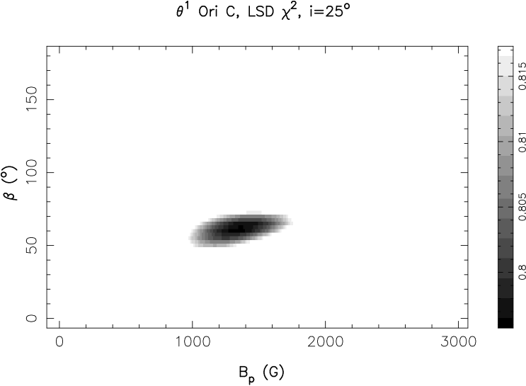
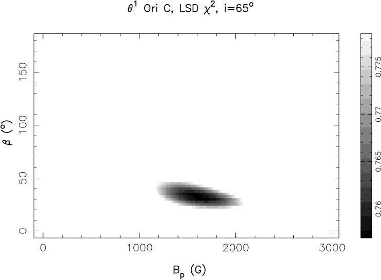
Figure 3: Map of reduced $\chi^{2}$s of model fits to $\theta^{1}$ Ori C LSD profiles assuming $i=25\degr$ and $i=60\degr$. Reduced $\chi^{2}$ intervals corresponding to 95% confidence are computed using the $\chi^{2}$ probability tables of Bevington (1969).

Figure 4: Averaged Stokes $I$ and $V$ and diagnostic null ($N$) LSD profiles of $\theta^{1}$ Ori C, compared with profiles computed assuming the best-fit dipole model.

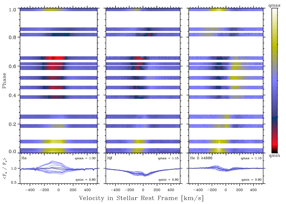
Figure 5: Dynamic spectra illustrating the line profile variations of circumstellar features as a function of phase of the 15.422-day period. Quotient spectra computed by dividing each spectrum in the time series by the mean spectrum are illustrated. The original spectral time series is also overplotted in the lower panel, where the mean spectrum is shown in black. Note that different lines have different dynamic ranges (“stretches”). These are indicated by qmax and qmin, which are the maximum and minimum values of the quotient that are plotted, respectively. White (qmax) corresponds to wavelengths or times when the local flux is greater than its mean value. Strong nebular emission components have been excised from the central region of H$\alpha$ and H$\beta$ by interpolating linearly over $\sim$100 km s^-1 (for H$\alpha$) or $\sim$50 km s^-1 (for H$\beta$).

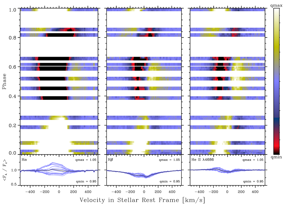
Figure 6: Same as Fig. 5, with a small dynamic range (“stretch’) that is fixed for all features. This presentation emphasizes weak spectral features like the red-shifted emission near phase 0.5.

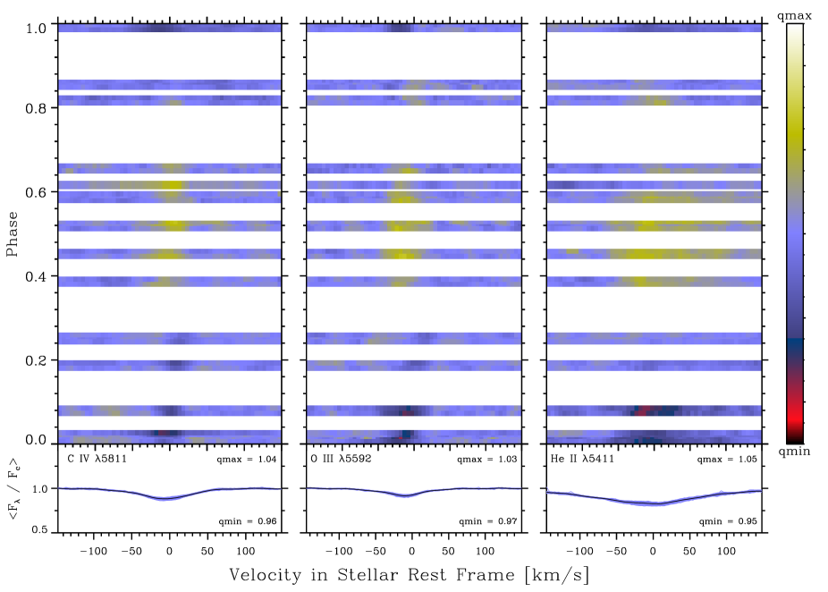
Figure 7: Same as Fig. 5, only for a selection of features predominantly formed in the photosphere of $\theta^{1}$ Ori C.

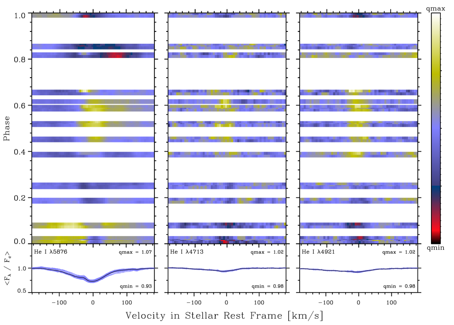
Figure 8: Same as Fig. 5, only for a selected He i lines. A strong nebular emission component has been excised from the central region of He i $\lambda$5876.

Then, using a modified version of the programme Fldcurv, we calculated model longitudinal field variations corresponding to a large number of dipolar magnetic field configurations, varying the dipole intensity $B_{\rm d}$ as well as the obliquity angle $\beta$. Fldcurv computes the surface distribution of magnetic field corresponding to a particular magnetic geometry, then weights and integrates the longitudinal component over the hemisphere of the star visible at a given phase (for this procedure we have assumed a limb-darkening coefficient of 0.4).

In order to uniquely identify the magnetic geometry, we must specify four parameters: The magnetic dipole polar strength $B_{\rm d}$, the inclination of the stellar rotational axis to the observer’s line-of-sight $i$, the obliquity of the magnetic axis with respect to the rotational axis $\beta$, and the phase of closest passage of the positive magnetic pole to the line-of-sight, $\phi_{0}$. The phase variation of the longitudinal field allows us to constrain 3 of these parameters; typically $B_{\rm d},\beta$ and $\phi_{0}$ are determined by fitting the magnetic curve, whereas $i$ is constrained using other data. Donati et al. (2002) derive $i=45\pm 20\degr$ based on the rotational period and inferred $v\sin i$ of $\theta^{1}$ Ori C, as well as the characteristics of the optical and UV spectroscopic variability. Their conclusions are independently supported by the optical spectroscopic study of Simón-Díaz et al. (2005), who find $i=44\pm 12\degr$, and qualitatively by the original Magnetically-Confined Wind Shock modelling of the X-ray variation of this star by Babel & Montmerle (1997b). We therefore adopt $i=45\pm 20\degr$ for the modelling performed in this paper.

For each computed model (over 40,000 in total), the reduced $\chi^{2}$ of the model fit to the observations was calculated. The ’map’ of these $\chi^{2}$s, shown in the upper frame of Fig. 2 (where black regions represent acceptable models, whereas white regions represent models rejectable at more than the 95% [approximately 2$\sigma$] confidence level), indicates that for a rotational axis inclination $i=45\degr$, acceptable magnetic models are characterised by $B_{\rm d}=1900\pm 250$ G and $\beta=50\pm 8\degr$ (where associated uncertainties are quoted at 1$\sigma$). If we allow a $20\degr$ uncertainty in our assumed value of $i$, we obtain $B_{\rm d}=2400\pm 300$ G and $\beta=30\pm 8\degr$ ($i=65\degr$) and $B_{\rm d}=2600\pm 450$ G and $\beta=67\pm 5\degr$ ($i=25\degr$). Therefore our modeling of the longitudinal field variation constrains the dipole magnetic field geometry of $\theta^{1}$ Ori C to $1650\la B_{\rm d}\la 3050$ G and $22\degr\la\beta\la 73\degr$.

Our second procedure involves direct modeling of the LSD Stokes $I$ and $V$ profiles, in a manner similar to that described first by Donati et al. (2001). In particular, all line profile modeling was accomplished using the LTE polarised synthesis code Zeeman2 (Landstreet 1988; Wade et al. 2001) and assuming an Atlas9 model atmosphere with $T_{\rm eff}=40,000$ K and $\log g=4.0$.

We began by finding a phase-independent model fit to the Stokes $I$ profiles, varying the line equivalent width, projected rotational velocity $v\sin i$, and microturbulent broadening $\zeta$ as free parameters. Assuming $v\sin i=20$ km s^-1 (Donati et al. 2002), we found a microturbulent broadening $\zeta=30$ km s^-1 (corresponding to a total thermal$+$turbulent broadening of about 31 km s^-1) provided a best-fit to the profiles. As reported by Donati et al. (2002), the LSD Stokes $I$ profiles vary systematically according to rotational phase, with a maximum depth of about 12% of the continuum at phase 0.0, and a minimum depth of about 9% of the continuum at phase 0.5. This variation is quite probably related to variable contamination of the photospheric profiles by the wind spectrum; see §5.

The next step was to calculate Stokes $V$ profiles corresponding to a large number of dipole surface magnetic field configurations, varying the dipole parameters $\beta$ and $B_{\rm d}$ for selected values of $i$. Finally, we compared each of these calculated profiles (about 28,000 in all) with the observed Stokes $V$ profile, calculating the reduced $\chi^{2}$ and building up a “map” of their agreement as well.

The results are illustrated in the lower frame of Fig. 2 (for $i=45\degr$) and in Fig. 3 (for $i=25\degr$ and $i=65\degr$) for 95% (2$\sigma$) confidence. For $i=45\degr$, we obtain a somewhat smaller value for the intensity of the best-fit dipole, $B_{\rm d}=1300\pm 150$ G, and $\beta=50\degr\pm 6\degr$ (again, all quoted uncertainties are $1\sigma$). For $i=25\degr$ we obtain $B_{\rm d}=1350\pm 150$ G and $\beta=62\degr\pm 6\degr$, while for $i=65\degr$ we obtain $B_{\rm d}=1600\pm 200$ G and $\beta=33\degr\pm 6\degr$. Therefore our modeling of the LSD mean Stokes profile variation constrains the dipole magnetic field geometry of $\theta^{1}$ Ori C to $1150\la B_{\rm d}\la 1800$ G and $27\degr\la\beta\la 68\degr$. The reduced $\chi^{2}$ for the null-field hypothesis for the $V$ measurements is 1.11, versus 0.76 for the best-fit dipole model, indicating that the null-field hypothesis can be confidently ruled out for the Stokes $V$ spectrum (false-alarm probability $\ll$ 0.1%). At the same time, a similar analysis of the $N$ diagnostic null LSD profiles provides a best-fit model of $B_{\rm d}=150\pm 225$ G with reduced $\chi^{2}$ of 0.69, consistent with a null field and indicating that no significant fringing contamination of the $N$ profiles exists.

The low reduced $\chi^{2}$ statistics obtained for both Stokes $V$ and $N$ suggest that the error bars are slightly overestimated (by about 10%). Based on the results of Wade et al. (2000), this is not unexpected. Moreover, the difference in best-fit reduced $\chi^{2}$ obtained for the $V$ versus the $N$ profiles (0.76 versus 0.69) is marginally significant, indicating that (not surprisingly) the Stokes $V$ signatures are not quite fit to within their error bars, and suggesting that other unmodelled effects may be at play. The computed Stokes profiles corresponding to the best-fit model are compared with the mean LSD profiles in Fig. 3.

The general solutions for the magnetic field geometry obtained using these two methods are in good agreement. The $B_{\rm d}$ solutions for $i=45\degr$ differ at the 1.5$\sigma$ level. Although not especially significant, this difference could be attributable to the more approximate weighting of the local field in the Fldcurv model, or possibly contributions to the amplitude and variability of the Stokes $V$ signatures by emission contamination of the photospheric profiles by the circumstellar material.

Due to the more sophisticated nature of the direct Stokes $V$ fitting procedure, we adopt these results as our formal constraints on the surface magnetic field of $\theta^{1}$ Ori C. These results are perfectly consistent with those derived by Donati et al. (2002), but are to be preferred since they are derived from a larger sample of spectra. We therefore confirm the detection and the geometrical characteristics of the magnetic field discovered by Donati et al. (2002). Moreover, we can affirm the sinusoidal nature of the longitudinal field variation and confidently define the phases of maximum and minimum $\langle B_{z}\rangle$ ($0.05\pm 0.05$ and $0.55\pm 0.05$, respectively) according to the ephemeris of Stahl et al. (1996).

The geometry of the magnetic field and circumstellar material of $\theta^{1}$ Ori C  is sketched in Fig. 1 of Smith & Fullerton (2005) or Gagné et al. (2005), and is illustrated as a series of animations at www.astro.udel.edu/t1oc.

5 Line-profile variations

Phase-resolved variations of the Stokes $I$ profiles from the 2000 time series are displayed in an image format for selected transitions in Figures 5–8. In these images, which are commonly referred to as “dynamic spectra”, individual spectra occupy horizontal strips, which are stacked vertically to show systematic variations with time. The transitions are grouped to illustrate variations that are predominantly circumstellar (Fig. 5 and 6) and photospheric (Fig. 7), with selected He i lines serving as hybrid cases (Fig. 8).

The line-profile variations of $\theta^{1}$ Ori C have been previously illustrated as dynamic spectra by Stahl et al. (1996, for H$\alpha$, He ii $\lambda$4686, C iv $\lambda\lambda$1548, 1550, Si iv $\lambda\lambda$ 1393, 1402, and O iii $\lambda$5592) and by Reiners et al. (2000, for He i $\lambda$4471 and $\lambda$4713, C iv $\lambda$5811, and O iii $\lambda$5592). Stahl et al. (1996) represented the variations as differences with respect to either (a) line profiles from a similar star [15 Monocerotis; spectral type O7 V((f))] that are at most modestly contaminated by stellar-wind emission; or (b) minimum absorption profiles from the time series. Reiners et al. (2000) illustrated the variations in the spectra themselves, i.e., without renormalizing by a template spectrum. In contrast, the dynamic spectra illustrated here represent variations with respect to the mean spectrum, which is reasonably well defined by the approximately uniform sampling of this time series. The advantage of displaying quotient spectra with respect to the mean profile is that the relative amplitude of variations can be compared in a meaningful way between (unsaturated) lines of different shape and strength. Whatever template is used to normalize a time series, it is worth remembering that the emergent spectrum is a very nonlinear function of, e.g., hydrodynamic variables such as density. Consequently, quantitative interpretation of the line profile variations in terms of physical parameters generally requires comparison with a model.

5.1 Circumstellar lines

Figures 5 and 6 illustrate the line-profile variations for H$\alpha$, H$\beta$, and He ii $\lambda$4686, all of which are dominated by stellar wind material in the magnetosphere. All three lines exhibit qualitatively similar patterns of variability. In Fig. 5, the contrast is adjusted separately for each line in order that the entire variation can be seen, while in Fig. 6 a fixed high-contrast “stretch” is used to enhance the visibility of weaker variations.

Fig. 5 confirms that the basic modulation consists of a broad emission excess that attains maximum strength at phase 0.0 (when the magnetic equator is viewed approximately face-on), decreases to a minimum near phase 0.5 (when the magnetic equator is viewed approximately edge-on), and increases again starting near phase 0.75. Although the overall symmetry of the emission feature is difficult to determine due to contamination from the nebular component in H$\alpha$ and H$\beta$, it is blue-shifted near phase 0 by perhaps as much as 100 km s^-1. As the emission fades, the primary variations are more nearly centered on the rest velocity of the star.

However, Fig. 6 also indicates the presence of a second component, which is particularly prominent in He ii $\lambda$4686. It consists of an approximately stationary excess with respect to the template at $v_{r}\approx 200$ km s^-1 between phases $\sim$0.4 and 0.6, which achieves maximum strength near phase 0.5 (i.e., when the magnetic equator is viewed edge-on). Although it is often difficult to determine whether an increase in the quotient spectrum represents excess emission or reduced absorption with respect to the template spectrum, it is clear from examination of the line profiles themselves that this component is due to emission. This component has been noted previously in H$\alpha$ by Stahl et al. (1993), who concluded that it was responsible for the smaller minimum near phase 0.5 in the “M-shaped” equivalent width curve; see, e.g., Fig. 4 of Stahl et al. (1996). However, the origin of this feature was not discussed.

5.2 Photospheric lines

Fig. 7 shows the line-profile variations of “photospheric” lines, i.e., lines that are not obviously contaminated by emission from the stellar wind or material trapped in the magnetosphere. The lines included in this category are C iv $\lambda\lambda$5801, 5811, O iii $\lambda$5592, and He ii $\lambda$5411. The first three of these are combined to obtain the LSD measurements of the magnetic field of $\theta^{1}$ Ori C.

The variations in all these lines are qualitatively similar, including C iv $\lambda$5801, which is not illustrated. They are deeper with respect to the mean profile between phases 0.0 and $\sim$0.15; less deep between phases 0.2 and 0.6 (possibly later); and deeper again between phases $\sim$0.8 and 1.0. As previously noted by Stahl et al. (1996), the variations appear to move from blue-to-red (i.e., in the sense of rotation), particularly near phase 0, but are confined to the central region of the line profile. The behaviour illustrated here is very similar to that exhibited in other dynamic spectra, despite differences in the templates used; see, e.g., Stahl et al. (1996) and Reiners et al. (2000).

Although not illustrated here, several other high-excitation lines were also investigated. No significant variations were visible in the He ii $\lambda$4542 and Si iv $\lambda$4654 absorption lines or the C iii $\lambda$5696 selective emission feature. A weak modulation might be present in Si iv $\lambda$4631.

5.3 He i lines

The line profile variations of the He i lines illustrated in Fig. 8 span the behaviour of “wind” and “photospheric” lines. In particular, the strong He i $\lambda$5876 triplet exhibits “circumstellar” variations. This is not surprising, since the sensitivity of He i $\lambda$5876 to low-density environments is a well-known consequence of non-LTE physics. However, the “circumstellar” variations in He i $\lambda$5876 occur at smaller velocities than indicated in Fig. 5.

In contrast to He i $\lambda$5876, the weaker He i $\lambda$4713 triplet and $\lambda$4921 singlet show “photospheric” variations that are very similar in phasing and character to those illustrated in Fig. 7. The variations in He i $\lambda$4713 are substantially weaker than those in He i $\lambda$4921, even though the lines themselves have similar strength. Although not illustrated here, the He i $\lambda$5015 singlet also shows weak “photospheric” variations.

5.4 Origin of the line profile variations

The primary modulation of the circumstellar line profiles has been modelled by Donati et al. (2002) in terms of the “magnetically confined wind shock model” of Babel & Montmerle (1997b, a). The key feature of this model is that a sufficiently strong, dipolar magnetic field channels wind material to the magnetic equator, where it collides with material similarly channeled from the opposite hemisphere. The consequences include substantial shock heating of the gas, the development of extended cooling zones, and the creation of a zone of enhanced density at the magnetic equator. With this model and their revised mapping between rotational and magnetic phase (which we confirm), Donati et al. (2002) were able to reproduce the fundamental features of the primary modulation; see, e.g., their Fig. 12. As a result, the maximum emission from circumstellar material is now understood to come from the cooling region above and below the magnetic equator, which is viewed face-on at phase 0.0. In contrast, the observer views the magnetic equatorial plane edge-on at phase 0.5, at which time the cooling disk is viewed edge-on against the stellar photosphere and its contributions to the H$\alpha$ profile are minimized. Despite the generally good fit, Donati et al. (2002) noted some difficulties with their model profiles, which also did not reproduce the red-shifted emission feature near phase 0.5

Recently, Gagné et al. (2005) presented a magnetohydrodynamic (MHD) model of the wind of $\theta^{1}$ Ori C that confirms and extends the basic picture provided by the “magnetically confined wind shock” model. The new “magnetically channeled wind shock” model follows the same computational approach described by ud-Doula & Owocki (2002) by allowing for the dynamic competition between the outward forces of radiation pressure and the channeling and confinement of the magnetic field. However, in addition to allowing for the feedback of the outflow on the geometry of the magnetic field, the newer model also incorporates a detailed treatment of the energy balance in the wind, including the effects of compressive heating due to the strong shocks in the vicinity of the magnetic equator. Gagné et al. (2005) show that this model successfully explains both the periodic modulation of X-ray emission exhibited by $\theta^{1}$ Ori C and the basic features of the X-ray emission lines.

The new MHD model also suggests that the circumstellar environment of $\theta^{1}$ Ori C is much more dynamic than previously supposed. In particular, the models show that the amount of material confined to the region of the cooling disk is limited by outflow through the disk beyond the Alfvén radius (i.e., the point at which the magnetic field can contain material channeled to the region of the magnetic equator) as well as infall in the inner regions. This infall occurs sporadically when cool, compressed material in the magnetic equator becomes too dense to be supported by radiative driving, and consequently falls back onto the stellar surface along distorted field lines. Although much of the infalling material is too cool to emit X-rays, Gagné et al. (2005) found evidence that the radial velocities of X-ray emission lines were systematically red-shifted by as much as 93 km s^-1 when the disk was viewed edge on (i.e., near phase 0.5)

Smith & Fullerton (2005) also recognized that the presence of infalling material near the magnetic equator provides a clue to the origin of the red-shifted emission feature near phase 0.5 in line profiles dominated by circumstellar material (Fig. 6). They attributed this feature to a column of optically thick material flowing inward at the magnetic equator, and used this interpretation to explain previously unnoticed modulations of the C iv and N v resonance doublets at modest red-shifts of 250 km s^-1 or less. We similarly attribute the red-shifted emission features near phase 0.5 in Fig. 6 (and also for He i $\lambda$5876 in Fig. 8) to the infalling material seen in the MHD models. In this context, the fact that the emission feature is seen at smaller red-shifted velocities in He i $\lambda$5876 ($\sim$50 km s^-1; possibly over a smaller range of phases) than its counterpart in He ii $\lambda$4686 ($\sim$200 km s^-1) suggests that He⁺ is formed closer to the radius where infall is initiated, and that the material heats up as it accelerates on its return to the star.

Although the presence of infalling material appears to be a robust consequence of magnetic channeling for a star like $\theta^{1}$ Ori C, the current generation of MHD simulations indicates that it is an occasional occurrence, which is not tied to any specific rotational or magnetic phase. Consequently, the consistent presence of the red-shifted features near phase 0.5 in time series of optical, UV, and X-ray lines obtained over many rotational cycles is surprising. It remains to be seen whether refined MHD models can reproduce the approximate steady-state of infall implied by these observations. Since the mass-loss rate of $\theta^{1}$ Ori C is poorly constrained, one straightforward (though arbitrary) solution might be to increase the value assumed in the MHD simulations. An increase in the basal mass flux may slightly alter the magnetic geometry above the stellar surface, but it will certainly increase the rate at which material stagnates near the magnetic equator, perhaps to the point where the frequency of infall in the simulations matches the high duty-cycle implied by the observations. However, a similar steady-state accretion also seems to be required for the magnetic B star $\beta$ Cep, for which the mass-loss rate is well constrained. Such a scenario therefore does not appear to be applicable to $\beta$ Cep, but it is not obvious that this conclusion can be extended to the case of $\theta^{1}$ Ori C.

The red circumstellar emission component at phase 0.5 may also play a role in the variations of “photospheric” lines. Stahl et al. (1996) and Reiners et al. (2000) interpreted these variations in terms of an absorption excess at phase 0.0, because the alternative – an emission excess at phase 0.5 – contradicted the behaviour of the primary modulation observed in emission lines, which achieves maximum at phase 0.0. Reiners et al. (2000) modelled the photospheric variations in terms of asymmetrical distributions of spots characterized by (a) reduced abundance near the magnetic poles and (b) enhanced abundance around the magnetic equator. They found reasonable agreement in both cases, but particularly for (b). Unfortunately, the mapping between rotational phase and magnetic geometry used by Stahl et al. (1996) and Reiners et al. (2000) turned out to be incorrect (see Donati et al. 2002), so their interpretations require revision.

More recently, Simón-Díaz et al. (2005) attempted to explain the variations of the photospheric lines as a consequence of additional continuum light from the disk-like structure at the magnetic equator. However, they also assumed that rotational phase 0.0 corresponds to the configuration when the magnetic equator is viewed edge-on, in order that the maximum contamination (hence minimum line depth and equivalent width) will be seen at rotational phase 0.5. This mapping between rotational phase and magnetic geometry is not supported by the magnetic field measurements. Furthermore, continuum variations on the rotational period of the size they predict (0.16 magnitudes, peak-to-peak) are excluded by the photometry of van Genderen et al. (1985). Consequently, the explanation for the photospheric line-profile variations proposed by Simón-Díaz et al. (2005) is not viable.

Instead, we note that the photospheric line profiles are less deep at the same time that the circumstellar lines exhibit the red emission component. This behaviour is seen particularly well in Fig. 8 which shows that the red-wing emission of the “circumstellar” He i $\lambda$5876 line is in phase with the mid-cycle absorption minima in the other, “photospheric” He i lines. Consequently, if the explanation for the red-shifted component at phase 0.5 in circumstellar lines in terms of infall is correct, then the synchronized variations of the “photospheric” lines might also be attributable to the infalling material. From this perspective, the change in photospheric line depth is due to partial emission filling near phase 0.5, rather than excess absorption. Quantitative modelling based on magnetohydrodynamic simulations is required to determine whether the geometry and properties of the infalling material can affect high-excitation lines like C iv $\lambda\lambda$5801, 5811, e.g., by producing an optically thick screen that shadows a small fraction of the stellar disk (thereby minimizing continuum photometric variations) but is sufficient to change the appearance of the red half of a photospheric line profile. In particular, it remains to be seen whether sufficient density accumulates near the stagnation point to explain the presence of high-excitation emission at small infall velocities.

6 Summary and conclusions

Using a new series of 45 Stokes $I$ and $V$ spectra obtained with the MuSiCoS spectropolarimeter at Pic du Midi observatory, we have detected the photospheric magnetic field of the young O7 Trapezium member $\theta^{1}$ Ori C. We confirm and extend the conclusions of Donati et al. (2002): that the Stokes $V$ variations are consistent with a dipolar magnetic field with a polar strength between 1150 and 1800 G, and an obliquity $27\degr\leq\beta\leq 68\degr$ if $i=45\pm 20\degr$. Moreover, we demonstrate that the variation of the longitudinal magnetic field is sinusoidal to within the errors; the phase of maximum longitudinal field is $0.05\pm 0.05$ according to the ephemeris of Stahl et al. (1996); and the longitudinal field varies between $-35\pm 85$ G and $+550\pm 85$ G. We have also exploited our high-resolution Stokes $I$ spectra to study the cyclical variations of spectral absorption and emission lines formed in the photosphere and wind of $\theta^{1}$ Ori C. We confirm the variability properties reported previously by, e.g., Stahl et al. (1996), and highlight evidence that suggests the presence of infalling material in the magnetic equatorial plane, which is consistent with earlier suggestions of such phenomena by Donati et al. (2001) and the theoretical predictions of Gagné et al. (2005).

$\theta^{1}$ Ori C holds a special place in our understanding of magnetism in intermediate- and high-mass stars, because it is one of only two O-type stars in which a magnetic field has been detected and characterized at multiple epochs. It is also one of the youngest stars (with an age of about $10^{6}$ years) in which a magnetic field has been detected, demonstrating once again (e.g. Bagnulo et al. 2004) that magnetic fields are apparent at the surfaces of some intermediate and high mass stars at very early main sequence evolutionary stages. The confirmation of a field in $\theta^{1}$ Ori C extends the range of known stars hosting fossil magnetic fields by a factor of about 2 in effective temperature, and by about 4 in stellar mass.