A search for magnetic fields in the
variable HgMn star $\alpha$ Andromedae

Abstract

Context. The chemically peculiar HgMn stars are a class of Bp stars which have historically been found to be both non-magnetic and non-variable. Remarkably, it has recently been demonstrated that the bright, well-studied HgMn star $\alpha$ And exhibits clear Hg ii line profile variations indicative of a non-uniform surface distribution of this element.

Aims. With this work, we have conducted an extensive search for magnetic fields in the photosphere of $\alpha$ And.

Methods. We have acquired new circular polarisation spectra with the MuSiCoS and ESPaDOnS spectropolarimeters. We have also obtained FORS1 circular polarisation spectra from the ESO Archive, and considered all previously published magnetic data. This extensive dataset has been used to systematically test for the presence of magnetic fields in the photosphere of $\alpha$ And. We have also examined the high-resolution spectra for line profile variability.

Results. The polarimetric and magnetic data provide no convincing evidence for photospheric magnetic fields. The highest-S/N phase- and velocity-resolved Stokes $V$ profiles, obtained with ESPaDOnS, allow us to place a $3\sigma$ upper limit of about $100$ G on the possible presence of any undetected pure dipolar, quadrupolar or octupolar surface magnetic fields (and just 50 G for fields with significant obliquity). We also consider and dismiss the possible existence of more complex fossil and dynamo-generated fields, and discuss the implications of these results for explaining the non-uniform surface distribution of Hg. The very high-quality ESPaDOnS spectra have allowed us to confidently detect variability of Hg ii $\lambda 6149$, $\lambda 5425$ and $\lambda 5677$. The profile variability of the Hg ii lines is strong, and similar to that of the Hg ii $\lambda 3984$ line. On the other hand, variability of other lines (e.g. Mn, Fe) is much weaker, and appears to be attributable to orbital modulation, continuum normalisation differences and weak, variable fringing.

1 Introduction

Although Ap HgMn stars have generally been found to be both non-variable (e.g. Adelman 1998) and non-magnetic (Shorlin et al. 2002), Adelman et al. (2002) reported convincing evidence that the bright, well-established HgMn star $\alpha$ Andromedae A (HD 358) exhibits clear ($>30$%) variability of the equivalent width of the Hg ii $\lambda$3984 line profile.

The Hg line variations observed by Adelman et al. (2002) were consistent with a period of $2.38236\pm 0.00011$ days, a value in good agreement with the rigid rotation period $P=2.53\pm 0.4$ days calculated using the measured $v\sin i$ of $52\pm 2$ km/s, the inferred rotational axis inclination $i=74^{\rm o}$ and the stellar radius $R=2.7\pm 0.4\ R_{\odot}$ (Ryabchikova et al. 1999).

Interpreting the Hg line variability as the consequence of rotational modulation of a nonuniform photospheric abundance distribution, Adelman et al. (2002) inverted the variations using the Doppler Imaging technique to recover a map of the Hg surface distribution. The derived distribution is characterised by a strong ($\sim 2.5-4.5$ dex) enhancement of the Hg abundance in the rotational equatorial regions, from about $-30^{\rm o}$ to $+30^{\rm o}$ rotational latitude. The equatorial Hg enhancement appears to be structured into a series of three spots of very high abundance, at longitudes of $90\degr$, $170\degr$ and $270\degr$, and connected by “bridges” of somewhat lower Hg abundance.

In the atmospheres of classical Ap stars, magnetic fields seem to be a necessary ingredient in the production of non-uniform surface abundance distributions (see, e.g. Aurière et al. 2004). Could the inferred non-uniform surface distribution of Hg imply that $\alpha$ And is a magnetic HgMn star? Such a discovery would run counter to the conclusions of many studies (e.g. Borra & Landstreet 1980, Shorlin et al. 2002), and could lead to important new insights into the processes responsible for the production of atmospheric chemical peculiarities.

Longitudinal magnetic field observations of $\alpha$ And have been obtained previously by Borra & Landstreet (1980, 5 measurements), Glagolevskij et al. (1985, 6 measurements), and Chountonov (2001, 2 measurements), with best formal error bars of about 40-50 G and with no detection of a magnetic field. Although all of these authors obtained measurements of the longitudinal magnetic field using circular polarisation, none obtained the Stokes $V$ spectrum, and none obtained a complete sampling of the 2.38-day rotational cycle.

Given the remarkable behaviour of $\alpha$ And and the limitations of previous studies of its magnetic properties, we have decided to explore further the hypothesis that $\alpha$ And is a magnetic HgMn star. In this paper we discuss available magnetic field measurements of this star, including new high-S/N circular spectropolarisation observations, well-distributed according to the rotational ephemeris of Adelman et al. (2002), along with a detailed examination of the optical line profiles and spectrum variability.

2 Observations

2.1 TBL-MuSiCoS Stokes $V$ spectra

To search for a magnetic field in $\alpha$ And, in 2000 December and 2003 June-August, 23 high S/N Stokes $V$ spectra of $\alpha$ And were obtained using the MuSiCoS spectropolarimeter on-board the 2m Bernard Lyot telescope at Pic du Midi Observatory. During these observing runs, many spectra of other magnetic and non-magnetic stars were obtained (e.g. Shorlin et al. 2002, Petit et al. 2004a,b, Aurière et al. 2004, Johnson 2004, etc.). These results support the general accuracy of the instrument for Stokes $V$ spectropolarimetry.

The MuSiCoS instrument consists of a table-top cross-dispersed échelle spectrograph fed via a double optical fibre directly from a Cassegrain-mounted polarisation analysis module. In one exposure, this apparatus allows the acquisition of a circular polarisation (Stokes $V$) stellar spectrum throughout the spectral range 4500 to 6600 Å with a resolving power of about 35,000. The optical characteristics of the spectrograph and polarisation analyser, as well as the spectropolarimeter observing procedures, are described in detail by Baudrand & Böhm (1992) and by Donati et al. (1999).

A complete Stokes $V$ polarimetric exposure consists of a sequence of 4 subexposures, between which the retarder is rotated by $\pm 90\degr$. This has the effect of exchanging the beams within the whole instrument, and in particular switching the positions of the two orthogonally polarised spectra on the CCD. This observing procedure should in principle suppress all first-order spurious polarisation signatures down to well below the noise level (Wade et al. 2000a).

The spectra were reduced using the ESpRIT reduction package, described by Donati et al. (1997), in the manner described by Wade et al. (2000a). The journal of observations is reported in Table 1.

UT Date	HJD	Phase	$\Delta t$	S/N
12 dec 00	2451891.32	0.23769	696	440
24 jun 03	2452815.65	0.22582	600	670
26 jun 03	2452817.65	0.06532	600	820
04 jul 03	2452825.64	0.41914	600	660
07 jul 03	2452828.65	0.68469	600	550
09 jul 03	2452830.64	0.51790	600	710
09 jul 03	2452830.65	0.52210	600	710
09 jul 03	2452830.66	0.52630	600	730
10 jul 03	2452831.65	0.94185	600	570
10 jul 03	2452831.66	0.94605	600	680
10 jul 03	2452831.67	0.95025	600	560
11 jul 03	2452832.65	0.36160	600	610
12 jul 03	2452833.60	0.76037	600	610
17 jul 03	2452838.60	0.85913	600	620
17 jul 03	2452838.61	0.86332	600	670
17 jul 03	2452838.62	0.86752	600	680
18 jul 03	2452839.61	0.28308	600	710
18 jul 03	2452839.62	0.28727	600	600
19 jul 03	2452840.59	0.69443	600	630
19 jul 03	2452840.60	0.69863	600	680
19 jul 03	2452840.61	0.70283	600	650
26 jul 03	2452847.64	0.65368	600	610
26 jul 03	2452847.65	0.65788	600	640
26 jul 03	2452847.66	0.66208	600	820
22 feb 05	2453423.70	0.45499	240	1608
22 feb 05	2453423.70	0.45751	240	1450
22 feb 05	2453423.71	0.46003	240	1440
22 feb 05	2453423.72	0.46255	240	1450
18 jul 05	2453571.07	0.31508	40	962
23 aug 05	2453607.01	0.37557	120	1834
23 aug 05	2453607.01	0.37710	120	1922
23 aug 05	2453607.02	0.37866	120	1825
23 aug 05	2453607.02	0.38046	120	1789
24 aug 05	2453607.97	0.77786	120	1789
24 aug 05	2453607.97	0.77938	120	1859
24 aug 05	2453607.98	0.78090	120	1879
24 aug 05	2453607.98	0.78243	120	1802
25 aug 05	2453609.00	0.20979	120	1843
25 aug 05	2453609.00	0.21134	120	1823
25 aug 05	2453609.00	0.21288	120	1944
25 aug 05	2453609.01	0.21440	120	1946

Table 1: Journal of MuSiCoS (2000 and 2003) and ESPaDOnS (2005) spectropolarimetric observations of $\alpha$ And showing UT date, HJD, phase, total exposure duration and S/N. Phases are calculated according to the ephemeris described in the text.

2.2 CFHT-ESPaDOnS Stokes $V$ spectra

Seventeen Stokes $V$ spectra of $\alpha$ And were obtained using the new ESPaDOnS (Echelle SpectroPolarimetric Device for Observations of Stars) spectropolarimeter at the Canada-France-Hawaii Telescope (CFHT). Four were obtained on 22 Feb 2005, one was obtained on 18 July 2005, and 12 were obtained during the nights of 23-25 August 2005. During each of these missions, Stokes $V$ observations of magnetic and non-magnetic standard stars were obtained, allowing us to verify the nominal functioning of the instrument.

The ESPaDOnS spectropolarimeter is fundamentally similar in construction to the MuSiCoS spectropolarimeter, and allows the acquisition of a circular polarisation (Stokes $V$) stellar spectrum throughout the spectral range 3700 to 10500 Å with a resolving power of about 65,000. The optical characteristics of the spectrograph and polarisation analyser, as well as the spectropolarimeter observing procedures, are described by Donati et al. (in preparation).

The ESPaDOnS spectra were reduced using the Libre-ESpRIT reduction tool (Donati et al., in preparation), in a manner fundamentally similar to that described by Donati et al. (1997).

The journal of ESPaDOnS observations is also provided in Table 1.

2.3 VLT-FORS1 Stokes $V$ spectra

Two FORS1 measurements of $\alpha$ And were obtained from the ESO-VLT Archive. These consist of two series of 8 Stokes $V$ subexposures, obtained in high gain mode, which were reduced and analysed using the procedures described by Bagnulo et al. (2002, 2005).

FORS1 is a low-resolution, Cassegrain-mounted spectropolarimeter. Using the GRIS600B grism in circular polarisation mode with a 0.4$\arcsec$ slit, FORS1 provides Stokes $V$ spectra with a resolving power of about 1950, covering a wavelength range from the Balmer limit to about 5900 Å.

2.4 UVES spectra

A search of the ESO/ST-ECF Science Archive uncovered high-resolution, high signal to noise ratio spectra obtained with the UVES instrument of the ESO VLT at five different epochs, from 16 to 20 November 2001, within the context of program ID 268.D-5738. At each observing epoch, two observations were carried out, using both offered dichroic modes. Almost the full wavelength interval from 3030 to 10400 Å was observed except for a few gaps, the largest of which are at $5750-5850$ Å and $8550-8650$ Å. In the UVES blue arm, slit width was 0.4”; in the red arm, slit width was 0.3$\arcsec$. The spectral resolution was about 110 000 in the red and about 80 000 in the blue. UVES data were reduced using the automatic MIDAS UVES pipeline described by Ballester et al. (2000). Science frames were bias-subtracted and divided by the extracted flat-field, except for the 860 setting, where the 2D (pixel-to-pixel) flat-fielding was used, in order to better correct for the fringing. Because of the high flux of the spectra we use the UVES pipeline average extraction method.

The data can be accessed at http://archive.eso.org.

2.5 Previously published data

In addition, all previously-published longitudinal magnetic field measurements of $\alpha$ And (Borra & Landstreet (1980), Glagolevskij et al. (1985) and Chountonov (2001) have been recovered and considered in our analysis. These data are summarised in Table 2.

HJD	Phase	$B_{\ell}\pm\sigma_{B}$ (G)
12443383.775	0.17923	$35\pm 55$
12443384.779	0.60066	$118\pm 44$
12443385.829	0.04140	$-62\pm 48$
12443387.812	0.87377	$5\pm 44$
12443388.813	0.29394	$-38\pm 55$
22445244.427	0.19134	$31\pm 76$
22445245.542	0.65936	$-52\pm 118$
22445303.427	0.95670	$-62\pm 41$
22445627.233	0.87486	$-78\pm 54$
22445629.242	0.71815	$+64\pm 112$
22445690.291	0.34357	$-138\pm 86$
32451798.542	0.29319	$+20\pm 50$
32451904.250	0.66432	$-40\pm 60$

Table 2: Archival longitudinal magnetic field measurements. ¹Borra & Landstreet (1980); ²Glagolevski et al. (1985); ³Chountonov (2001). Phases are calculated according to the ephemeris described in the text.

3 Ripple suppression in MuSiCoS Stokes $V$ spectra

Upon reduction of the MuSiCoS spectra of $\alpha$ And, ripples were apparent in both Stokes $I$ and Stokes $V$ with peak-to-peak amplitudes of order 0.2% and wavelengths of about 4 Å in Stokes $V$, and amplitudes of order 1% and wavelengths of about 1 Å in Stokes $I$. Such ripples are present in most polarimeters (e.g. analogous ripples are detected in the ESPaDOnS Stokes $I$ spectra, although none are seen in the Stokes $V$ spectra), and generally result from internal reflections producing secondary beams coherent with the incident beam, but with important (wavelength dependent) phase differences (Semel 2003). Such ripples are almost certainly present in all MuSiCoS Stokes $V$ spectra, but because of the particular length scale and intensity of the fringes, they can be effectively ignored in most MuSiCoS applications. However, due to the (relatively) sparse line spectrum, broad lines, and high polarimetric precision required for $\alpha$ And, they must be removed (or at least suppressed) in this case.

The Stokes $V$ ripple power spectrum for one of the spectral orders is shown in Fig. 1. There are a number of periodicities, but most of the power is at frequencies $0.015-0.022\ {\rm pixel}^{-1}$. Both the amplitude and the period of the ripples are functions of (spectrum) wavelength. The period, or more accuractely the characteristic scale of fringes, increases with wavelength from 3 Å in the blue to 7 Å in the red (corresponding to an approximately constant wavelength in velocity units of 200 km s^-1). Ripples in the blue part of the spectrum are characterised by larger amplitudes.

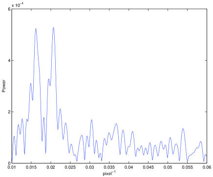
Figure 1: Stokes $V$ ripple wavelet power spectrum, obtained using the spectrum of $\alpha$ Lyr. Note the evident power at scales 0.015 - 0.022 pixel^-1 due to polarimetric ripples.

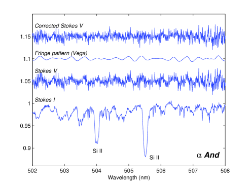
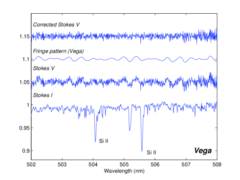
Figure 2: Ripple removal from spectra of $\alpha$ And using Vega as a template. Lower frame – Vega Upper frame - $\alpha$ And. In both frames, raw and corrected Stokes $V$, as well as the fringe pattern, have been scaled and shifted for display purposes.

Ripple removal was performed using a wavelet transform procedure (e.g. Press at al. 1992). This method allows one to isolate and filter an aperiodic signal with a complicated interaction of the amplitude, frequency and phase variation. The signal is compared not with an infinite sinusoid (as is done in the Fourier transform) but with a finite pattern. Unlike sines and cosines, wavelet functions are localised in space. Simultaneously, like sines and cosines, wavelet functions are localised in frequency or (more precisely) characteristic scale. Hence, the wavelet transform provides the possibility to isolate the contribution of a certain scale, no matter what the complexity of the signal on that scale.

Polarisation features, if they exist in the Stokes $V$ spectrum of $\alpha$ And, have full widths similar to the period of the ripples (as the projected rotational velocity $v\sin i=52$ km s^-1). Since potential polarisation features and ripples have similar scales it is hard to separate them. However, similar ripple patterns are observed in the Stokes $V$ spectrum of another, more slowly-rotating A star, $\alpha$ Lyrae (see Fig. 1), observed by Henrichs et al. during the 2003 MuSiCoS observing run. We therefore decided to use this star as a “fringing template”. $\alpha$ Lyr is a non-magnetic star, at least at the level of about 10 G (e.g. Borra, Fletcher & Poeckert 1981), and we do not expect any polarisation features in its spectra. Even if they do exist, their frequency is about twice higher (the spectral lines are narrower) than that of the fringes, and these features as well as other high frequency components such as noise are filtered out from the ripple pattern. Ultimately, we used the ripple pattern extracted from the $\alpha$ Lyr reference spectra to correct our spectra of $\alpha$ And. As can be seen in Fig. 2, ripples are significantly suppressed (although not completely removed) from the Stokes $V$ spectra. As a result, the S/N ratio in the corresponding LSD profiles (see Sect. 4) increase by 10–15%, and obvious evidence of ripples is effectively removed.

4 Extraction of LSD profiles

Least-Squares Deconvolution (LSD; Donati et al. 1997, Wade et al. 2000a) was employed to extract high-precision mean Stokes $I$ and $V$ Zeeman signatures from the MuSICoS and ESPaDOnS spectra. For the extraction we employed a specially-designed HgMn line mask (see, e.g., Shorlin et al. 2002) calculated for an effective temperature of 14000 K (Ryabchikova et al. 1999). A total of 413 lines were used in the LSD of the MuSiCoS spectra, and 582 lines in the LSD of the ESPaDOnS spectra (in the latter, excluding lines significantly blended by telluric lines).

LSD profiles obtained within $\pm 0.05$ days of each other were averaged pixel-by-pixel, finally resulting in 18 sets of Stokes $I$ and $V$ LSD profiles (summarised in Table 3) that were employed for all of the following analysis.

A careful examination of the MuSiCoS LSD profiles shows weak, residual ripples in some of the highest-S/N Stokes $V$ profiles, identifiable by a marginal but consistently higher circularly polarised flux in the red wing of the mean line. A full wavelength is apparent, and corresponds to about 200 km s^-1, in good agreement with the ripple wavelengths observed in the reduced spectra. The ripples, with full amplitudes of $1.6\times 10^{-4}$, extend well outside the mean profile. The MuSiCoS and ESPaDOnS LSD Stokes $V$ profiles are illustrated in Fig. 3.

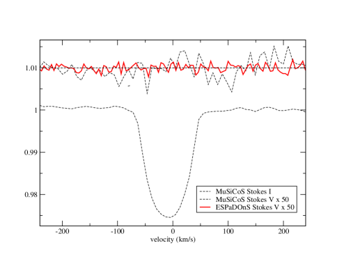
Figure 3: Example MuSiCoS (9 Jul 03) and ESPaDOnS (21 Feb 05) LSD profiles. Note the residual ripples in the MuSiCoS Stokes $V$ profile, which extend well outside the range of the Stokes $I$ profile.

#	Phase	$N_{V}$ (%)	$B_{\ell}\pm\sigma_{B}$	$|z_{V}|$	$B_{\ell}\pm\sigma_{B}$	$|z_{N}|$
			$V$		$N$
1	0.238	0.012	$90\pm 76$	1.2	$-64\pm 92$	0.7
2	0.226	0.008	$17\pm 54$	0.3	$-14\pm 53$	0.3
3	0.065	0.007	$-85\pm 44$	1.9	$59\pm 44$	1.3
4	0.419	0.008	$21\pm 53$	0.4	$-38\pm 53$	0.7
5	0.685	0.010	$-33\pm 64$	0.5	$-13\pm 63$	0.2
6	0.522	0.004	$-56\pm 29$	2.0	$-35\pm 28$	1.3
7	0.946	0.005	$-70\pm 34$	2.1	$28\pm 34$	0.8
8	0.362	0.009	$-72\pm 58$	1.3	$21\pm 57$	0.4
9	0.760	0.008	$-34\pm 52$	0.7	$-87\pm 51$	1.7
10	0.863	0.005	$-89\pm 31$	2.9	$-11\pm 30$	0.4
11	0.283	0.006	$-62\pm 39$	1.6	$35\pm 38$	0.9
12	0.699	0.005	$-59\pm 33$	1.8	$36\pm 32$	1.1
13	0.658	0.005	$-62\pm 34$	1.8	$3\pm 33$	0.1
14	0.459	0.0013	$+2\pm 8$	0.3	$+5\pm 8$	0.6
15	0.315	0.0033	$-9\pm 19$	0.5	$-30\pm 19$	1.6
16	0.404	0.0010	$-2\pm 6$	0.3	$1\pm 6$	0.2
17	0.808	0.0010	$2\pm 6$	0.3	$-3\pm 6$	0.5
18	0.240	0.0010	$-4\pm 6$	0.7	$7\pm 6$	1.2

Table 3: Final averaged LSD Stokes $I$ and $V$ profile sets and their corresponding inferred longitudinal magnetic fields. Profiles 1-13 correspond to MuSiCoS spectra; profiles 14-18 corresponds to ESPaDOnS spectra. Phases correspond to the time of mid-observations, and are calculated according to the ephemeris described in the text. $N_{V}$ is the noise level in the Stokes $V$ profile. Longitudinal fields are measured from both the Stokes $V$ and diagnostic null spectra $N$, and are reported (along with their associated detection significance $z$) in the final 4 columns.

5 Constraints on the photospheric magnetic field

5.1 Longitudinal magnetic field measurements

5.1.1 MuSiCoS and ESPaDOnS LSD profiles

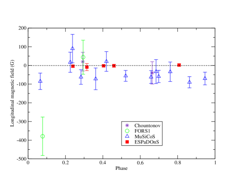
Figure 4: Longitudinal magnetic field measurements (epoch 3) as a function of rotational phase.

Longitudinal magnetic fields were inferred from each of the Stokes $I$ and $V$ profile sets, using the first-order moment method. According to this method, the longitudinal field $B_{\ell}$ (in gauss) is calculated from the Stokes $I$ and $V$ profiles in velocity units as:

$$B_{\ell}=-2.14\times 10^{12}\frac{\int vV(v)dv}{\lambda zc\int[I_{c}-I(v)]dv},$$ (1)

(Donati et al. 1997; Wade et al. 2000b) where $\lambda$, in Å, is the mean wavelength of the LSD profile, $c$ is the velocity of light (in the same units as $v$), and $z$ is the mean value of the Landé factors of all lines used to construct the LSD profile. The accuracy of this technique for determining high-precision longitudinal field measurements has been clearly demonstrated by Wade et al. (2000b), Donati et al. (2001) and Shorlin et al. (2002).

The resultant MuSiCoS longitudinal magnetic field measurements have associated 1$\sigma$ uncertainties from 29-76 G, and a median uncertainty of 44 G. Although we detect no significant longitudinal magnetic field variation, the majority of the measurements are negative, typically falling 1-2$\sigma$ below zero, with a mean of $-38\pm 12$ G. No similar bias is observed in the longitudinal field measurements inferred using the LSD diagnostic $N$ profiles.

The new LSD $B_{\ell}$ measurements are listed in Table 3.

5.1.2 FORS1 spectra

Longitudinal magnetic fields were inferred from the two FORS1 spectra of $\alpha$ And using full-spectrum regression according to the expression:

$$\Bigl{(}\frac{V}{I}\Bigr{)}=-g_{\mathrm{eff}}\ \Delta\lambda_{z}\ \lambda_{0}^{2}\ \frac{1}{I}\ \Bigl{(}\frac{{\partial}I}{\partial\lambda}\Bigl{)}\ B_{\ell}$$ (2)

(Bagnulo et al. 2002, 2005). Here, $g_{\mathrm{eff}}$ is the Landé factor (equal to 1.0 for Balmer lines, and assumed equal to 1.25 for metal lines), $\Delta\lambda_{z}$ is the Lorentz unit, $\lambda_{0}$ is the line wavelength, $I$ is observed flux at wavelength $\lambda$, and $B_{\ell}$ is the longitudinal magnetic field. As described by Bagnulo et al. (2002), the longitudinal field is obtained by a Least-Squares straight-line fit to the regression of $V/I$ versus $-\Delta\lambda_{z}\ \lambda^{2}$ (1/$I$) ($\partial I$/$\partial\lambda$). The inferred values of $B_{\ell}$, obtained using the entire spectrum (metal + Balmer lines), are reported in Table 4. Notably, one of the FORS1 measurements corresponds to a 3.7$\sigma$ detection ($B_{\ell}=-379\pm 103$ G).

HJD	Phase	$B_{\ell}\pm\sigma_{B}$ (G)
2452910.592	0.07823	$-379\pm 103$
2452963.520	0.29486	$+44\pm 91$

Table 4: Longitudinal magnetic field of $\alpha$ And inferred from FORS1 measurements.

5.2 Modeling the phased $B_{\ell}$ measurements

Of the 33 longitudinal field measurements, the best uncertainty (1$\sigma$) corresponds to three of the ESPaDOnS measurement ($6$ G), whereas the worst uncertainty corresponds to one of the measurements of Glagolevski et al. (1985; $-52\pm 118$ G), a range of almost a factor of 20 in precision! The median uncertainty of the measurements is 45 G.

The longitudinal field measurements span a total time of about $10^{4}$ days. Unfortunately, the $\pm 0.00011$ d uncertainty associated with the rotational period of Adelman et al. (2002) produces a phase uncertainty of the oldest measurements relative to the newest measurements equal to $\pm 0.19$ cycles.

All 33 $B_{\ell}$ measurements (previously published, LSD and FORS1) have been assigned phases according to the rotational ephemeris of Adelman et al. (2002):

$${\rm JD}=2449279.6898+(2.38236\pm 0.00011)\cdot E.$$ (3)

However, as indicated above, the relative phases of $\alpha$ And at the various epochs of observation are uncertain by up to $0.19\times 2\approx 0.4$ cycles. The newer and older longitudinal field data therefore cannot be phased together, and must be analysed separately.

As a first step to constrain the presence of magnetic fields in the photosphere of $\alpha$ And, we have modelled the phased longitudinal field measurements at three epochs: epoch 1 (HJD 2443383-2443388, measurements of Borra & Landstreet 1980, internal phase uncertainty of $1\times 10^{-4}$ cycles), epoch 2 (HJD 2445244-2445690, measurements of Glagolevski et al. 1985, internal phase uncertainty of $\pm 0.008$ cycles), and epoch 3 (HJD 2451798-2453423, measurements of Chountonov (2001), as well as the MuSiCoS, FORS1 and ESPaDOnS measurements reported in this paper, internal phase uncertainty of $\pm 0.03$ cycles). The phased epoch 3 measurements are illustrated in Fig. 4.

We begin by performing least-squares fits to the data. We find that the variable-field hypothesis (first-order sine fit, fitting zero-point, amplitude and phase), constant-field hypothesis (i.e. a straight line through the weighted mean), null-field hypothesis (i.e. a straight line through $B_{\ell}=0$) are indistinguishable (at the 99% confidence level) for each of the 3 epochs. We therefore conclude that no magnetic field is detected in the longitudinal field measurements of $\alpha$ And.

To quantify the magnetic field upper limit implied by the measurements, we used a modified version of the programme Fldcurv to calculate model longitudinal field variations corresponding to a large number of dipolar magnetic field configurations, varying the dipole (polar) intensity $B_{\rm p}$ as well as the obliquity angle $\beta$ and the phase of meridian crossing of the positive magnetic pole $\phi_{0}$ (which corresponds to the phase of peak positive longitudinal field). Fldcurv computes the surface distribution of magnetic field corresponding to a particular magnetic geometry, then weights and integrates the longitudinal component over the hemisphere of the star visible at a given phase. This procedure is repeated for a series of phases, producing a synthetic longitudinal field variation corresponding to the model geometry. For this procedure we have assumed a limb-darkening coefficient of 0.4.

For each model (corresponding to a grid computed with 10 G, $1\degr$ and $0.05$ sampling of $B_{\rm d},\beta$ and $\phi_{0}$, respectively) the reduced $\chi^{2}$ of the model fit to the epoch 3 observations was calculated (we select the epoch 3 observations because they will provide the best constraint, due to the ultra-high precision ESPaDOnS data). This analysis indicates that for a rotational axis inclination $i=74\pm 10\degr$ (Ryabchikova et al. 1999), acceptable magnetic models (again, at the 99% confidence level for epoch 3) are characterised by $|B_{\rm p}|<225$ G. Both $\beta$ and the phase of peak longitudinal field $\phi_{0}$ are not constrained at this confidence level (i.e. $\beta$ and $\phi_{0}$ are formally free to adopt any value between 0 and $180\degr$, and 0.0 and 1.0, respectively). Results for epochs 1 and 2 provide qualitatively similar results, with larger upper limits due to the lower precision of their respective measurements.

5.3 Modeling the phased Stokes $V$ profiles

To more robustly search for photospheric magnetic fields, we have also modelled the LSD mean Stokes $V$ profiles. To begin, we find that no Stokes $V$ signatures are detected within the boundaries of any of the 18 final individual LSD line profiles (according to the detection criterion described by Donati et al. 1997). Several of the highest-S/N MuSiCoS profiles show residual ripples which, as mentioned earlier, extend well beyond the profile boundaries.

We have calculated synthetic Stokes $I$ and $V$ LSD profiles, using the polarised line synthesis code Zeeman2 (Landstreet 1988, Wade et al. 2001), assuming a triplet Zeeman pattern and the mean Landé factor and wavelength appropriate to the $\alpha$ And line mask (the accuracy of such a modelling procedure has been demonstrated by e.g. Donati et al. 2001, 2002). Using this line model, the phase-independent LSD Stokes $I$ profile was fit, varying the line depth, projected rotational velocity and radial velocity. We then performed calculations of Stokes $V$ signatures for a large grid of dipolar magnetic field models, and compared the Stokes $V$ profile rotational variation predicted by each model with the observed LSD Stokes $V$ phase variation. The model grid was computed with sampling of 25 G, $5\degr$ and $0.05$ cycle sampling of $B_{\rm d},\beta$ and $\phi_{0}$, respectively)

We have performed independent analyses of the MuSiCoS and ESPaDOnS profiles. The results are derived from examination of concordance maps, examples of which are shown in Fig. 5. The concordance maps show the summed reduced $\chi^{2}$ for each model/data comparison as a function of the model magnetic field polar strength $B_{\rm p}$ and obliquity $\beta$. White regions correspond to models which are inconsistent with the observations at more than 99% confidence, whereas dark regions correspond to models that agree with the observations.

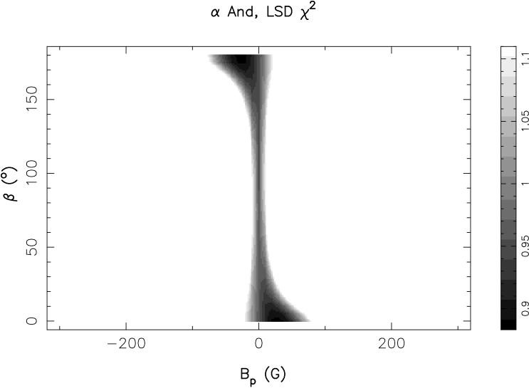
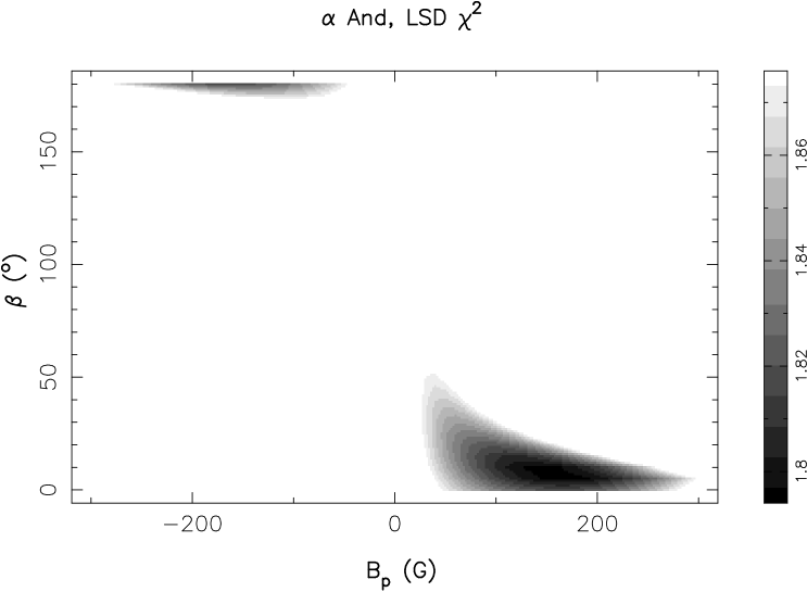
Figure 5: Reduced $\chi^{2}$ of the Stokes $V$ model/data comparison for dipole fields, as a function of the polar field strength $B_{\rm p}$ and the obliquity between the rotational axis and the magnetic field symmetry axis $\beta$. A rotational axis inclination of $i=74^{\rm o}$ has been assumed for all models. Dark regions correspond to models consistent with the observations, while white regions correspond to models incompatible with the observations at more than 99% confidence. Upper frame - ESPaDOnS data ($\phi_{0}=0.00$)  Lower frame - MuSiCoS data ($\phi_{0}=0.00$).

For the ESPaDOnS data (upper panel of Fig. 5), allowing the three parameters to vary freely, we obtain (at 99% confidence) that $|B_{\rm p}|<90$ G. Moreover, for all significantly oblique dipolar magnetic field geometries ($30\degr<\beta<150\degr$), we obtain a substantially stronger constraint: $|B_{\rm p}|<40$ G. For the ESPaDOnS profiles, both $\beta$ and $\phi_{0}$ are unconstrained, and can adopt any value between $0-180\degr$ and $0.0-1.0$, respectively.

For the MuSiCoS profiles (lower panel of Fig. 5), the results are very different. We obtain 99% confidence intervals of $|B_{\rm p}|=25-300$ G, $\beta=0-70\degr$ $\phi_{0}=0.0-1.0$, and best-fit values of $|B_{\rm p}|=150$ G and $\beta=10\degr$. Using Fldcurv to model the phased MuSiCoS longitudinal field

measurements alone, we also obtain significantly non-zero values for $|B_{\rm p}|$ ($250-1100$ G), and $\beta=0-20\degr$.

Finally, we have also calculated a series of pure quadrupolar and octupolar magnetic field models, in order to test the ESPaDOnS observations’ sensitivity to more complex field configurations. For both pure quadrupolar and octupolar fields, we find that the polar field $|B_{\rm p}|<110$ G (and $<50$ G for the majority of geometries).

5.4 Interpretation of the magnetic field results

The analysis carried out in Sect. 5.3 indicates that the combined magnetic data provide no evidence for the presence of magnetic fields in the atmosphere of $\alpha$ And. Moreover, the ultra-high precision ESPaDOnS measurements constrain any low-order multipolar magnetic field to be weaker than about 100 G.

Nevertheless, both the MuSiCoS data and one of the FORS1 measurements are not fully consistent with the general conclusion of the absence of a magnetic field. As discussed in Sect. 5.1.1, the MuSiCoS longitudinal field measurements show marginally but systematically negative values, and modelling of these data and the associated LSD Stokes $V$ profiles suggests the presence of a weak magnetic field (150 G) nearly aligned with the rotational axis of the star ($\beta=10\degr$). Such a magnetic field geometry is characterised by Stokes $V$ signatures of constant sign, and nearly constant shape and intensity. However, we have also identified residual ripples in the MuSiCoS LSD profiles. Because the residual ripples are also of constant sign and approximately constant shape and intensity, it seems rather likely that the model is fitting the residuals rather

than any real circular polarisation. This is confirmed by a detailed examination of the highest-S/N data and the best-fit model, which reveals a close correspondence between the ripple residuals and the predicted Stokes $V$ signatures. Thus we conclude with confidence that the apparent detection of a field from the MuSiCoS measurements results directly from incomplete suppression of interference ripples.

Although none of the individual MuSiCoS longitudinal field measurements corresponded to a significant detection, one of the FORS1 measurements corresponds to a field detected at 3.7$\sigma$. In order to evaluate the reliability of this marginal detection, we have performed a detailed re-analysis of the spectrum, including an examination of the contribution of individual frames and spectral regions (e.g. Bagnulo et al. 2005). First, we find no significant magnetic field in the metallic line spectrum (i.e. excluding the Balmer lines from the analysis: $B_{\ell}=-485\pm 210$ G), although with a relatively large uncertainty. Secondly, we find that all frames contribute more or less equally to the detection, and there is no indication that a particular subset of the frames is responsible for the detection. Finally, an examination of the longitudinal fields inferred from individual Balmer lines shows a diversity of results. None of the individual Balmer lines shows a significant field detection, although the combined analysis of Balmer lines with indices larger than H9 does produce a marginally significant ($3.3\sigma$) field ( notably at the level of nearly 1 kG). Most of the individual Balmer lines do show systematically negative values of the longitudinal field.

Based on this analysis alone, there is no reason to reject the apparent FORS1 detection. However, it is curious that other independent longitudinal field measurements, obtained at phases close to that of the FORS1 detection, are consistent with zero field (e.g. $-85\pm 44$ G at phase 0.065; see Fig. 4). One explanation for the apparent detection may be related to the very short exposure duration required to observe $\alpha$ And with FORS1, which is comparable to the time required to open the shutter. So, although we are unable to confidently explain the single FORS1 detection, this measurement should be interpreted in the context of the full data set (in particular as, even in the absence of a magnetic field, gaussian statistics indicates the probability of a single detection between 3 and 4$\sigma$ in a sample of 33 measurements to be 9%).

The potential for spurious detection of fields, in particular due to ripples in MuSiCoS Stokes $V$ spectra, deserves further comment. In the case of $\alpha$ And, ripples in the Stokes $V$ spectrum yielded a small but measurable contribution to the longitudinal field and the LSD Stokes $V$ signatures due to the very high S/N of the spectra, the relatively close correspondence between the ripple wavelength and the stellar line width, and the relatively small number of lines employed in the LSD. It is the combinations of these conditions that produces a situation where ripples could potentially affect the magnetic field diagnosis. A similar apparent contribution of ripples to the LSD Stokes $V$ profile is reported by Shorlin et al. (2002) for the hot Am star HD 89021 (S/N=910, $v\sin i=50$ km s^-1, $T_{\rm eff}\simeq 9000$ K), for which essentially the same conditions are satisfied. Fortunately, the presence of significant ripple contributions can be ruled out in most cases (and in particular in essentially all observations of magnetic Ap stars and cool stars) either by looking for small-amplitude structures in the LSD profile extending outside of the line profile which do not vary significantly with phase, or using observations of magnetic and non-magnetic standards. The absence of any known examples of such phenomena, apart from HD 89021 and $\alpha$ And, suggests that detectable ripple contributions are extremely rare (given that several hundred different stars have been observed using this instrument).

Retaining therefore our conclusion that $\alpha$ And is a non-magnetic star, what are the implications of our magnetic field upper limits? In the atmosphere of $\alpha$ And, at $\log\tau_{\rm 5000}=0.0$, the magneto-thermodynamic equipartition field strength (for which the magnetic and thermodynamic energy densities are approximately equal) is $B_{\rm eq}=\sqrt{12\pi nkT}\simeq 265$ G. This is significantly (2.7-6.5 times) larger than the (3$\sigma$) upper limits derived from modelling of the ESPaDOnS Stokes profiles for any low-order multipolar field that might be present.

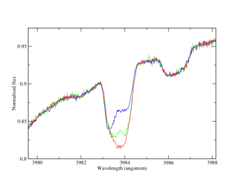
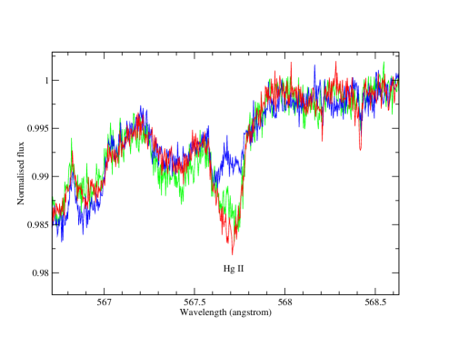
Figure 6: Variability of Hg ii 3984 and Hg ii 5677 in ESPaDOnS spectra of $\alpha$ And.

Although we have performed no quantitative modeling of more complex magnetic structures in this study (fields such as those exhibited by active late-type stars like HR 1099, e.g. Petit et al. 2004a, for example), the fact that relatively strong, complex fields are easily detected in LSD profiles of similar quality in a sample of late-type stars of similar $v\sin i$ using the MuSiCoS and ESPaDOnS spectropolarimeters strongly suggests that similar fields are not present in the photosphere of $\alpha$ And. For example, Petit et al. (2004b) find Stokes $V$ amplitudes of 0.05-0.1% due to a complex surface magnetic field in spectra of the rapidly-rotating ($v\sin i=70$ km s^-1) FK Com star HD 199178. Such signatures would be easily detectable in our LSD profiles of $\alpha$ And (either the MuSiCoS or ESPaDOnS profiles), and we can therefore rule out the presence of such complex fields as well.

Finally, although the ESPaDOnS measurements are not sufficiently sensitive to detect much weaker and/or more finely structured fields (such as those observed in the solar atmosphere), the total absence of any of the proxy phenomena well-known to be associated with such fields (spectroscopic emission lines, non-thermal radio emission, X-ray emission, flares, etc.) allows us to reasonably rule out their presence as well.

6 A search for additional line profile variability

The high quality of the MuSiCoS, ESPaDOnS and UVES spectra of $\alpha$ And makes them well-suited for a search for line profile variations similar to those reported by Adelman et al. (2002). The spectra were first searched at all locations of potential lines of Hg i, ii and iii, as predicted using the vald database (Piskunov et al. 1995). Secondly, the spectra were visually examined throughout the entire observed domain, searching for any evidence of line profile variations or unusual line shapes that might be attributed to nonuniform abundance distributions. We point out that spectral variability due to the SB2 nature of this system makes confident identification of such phenomena very challenging.

The Hg ii $\lambda 3984$ line in the UVES and ESPaDOnS spectra shows strong asymmetry and variability, and should be contrasted to nearby lines of Fe ii (Fig. 6, left panel). Thus we confirm the detection of variability in Hg ii $\lambda 3984$ as reported by Ryabchikova et al. (1999) and Adelman et al. (2002). We also observe variability of Hg ii $\lambda 6149$, $\lambda 5425$ and $\lambda 5677$. Although this variability is not confidently seen in the UVES or MuSiCoS spectra (due to lower S/N), the very high S/N ESPaDOnS spectra show the variability quite clearly (Fig. 6). In particular, the variability is evident in the spectra obtained on the successive nights from Aug 23-25 2005.

We also observe weak variability of other lines in the spectrum of $\alpha$ And. We have looked in some detail at these variations, which are present in nearly all regions of the spectra, and are quite subtle. A careful examination of the observed spectral variations on Aug 23-25 2005, in the light of synthetic spectra computed including the spectroscopic contribution of the secondary (kindly provided by T. Ryabchikova using the results of Ryabchikova et al. (1999), and taking into account the appropriate radial velocity at the time of each observation) suggests that variability of most lines can be approximately explained by the combination of spectroscopic variability due to orbital motion, small continuum normalisation differences, and weak, variable fringing. This conclusion is consistent with the observed diversity of variability characteristics of most elements (as opposed to the systematic variability observed in the Hg lines).

7 Discussion

Until recently, $\alpha$ And represented the only convincing example of a HgMn star showing intrinsic line profile variability. However, Kochukhov et al. (2005) have reported asymmetry and variability of the Hg ii $\lambda 3984$ line in spectra of two additional HgMn stars, with temperatures similar to that of $\alpha$ And. This appears to establish a new class of spotted, spectrum variable stars, of which $\alpha$ And is the prototypical example.

From our analysis of the magnetic and polarisation measurements of $\alpha$ And, we find that any oblique low-order multipolar magnetic field present in the photosphere must be weaker than about 100 G (for all field geometries), and weaker than about 50 G (for geometries with significant obliquity). Any undetected field is therefore constrained to be significantly weaker than the equipartition threshold at $\log\tau_{\rm 5000}=0.0$. If we assume that a magnetic field of at least this order is required to support horizontal abundance nonuniformities (e.g. by suppressing mixing due to meridional circulation), then an oblique low-order multipolar magnetic field does not appear to be responsible for the nonuniform distributions of Hg and Mn of $\alpha$ And, at least in atmospheric layers around $\log\tau_{\rm 5000}=0.0$. Observational support for this assumption is provided by Aurière et al. (2004), who have concluded that all magnetic Ap/Bp stars host dipolar magnetic field components that are stronger than the photospheric equipartition field (at $\log\tau_{\rm 5000}=0.0$). This supports the assumption that a field of at least this strength is required for magnetic maintenance of photospheric chemical abundance non-uniformities.

Could it be that a dipolar magnetic field does in fact exist in the photosphere of $\alpha$ And, but which is weaker than the local equipartition field in layers around $\log\tau_{\rm 5000}=0.0$? Due to the exponential decrease of the gas density with height in the outer layers of the star, such a field could in fact be stronger than the equipartition field in atmospheric layers well above (say) $\log\tau_{\rm 5000}=-1$. If the abundance non-uniformities were confined to these high layers, an undetected magnetic field (i.e. with polar intensity weaker than our 3$\sigma$ upper limit) could in principle be responsible for preventing horizontal mixing of the non-uniform abundance distributions.

The concentration of Hg, Mn and other elements in the photospheres of HgMn stars in thin layers at small optical depths has been suggested based on both theoretical and observational grounds (e.g. Proffitt et al. 1999, Sigut et al. 2000). Most recently, the discovery of emission lines in the optical spectra of some HgMn stars (e.g. Sigut et al. 2000, Wahlgren & Hubrig 2000) has provided additional evidence of stratification of these elements. Sigut (2001), interpreting the presence of Mn ii emission lines in the spectra of HD 186122 and HD 179761 as the result of interlocked non-LTE effects combined with chemical stratification, found that Mn must be confined to column masses above $\log\Sigma=-1.5$, equivalent to about $\log\tau_{\rm 5000}\mathrel{\hbox{\hbox to0.0pt{\hbox{\lower 4.0pt\hbox{$\sim$}}\hss}\hbox{$<$}}}-1.1$. Although we observe no such emission lines in the spectrum of $\alpha$ And, were Hg confined to very small optical depths in the atmosphere of this star (i.e. optical depths at which the equipartition field satisfies our field constraints - for $\alpha$ And, $B_{\rm eq}$ should be below 100 G above $\log\tau_{\rm 5000}=-1.2$, and below 50 G above $\log\tau_{\rm 5000}=-2.2$) it might be possible for an undetected magnetic field to sustain the lateral abundance non-uniformities.

In order to test this possibility, we have performed some comparisons between the observed Hg line profiles and those predicted by a single-step stratified Hg distribution, in which Hg is 100 times more abundant above $\log\tau_{\rm 5000}=-1.2$ than below, and in which the lower zone abundance (we employed $\epsilon_{\rm Hg}=-5.0$) has been chosen to approximately fit the profile of Hg ii $\lambda 3984$. Unfortunately, the combination of line asymmetry and variability, coupled with the weakness of many of the Hg lines (1-2% deep) and local continuum normalisation errors, makes it impossible to realistically choose between the stratified and unstratified models.

Ultimately, we are led to conclude that models seeking to explain the nonuniform Hg surface distribution of $\alpha$ And which invoke the presence of a magnetic field of $B\mathrel{\hbox{\hbox to0.0pt{\hbox{\lower 4.0pt\hbox{$\sim$}}\hss}\hbox{$>$}}}100$ G are almost certainly falsified by the results presented in this paper. It may still be possible to implicate a dynamically-important magnetic field if Hg is strongly stratified, and confined primarily to upper layers of the atmosphere (where the equipartition field is weaker than the upper limits presented here). Based on our experiments, modeling of the vertical Hg distribution will require very high quality data (of quality similar to or better than that discussed here), coupled with a model which simultaneously considers the lateral and vertical abundance distribution. However, in the absence of evidence of strong Hg stratification, we conclude that a non-magnetic mechanism is almost certainly responsible for this phenomenon (see e.g. Kochukhov et al. 2005).

References

- (1) Adelman S.J., 1998, A&AS 132, 93
- (2) Adelman S.J., Gulliver A.F., Kochukhov O., Ryabchikova T.A., 2002, ApJ 575, 449
- (3) Aurière M., Silvester J., Wade G.A., Bagnulo S., et al., 2004, in the proceedings of Magnetic Stars, Special Astrophysical Observatory, Yu. Glagolevski & I.I. Romanyuk (eds.), page 114
- (4) Ballester P., Grosbol P., Banse K., Disaro A., et al., 2000, SPIE 4010, 246
- (5) Bagnulo S., Szeifert T., Wade G.A., Landstreet J. D., Mathys G., 2002, A&A 389, 191
- (6) Bagnulo S., Landstreet J. D., Mason E., Andretta V., Silaj J., Wade G.A., , 2005, A&A, submitted
- (7) Baudrand J., Böhm T., 1992, A&A 259, 711
- (8) Bohlender D.A., 1988, Ph.D. thesis, University of Western Ontario
- (9) Borra E.F. & Landstreet J.D., 1980, ApJS 42, 421
- (10) Borra E.F., Fletcher J.M. & Poeckert R., 1981, ApJ 247, 569
- (11) Chountonov G., 2001, in Magnetic fields across the HR diagram, ASP conference series #248, G. Mathys, S. Solanki & W. Wickramasinghe (eds.), p. 385
- (12) Donati J.F., Semel M., Carter B.D., Rees D.E., Cameron A.C., 1997, MNRAS 291, 658
- (13) Donati J.-F., Catala C., Wade G.A., Gallou G., Delaigue G., Rabou P., 1999, A&AS 134, 149
- (14) Donati J.-F., Wade G.A., Babel J., Henrichs H.F., de Jong J.A., Harries T., 2001, MNRAS 326, 1265
- (15) Donati J.-F., Babel J., Harries T., Howarth I., et al., 2002, MNRAS 333, 55
- (16) Glagolevski Yu., Romanyuk I.I., Bychkov V.D., Najdenov I.D., 1985, PAZh, 11, 107
- (17) Johnson N.M., 2004, M.Sc. Thesis, Royal Military College of Canada
- (18) Kockhukhov O., Piskunov N., Sachkov M., Kudryavtsev D., 2005, A&A, 439, 1093
- (19) Landstreet J.D., 1988, ApJ 326, 967
- (20) Landstreet J.D. & Mathys G., 2000, A&A 359, 213
- (21) Petit P., Donati J.-F., Wade G.A., Landstreet, et al., 2004a, MNRAS 348, 1175
- (22) Petit P., Donati J.-F., Oliveira J.M., Auriìere M., et al., 2004b, MNRAS, in press
- (23) Piskunov N.E., Kupka F., Ryabchikova T.A., Weiss W.W., Jeffery C.S., 1995, A&AS 112, 525
- (24) Proffitt C., Brage T., Leckrone D., Wahlgren G., Brandt J., Sansonetti C., Reader J., Johansson S., 1999, ApJ 512, 942
- (25) Press W.H., Teukolsky S., Vetterling W., Flannery B., 1992, Numerical Recipes in C, Cambridge University Press
- (26) Ryabchikova T.A., Malanushenko V.P., Adelman, S.J., 1999, A&A 351, 963
- (27) Semel M., 2003, A&A 401, 1
- (28) Shorlin S.L.S., Wade G.A., Donati J.-F., Landstreet J.D., Petit P., Sigut T.A.A., Strasser S., 2002, A&A 392, 637
- (29) Sigut T.A.A., Landstreet J.D., Shorlin S.L.S., 2000, ApJ 530, L89
- (30) Sigut T.A.A., 2001, A&A 377, L27
- (31) Wade G.A., Donati J.-F., Landstreet J.D., Shorlin S.L.S., 2000a, MNRAS 313, 823
- (32) Wade G.A., Donati J.-F., Landstreet J.D., Shorlin S.L.S., 2000b, MNRAS 313, 851
- (33) Wade G.A., Bagnulo S., Kochukov O., Landstreet J.D., Piskunov N., Stift M.J., 2001, A&A 374, 265
- (34) Wahlgren G. & Hubrig S., 2000, A&A 362, 13