Velocity field and star formation in the Horsehead nebula

Using large scale maps in ${\rm C^{18}O}$$(2-1)$ and in the continuum at 1.2mm obtained at the IRAM-30m antenna with the Heterodyne Receiver Array (HERA) and MAMBO2, we investigated the morphology and the velocity field probed in the inner layers of the Horsehead nebula. The data reveal a non–self-gravitating ($m/m_{\rm vir}\approx 0.3$) filament of dust and gas (the “neck”, $\varnothing=0.15-0.30\,{\rm pc}$) connecting the Horsehead western ridge, a Photon-Dominated Region illuminated by $\sigma$Ori, to its parental cloud L1630. Several dense cores are embedded in the ridge and the neck. One of these cores appears particularly peaked in the 1.2 mm continuum map and corresponds to a feature seen in absorption on ISO maps around 7 $\mu$m. Its ${\rm C^{18}O}$ emission drops at the continuum peak, suggestive of molecular depletion onto cold grains. The channel maps of the Horsehead exhibit an overall north-east velocity gradient whose orientation swivels east-west, showing a somewhat more complex structure than was recently reported by Pound et al. (2003) using BIMA CO$(1-0)$ mapping. In both the neck and the western ridge, the material is rotating around an axis extending from the PDR to L1630 (angular velocity $=1.5-4.0\,{\rm km\,s^{-1}}$). Moreover, velocity gradients along the filament appear to change sign regularly (3 ${\rm km\,s^{-1}\,pc^{-1}}$, period=0.30 pc) at the locations of embedded integrated intensity peaks. The nodes of this oscillation are at the same velocity. Similar transverse cuts across the filament show a sharp variation of the angular velocity in the area of the main dense core. The data also suggest that differential rotation is occurring in parts of the filament. We present a new scenario for the formation and evolution of the nebula and discuss dense core formation inside the filament.

1 Introduction

Dense molecular cores are the basic units of isolated low-mass star formation. It is now common that molecular line mapping from dark clouds reveals clumps embedded in filamentary structures (e.g. Onishi et al., 1998, 1999; Obayashi et al., 1998; Loren, 1989a; Chini et al., 1997). These filaments can be either self-gravitating or not. The clumps are mostly gravitationally bound, and in many cases, star formation is known to have already started. Therefore, molecular filaments are thought to play a crucial role in low-mass star formation.

However, little is known about the general physical properties of these filaments. For example, the density distribution is very likely not uniform, but instead varies according to a power-law. Stepnik et al. (2003) have investigated this observationally in a filament of the Taurus molecular cloud, and concluded that a $r^{-2}$ profile was compatible with the observations. Steeper density profiles can however be observed, as is shown by Hily-Blant & Falgarone (in prep) in a non–self-gravitating filament connected to the low-mass dense core L1512. Theoretical models with and without magnetic fields suggest power-laws with exponents ranging from $\approx-2$ (Fiege & Pudritz, 2000) to $-4$ (Ostriker, 1964; Nakamura et al., 1993; Stodólkiewicz, 1963).

The importance of the velocity field in the formation of clumps in filamentary clouds has already been noted several years ago by Loren (1989b), who did a systematic study of the velocity pattern of well-known filaments in $\rho\rm Oph$. The longitudinal velocity was shown to exhibit gradients near the locations of the main clumps harboured in the filament. From the theoretical and numerical points of view, recent studies also stress the role of the velocity field. Dealing with self-similar rotating magnetized cylinders, Hennebelle (2003) shows that the velocity field strongly depends on the relative intensity of the toroidal component of the magnetic fields with respect to the poloidal one and to the gravitational force: the rotation can be mainly that of a rigid body or instead be differential. The importance of the velocity field has been further stressed by Tilley & Pudritz (2003) who show how it could help in distinguishing between collapsing and equilibrium cylindrical distributions and between magnetized and unmagnetized filaments. Fiege & Pudritz (2000) performed numerical studies of the fragmentation of pressure truncated isothermal filaments threaded by helical magnetic fields and found that the toroidal velocity could change sign periodically when magnetic field dominates over gravity. More recently, Sugimoto et al. (2004) numerically studied the decay of Alfvén waves in filamentary clouds. They show that the propagating circularly polarized waves generate longitudinal sub-waves that steepen into shocks where the initial energy is being dissipated. While propagating, the circularly polarized Alfvén waves make the filament rotate. In some cases, the filament can fragment into regularly spaced clumps.

Instabilities (gravitational, magnetic, or both) are often invoked to explain the formation of dense cores in filaments. Nonetheless, molecular observations of filamentary structures at high spatial and spectral resolution are still lacking, which would allow both the density and the velocity fields to be constrained. The scales of interest are typically of the order on 0.1 pc and velocity gradients of the order on 1 ${\rm km\,s^{-1}\,pc^{-1}}$. In this paper, we investigate the velocity field and its link to the density distribution in the Horsehead nebula, a close-by (400 pc) dark protrusion emerging from its parental cloud L1630 in the Orion B molecular complex. This condensation is illuminated by the O9.5V star $\sigma$Ori (distance 0.5^∘ from the cloud) and presents a Photon-Dominated Region (PDR) on its western side seen perfectly edge-on (Abergel et al., 2003). Until some years ago, molecular observations of this source were still scarce and limited to low spatial resolution (2^′ resolution, Kramer et al., 1996). New insights at higher resolution (10–20^′′) have recently been revealed by Abergel et al. (2003) and Pound et al. (2003), who observed the Horsehead in various millimetre transitions and isotopes of CO. In particular, Pound et al. (hereafter PRB03) analyse the velocity field of this source, using interferometric CO$(1-0)$ data (10^′′$\times$8^′′ resolution), and reported a general NE-SW velocity gradient of order 5 ${\rm km\,s^{-1}\,pc^{-1}}$ across the nebula. They also note that star formation may have already started in the cloud and discuss possible scenarios that could have driven the formation of such a structure. The use of an optically thick probe may however, have hindered them from obtaining a thorough picture of the structure in the innermost layers of this object. In the present study, we make use of the rarer isotopomer ${\rm C^{18}O}$, as well as the emission of dust at millimeter wavelengths.

The paper is organized as follows. After a brief description of the observations in Sect. 2, we analyst in Sect. 3 the spatial distribution of the ${\rm C^{18}O}$$(2-1)$ emission and of support data obtained in the continuum at various wavelengths to derive representative physical parameters. The analysis of the velocity field is then explained in Sect. 4, and its consequences on the genesis and evolution of the object are then discussed in Sect. 5. We finally summarize our conclusions in Sect. 6.

2 Observations

The ${\rm C^{18}O}$$(2-1)$ data presented in this paper have been observed in May 2003 using the new Heterodyne Receiver Array (HERA, Schuster et al., 2003, 2004) operated at the IRAM-30m telescope. The data were obtained in the On-The-Fly mode with an array inclined on the sky by 18.5^∘ in the equatorial frame, providing a direct sampling of 8^′′ in Declination, while a derotator located in the receiver cabin was used to keep the HERA pixel pattern stationary in the Nasmyth focal plane. The half-power beam-width is 12^′′. The data were obtained under good-to-average weather conditions and system temperatures were on the order of 400 K, providing an average noise r.m.s. in the regridded map of 0.2 K ($T_{\rm A}^{*}$ scale) within 0.1 ${\rm km\,s^{-1}}$ velocity channel. The final data are scaled in $T_{\rm mb,c}$, a temperature scale which takes into account the emission peaked-up by the 30-m error beam at 1.2 mm (see Abergel et al., 2003, and references therein for details). Figure 1 shows the corresponding integrated intensity map in the velocity interval $[9.1:11.8]$ ${\rm km\,s^{-1}}$.

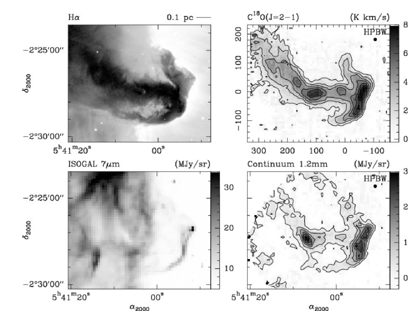
Figure 1: (Upper left): H$\alpha$ line emission map obtained at the 0.9 m KPNO telescope (courtesy of Reipurth & Bally). (Upper right): Integrated emission map ($\int T_{\rm mb,c}\mathrm{d}v$, ${\rm K\,km\,s^{-1}}$, $v\in[9.1:11.8]\,{\rm km\,s^{-1}}$) of C¹⁸O$(2-1)$. Offsets are in arcsec and contours are 1.2 to 7.2 by 1.2 ${\rm K\,km\,s^{-1}}$. The half-power beam width (HPBW) is plotted at the top right corner. (Bottom left): continuum emission around 7 $\mu$m (mostly aromatic emission) covered by ISO. (Bottom right): Continuum emission at 1.2 mm observed by MAMBO2. Contours are 0.15 MJy/sr to 2.65 MJy/sr by 0.5 MJy/sr.

As a complement, we also use continuum emission maps at 1.2 mm obtained with MAMBO2, the MPIfR 117-channel bolometer array operated at Pico Veleta (Kreysa, 1992). These data are partially shown in a companion paper (Teyssier et al., 2004), but are presented here infull for the first time. We refer to this article for further details about the observations. Also used in this analysis is the ISOCAM map obtained on this source by Abergel et al. (2002, 2003) in the LW2 filter (5.-8.5 $\mu$m). The corresponding maps are displayed in Fig. 1, in combination with the H$\alpha$ coverage obtained by Reipurth & Bally (private communication) at the KPNO 0.9 m telescope.

3 Morphology

3.1 Spatial distribution

Observation of an optically thin species provides a detailed picture of the inner molecular layers of this complex object for the first time. The spatial distribution correlates remarkably well with the visible dust absorption (well represented here by the H$\alpha$ image) and the optically thin dust continuum emission at 1.2 mm, revealing a somewhat different shape than the Horsehead silhouette as traced e.g. by the BIMA CO$(1-0)$ maps of PRB03 (10^′′$\times$8^′′resolution). Also, the ${\rm C^{18}O}$ map presented here extends further east than the ${\rm{}^{12}CO}$ map of these authors. In particular, the western ridge forming the PDR appears connected to the parental cloud through a thin (1.5^′, or 0.2 pc at a distance of 400 pc) dust and gas east-west filament (hereafter called the “neck”) exhibiting three noticeable integrated intensity peaks. This filament penetrates further inside the L1630 cloud following a SW-NE orientation. In this study, we distinguish between these two sections of the neck and refer to the “inner” (eastmost) and “outer” (westmost) necks, respectively. Similarly, we refer to the northern part of the PDR as the “nose” and to its southern part as the “mane”, following some of the naming already used by PRB03. The material voids present north and south of the outer neck will be respectively called the jaw and the optical hole. These areas are indicated in Fig. 5. We note that our ${\rm C^{18}O}$$(2-1)$ integrated intensity map is much less clumpy than that in ${\rm{}^{12}CO}$$(1-0)$ from PRB03, particularly in the outer neck. Since ${\rm{}^{12}CO}$$(1-0)$ traces the lower density material, this suggests that the external envelope is clumpier than the inner parts evidenced by the ${\rm C^{18}O}$$(2-1)$. Indeed some ${\rm{}^{12}CO}$$(1-0)$ peaks of integrated intensity (e.g. in the mane) do match optical features, with no counterpart in ${\rm C^{18}O}$$(2-1)$. However, it is not clear whether this is due to excitation or photo-dissociation selective effects, or to a combination of both.

A noticeable emission peak is observed at the base of the pillar formed by the outer neck (hereafter Peak2, $\alpha_{2000}$=05^h41^m06^s, $\delta_{2000}=-2$^∘27^′30^′′), which coincides with an embedded structure seen in absorption at 7 and 15 $\mu$m (Abergel et al., 2002, see also Fig. 1) and a strong emission feature in the continuum at 1.2 mm, also prominent in other submm continuum maps obtained by SCUBA at the JCMT (850 and 450 $\mu$m, Sandell private communication) and SHARC-II at the CSO (350 $\mu$m, Lis private communication). It is interesting to note that the position of the peak associated with this clump differs in the 1.2mm continuum and in the ${\rm C^{18}O}$$(2-1)$ maps, a phenomenon often associated with molecular depletion onto grains (e.g. Caselli et al., 1999) and indicative of high densities and cold temperatures. In the ${\rm{}^{12}CO}$$(1-0)$ map from PRB03, an elongated maximum is seen north of Peak2 position, but it does not coincide with either of our ${\rm C^{18}O}$$(2-1)$ or continuum maxima in this area. A detailed study of this condensation is, however, beyond the scope of the present paper and will be addressed in a forthcoming work (Teyssier & Hily-Blant, in preparation). Three other peaks are seen in the neck: Peak1 ($\alpha_{2000}$=05^h40^m59^s, $\delta_{2000}=-02$^∘27^′18.7^′′), Peak3 (($\alpha_{2000}$=05^h41^m12.2^s, $\delta_{2000}=-02$^∘25^′59^′′), and Peak4 ($\alpha_{2000}$=05^h41^m15.3^s, $\delta_{2000}=-02$^∘25^′39.5^′′, see also Fig. 5). We note that Peak1 has counterparts in the 1.2mm continuum map; however, it does not stand out at all in the interferometric map of PRB03. On the other hand, Peak3 and Peak4 are only visible in the molecular data, and in limited velocity ranges, $[9.9:10.1]$ and $[10.3:10.6]$ ${\rm km\,s^{-1}}$ respectively (see Fig. 2).

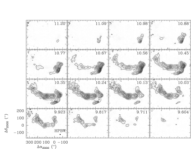
Figure 2: Channel maps of the C¹⁸O$(2-1)$ emission between 9.6 and 11.2 ${\rm km\,s^{-1}}$. Contours are 1.1 K to 7.4 K by steps of 0.9 K ($T_{{\rm A}}^{*}$ scale, rms=0.2 K).

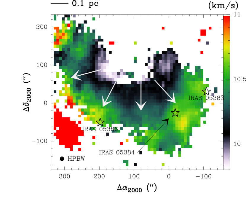
Figure 3: Map of the C¹⁸O$(2-1)$ velocity centroids. Indicated by stars are three IRAS sources identified by Sandell et al. (1986). The arrows indicate the velocity gradient orientations at different positions across the neck and ridge.

Figure 4: Map of ${\rm C^{18}O}$$(2-1)$ spectra averaged over areas of 40^′′$\times$40^′′. The vertical dotted line indicates the systemic velocity (10.33${\rm km\,s^{-1}}$). The channel width is 0.1 ${\rm km\,s^{-1}}$. Offsets are in (^′′).

3.2 Physical conditions

This section is not meant to study the variation of the physical parameters at small scale in detail but rather to give an overview of the typical conditions associated to the areas introduced above. This analysis has already been conducted in the PDR by Abergel et al. (2003) and Teyssier et al. (2004), who report peak visual extinctions in the range 12-25 mag and densities on the order of 2$\times 10^{4}$${\rm cm^{-3}}$. However, based on high resolution ${\rm H_{2}}$ NIR data, Habart et al. (2003, see also ) have shown that this last parameter could be higher by one order of magnitude at the PDR border. At the scales of interest, we used the 1.2mm continuum emission in order to compute the column densities. We applied the formula presented in Motte et al. (1998), assuming dust temperatures of 35 K in the PDR area (Teyssier et al., 2004) and of 10 K for all areas eastward of the ridge. The dust mass opacity at 1.2mm is known to vary depending on the temperature and/or density (e.g. Ossenkopf & Henning, 1994; Stepnik et al., 2003). To account for this uncertainty, we considered values of this parameter in the range 3–6$\times 10^{-3}$ g ${\rm cm^{-2}}$. Excluding the 3 peaks introduced above, the computed column densities vary between some ${\rm 10^{21}}$ ${\rm cm^{-2}}$ in the most diffuse parts (distributed over the inner and outer necks) and 1.0–2.5$\times 10^{22}$ ${\rm cm^{-2}}$ (e.g. in the mane or the PDR). While Peak1 and Peak3 exhibit quantities in the range of those in the PDR, the Peak2 column density is calculated to be 3.5$\pm$1.0$\times 10^{22}$ ${\rm cm^{-2}}$.

In order to compare these estimates with quantities derived from the molecular tracers, we used complementary observations of CO$(2-1)$ (Güsten, private communication) and ${\rm C^{18}O}$$(1-0)$ (Teyssier, private communication) at positions of interest to run LVG simulations. Assuming optically thick emission from CO$(1-0)$, we inferred lower limits to the kinetic temperature to be applied to ${\rm C^{18}O}$. $T_{{\rm kin}}$ are found in the range 20-30 K, translating into volume densities of ${\rm 10^{4}}$ ${\rm cm^{-3}}$ in most of the ridge and outer neck. Somewhat lower values (factor 2-3 below) are found in the inner neck, while Peak2 exhibits a higher density of $n_{\rm H_{2}}$=4$\times 10^{4}$ ${\rm cm^{-3}}$. The ${\rm C^{18}O}$ column density was simultaneously constrained and translated into ${\rm H_{2}}$ column densities using the calibration described in Teyssier et al. (2004): $N_{{\rm H_{2}}}=(2.5\pm 0.6\times 10^{6})\,\times\,N({\rm C^{18}O})+1.4\times 10^{21}\,{\rm cm^{-2}}$. $N_{{\rm H_{2}}}$ is found to be in very good agreement with the estimates based on the dust emission, except at the position of Peak2 where a value of 1.4$\times 10^{22}$ ${\rm cm^{-2}}$ is measured, suggestive again of molecular depletion in the cold condensation. We estimate from this that the quantities derived in this core from ${\rm C^{18}O}$$(2-1)$ are under-estimated by a factor of at most 3. Table LABEL:tab:_phys_condition compiles these values for various areas of interest.

Table 1: Physical conditions in the Horsehead (see Sect. 3.2).
^(a) corrected from molecular depletion, ^(b) from Abergel et al. (2003).

	diffuse parts	Peak2(a)	PDR(b)
$n_{{\rm{\rm H_{2}}}}$ (${\rm cm^{-3}}$)	3–5$\times 10^{3}$	4$\times 10^{4}$	2$\times 10^{4}$
$N_{{\rm H_{2}}}$ (${\rm cm^{-2}}$)	$\approx$1021	$3.5\pm 1.0$$\times 10^{22}$	1.2–2.5$\times 10^{22}$

We finally compared the values of $N_{{\rm H_{2}}}$ and n${}_{\rm H_{2}}$ to infer the cloud depth along the line of sight. Their ratio indicate depths in the range 0.15–0.30 pc, very similar to the filament width on the sky. Within the effects of projection, this is consistent with a more or less cylindrical shape of the filament.

3.3 Mass estimates

With these numbers, we estimated the overall mass of the material traced by ${\rm C^{18}O}$$(2-1)$. The analysis presented above shows that $H_{2}$ column density estimates based on either our 1.2mm dust continuum or the ${\rm C^{18}O}$$(2-1)$ integrated intensity maps are in good agreement provided molecular depletion onto grains is not a concern. This assumption is fairly justified here, with the exception of the dense core associated to Peak2. Assuming an overall conversion factor of $N_{{\rm H_{2}}}/W({\rm C^{18}O(2-1)})=2.5\times 10^{21}$ ${\rm cm^{-2}}$/(${\rm K\,km\,s^{-1}}$), the total mass derived from the ${\rm C^{18}O}$$(2-1)$ integrated intensity is found to be 19 M_⊙, of which 0.6 $\rm M_{\odot}$are located in the cold core. Assuming a depletion factor on the order of 3 (see previous section) in the Peak2 area, the total corrected mass amounts to 20 $\rm M_{\odot}$, showing that depletion effects are negligible as regards the total area considered. This is lower by 25% than the value reported by PRB03, and very likely does not account for all the material present in the nebula, since here we are probing only the gas in the inner layers.

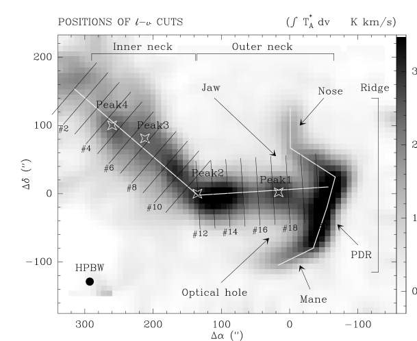
Figure 5: Position of the position-velocity cuts drawn over the integrated emission map of C¹⁸O$(2-1)$. The full lines correspond to the cuts across the neck and ridge, respectively, while the thin black lines illustrate the position of the radial cuts, spaced by 22 ^′′($\approx 2$ HPBW), with some numbers referring to the cuts shown in Fig. 9. The crosses indicate the position of the four peaks introduced in Sect. 3.1. Also indicated are the areas discussed throughout this paper.

4 Study of the velocity field

In this section, we present the detailed analysis of the velocity field based on the ${\rm C^{18}O}$$(2-1)$ data. The systemic velocity as deduced from the integrated spectra over the whole field is $v_{0}$=10.33 ${\rm km\,s^{-1}}$. The shape is very nearly Gaussian with a total FWHM of 0.8 ${\rm km\,s^{-1}}$. This value falls in between typical linewidth in dark clouds (nearly thermal, 0.5 ${\rm km\,s^{-1}}$) and that of the more diffuse molecular phase (1 ${\rm km\,s^{-1}}$). This in fact reflects the wide range of velocities in the nebula where the overall linewidth is broadened by velocity gradients. Individual spectra indeed have FWHM=0.66$\pm$0.11${\rm km\,s^{-1}}$, as illustrated in Fig. 4 where averaged spectra over small areas are plotted. While the centroid velocity changes within the nebula, the lineshape remains Gaussian.

Another picture of this effect is shown in the line centroid map displayed in Fig. 3. The computation was done in such a way that the spectral window used to deduce the centroid is optimized for each spectrum. This method is described in Pety & Falgarone (2003), and consists in maximizing the signal-to-noise ratio on the integrated area in the actual spectral window. The centroid is then computed in the usual way, i.e. as the velocity weighted by the temperature. As was already reported by PRB03, the map in Fig. 3 reveals an overall North (blue-shifted emission)–South (red-shifted emission) velocity gradient of about 4-5 ${\rm km\,s^{-1}\,pc^{-1}}$. However, this gradient has a somewhat more complex morphology, as its orientation seems orthogonal to a parabolic-like curve starting (at least within our map boundaries) from the inner neck basis and slowly folding towards the Horse’s nose. The gradient orientation is thus swivelling east-west, as indicated by the arrows drawn on Fig. 3. The NE-SW gradient mentioned by PRB03 thus only applies to the western part of the dark protrusion. The data also indicate that both red and blue velocity components seem to be wrapped around an axis coincident with the neck shape. It is interesting to note the coincidence between the peaks in velocity centroids (around 10.8 ${\rm km\,s^{-1}}$) and the locations of three of the IRAS stars identified in the field (Fig. 3). A similar phenomenon could already be seen on the map of PRB03. We do not, however, see any obvious explanation for this effect.

The channel map displayed in Fig. 2 shows the structures associated to the ${\rm C^{18}O}$$(2-1)$ velocity field. The ridge and the neck appear clumpy, with the intensity peaks moving when going from one velocity channel to the other. This is indicative of a rich velocity field inside the structure. In order to identify the mechanisms associated to this gas motion, we study position-velocity maps performed along various dedicated cuts in the following sections.

4.1 Longitudinal cuts

We first consider cuts performed along the filamentary structures introduced in Sect. 3.1. The positions of these two cuts (respectively along the neck and the western ridge) are displayed in Fig. 5. Although there is some subjectivity in the choice of these segments, we followed, as much as possible, the morphology traced by the filamentary structures in the integrated intensity map.

Figure 6 displays the first of these cuts computed along the western ridge, showing a large north-south velocity gradient extending over more than 0.4 pc. The relatively linear slope of this gradient (on the order of +2.6 ${\rm km\,s^{-1}\,pc^{-1}}$) suggests that the material is rotating. The PDR and nose thus seem to be wrapped around an axis coincident with the outer neck. Further along the cut, the velocities associated to the gas traced in the mane experience a fast drop with a gradient of $-4.3$ ${\rm km\,s^{-1}\,pc^{-1}}$. The mane thus appears to be braked back to the systemic velocity found in the filament. We discuss in Sect. 5 an interpretation of this peculiar behaviour.

The respective $l-v$ map in the neck is shown in Fig. 7. In the gas associated to the outer neck, departures from the systemic velocity are less pronounced than in the ridge. However a close look at the inner neck indicates that the velocity gradient appears to change sign regularly (amplitude of approximately 2.5 ${\rm km\,s^{-1}\,pc^{-1}}$, rough period of 2.5^′, or 0.3 pc). The nodes of this modulation are found at a common velocity of 10.2 ${\rm km\,s^{-1}}$(see Fig. 7). It is interesting to note that Peaks 3–4 are located where the velocity gradient changes sign. This gradient then experiences another rapid flip as one penetrates the L1630 cloud (new value of –4.8 ${\rm km\,s^{-1}\,pc^{-1}}$) further.

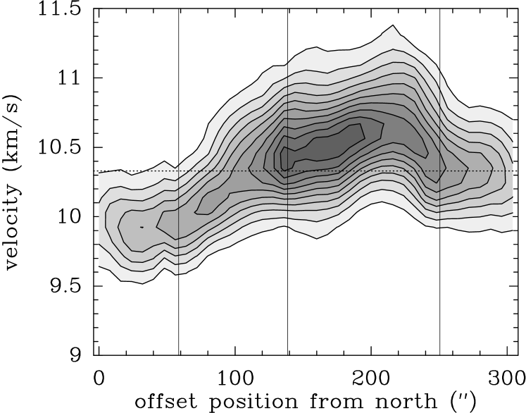
Figure 6: ${\rm C^{18}O}$$(2-1)$ position-velocity cut performed along the western ridge and the mane (from north to south, Fig. 5). The dashed horizontal line indicates the systemic velocity $v_{0}$. The three vertical lines delineate the four segments forming the cut. A large (+2.6 ${\rm km\,s^{-1}\,pc^{-1}}$) north–south velocity gradient is observed until the mane, where the gradient is suddenly inverted to finally end up at the systemic velocity with a slope of –4.3 ${\rm km\,s^{-1}\,pc^{-1}}$. Contours start at 3$\sigma$ (0.6 K), in steps of 3$\sigma$.

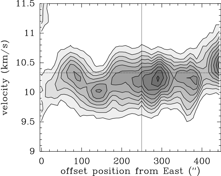
Figure 7: Same as Fig. 6 along the entire neck (from east to west, Fig. 5). The dashed line indicates the systemic velocity, while the vertical one shows the position of Peak2 (see Sect. 3.1), where the longitudinal cut changes direction. Positions of peaks 4 to 1 are at offsets 80, 140, 250 and 380 ^′′ respectively. Recall that Peak2 is not a maximum in the ${\rm C^{18}O}$$(2-1)$ integrated intensity map and was inferred from the continuum data. Note the 3 different velocity gradients (positive, negative, positive) as one moves from 0 to 200 ^′′(see text for details). Contours start at 3$\sigma$ (0.6 K), in steps of 3$\sigma$.

4.2 Radial cuts

Radial cuts across the neck allow a probe of the gas motion around the axis defined by the filament projected shape. To this aim, we have constructed $l-v$ maps on a series of small slits perpendicular to the neck longitudinal cut analyzed previously. Their positions and associated numbers are indicated in Fig. 5. The corresponding collection of maps is gathered in Fig. 8. In most cases, the velocity scales almost linearly with the radial position, again indicative of rigid body rotation and confirming that the neck itself is spinning around its own axis. However, some cuts (e.g. #6, #7, #11, #12) depart from that linear behaviour, suggesting that differential rotation may affect the transverse gas motion in these areas. Such velocity gradients across the neck could also result from a velocity shear perpendicular to the neck. This interpretation will be compared to rotation in Sect.5.2.

It is also interesting to note that the velocity gradient observed at each position is varying when moving from east to west. In order to quantify this variation, and motivated by the assumption of rigid body rotation, we performed a systematic linear fit of each individual $l-v$ cut and interpreted this slope of as an angular velocity. In each cut, spectral lines were fitted by Gaussians, and their central velocity was stored. This set of central velocities was then weighted taking into account both the signal-to-noise ratio (SNR) of the data and the error on the centroid itself, and finally fitted by a linear slope. The result of this computation is illustrated in Fig. 9, where gradients are plotted against the distance along the neck. The resulting plot reveals a striking shape: while the outer neck appears in rigid body rotation at 1.5 ${\rm km\,s^{-1}\,pc^{-1}}$ (corresponding to a rotation period of 4 Myrs, roughly equal to the survival time of the Horsehead, 5 Myrs, estimated by PRB03), parts of the inner neck experience a sharp increase in velocity gradient when moving from east to west (from 1.5 to 4 ${\rm km\,s^{-1}\,pc^{-1}}$ in about than 0.1 pc). This rapid jump is followed by a similar decrease back to the 1.5 ${\rm km\,s^{-1}\,pc^{-1}}$ velocity gradient. Beyond this point, the radial cuts associated to the westmost part of the inner neck are found to have a 0 velocity gradient (within the slope fit uncertainty). It is to be noted that all three positions of Peaks 1, 2, and 4 are found at the common velocity gradient of 1.5 ${\rm km\,s^{-1}\,pc^{-1}}$ (it is less true for Peak1, though), while Peak3 is found at the high velocity gradient of 4 ${\rm km\,s^{-1}\,pc^{-1}}$. Interestingly enough, Peak3 sits almost in the middle of the roughly symmetric gradient increase bracketed by Peaks 2 and 4. At the eastmost offsets, the radial cuts exhibit another gradient increase, but this one is very likely due to the known large gradient found along the mane and nose, and is less meaningful in terms of radial gradient across the neck.

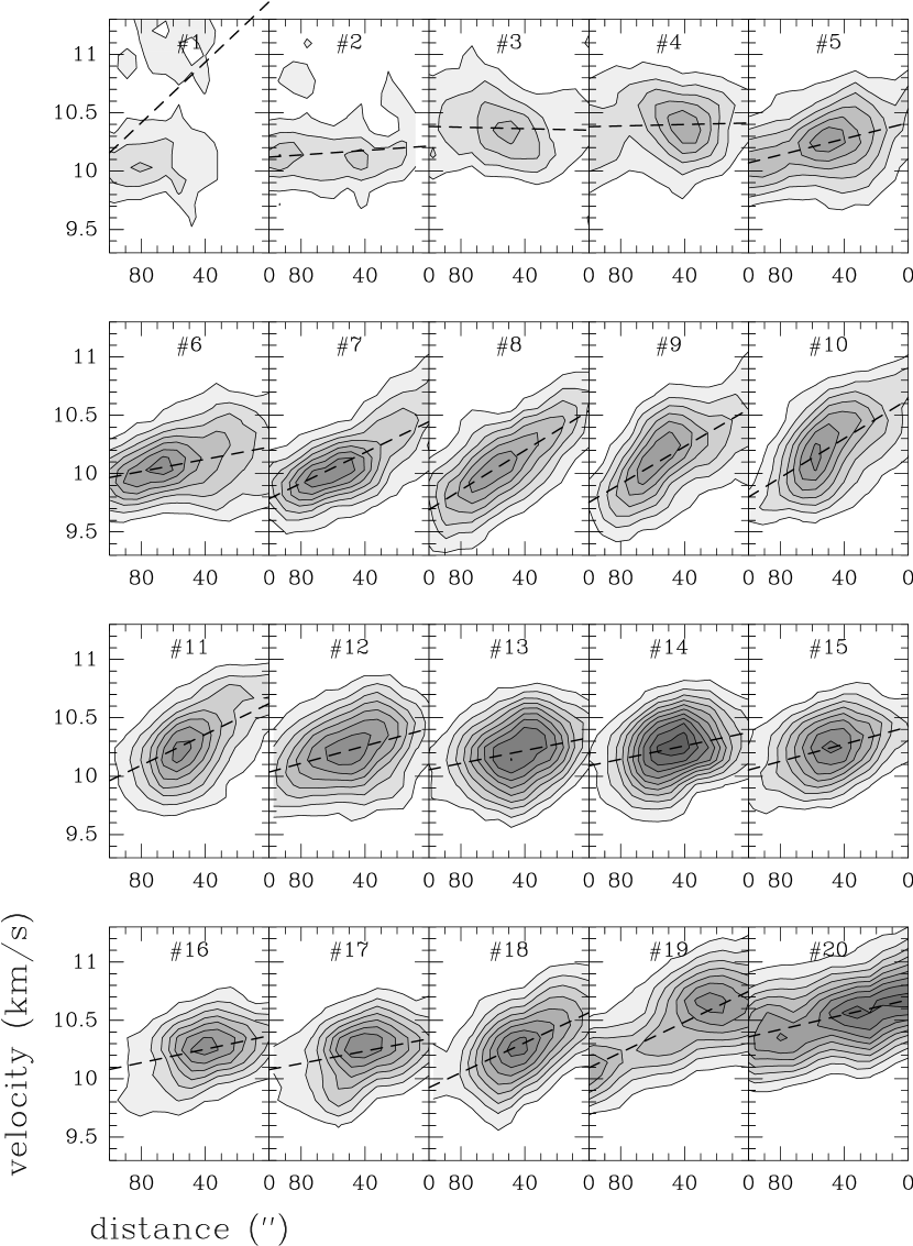
Figure 8: Transverse ${\rm C^{18}O}$$(2-1)$ position-velocity cuts performed across the neck, corresponding to the black thin lines of Fig. 5. The cuts are separated by 22^′′. The x-axis offsets increase northwise, so that the velocity decreases from South to North. Dashed lines indicate the results of the bi-dimensional fits to the $l-v$ diagram (see text for details), showing how the radial velocity gradient evolves as one moves from East to West (cf Fig. 9). Contours start at 3$\sigma$ (0.6 K), in steps of 3$\sigma$.

It is also interesting to compare the ratio of the gravitational to centrifugal forces in various areas of the Horsehead. This ratio is given by $\zeta=\pi G\langle\rho\rangle/\omega^{2}$ (with $\langle\rho\rangle$ the mean mass density and $\omega$ the angular velocity), translating into $\zeta\approx 10$ in the outer neck, while $\zeta\approx 1$ near Peak2. This means that gravity is able to ensure the confinement in the outer neck, while it is only marginally sufficient near Peak2.

5 Discussion

5.1 Formation and evolution of the Horsehead nebula

In the scenario proposed by Reipurth & Bouchet (1984), the Horsehead is assimilated to an early Bok globule emerging from its parental cloud via the eroding incident radiation field emitted by $\sigma$Ori. These authors also propose that the jaw cavity was the result of a collimated outflow, but this seems now highly unlikely (e.g.  Warren-Smith et al., 1985). Based on their CO$(1-0)$ data, PRB03 discuss the possible origin of this dark cloud, and conclude that both the work of instabilities and of the ionization front could be considered. They propose that the initial density enhancement in the parental cloud was asymmetric, at least at the western end of the neck, and that this material has been pushed out on either side of the neck, resulting in the mane and the jaw. They also deduce that the Horsehead’s neck is not axisymmetric but rather presents an oval cross-section. Their conclusions are, however, related to the general shape of the cloud, so they may have missed some of the details in the inner layers of the cloud due to the high opacity of their tracer. The data obtained in ${\rm C^{18}O}$ thus shed new light on the formation and evolution of the Horsehead.

Based on the velocity cuts described in the previous sections, the overall picture is that of an elongated structure (the neck) spinning around its own axis, and connected at its western end to a ridge (mane to nose) in rotation around this same axis. We found that this filament is roughly axisymmetric with a projected diameter $D\approx 0.15$ pc and a depth $L\approx 0.15-0.30$ pc. In the PRB03 scenario, all that is needed is some asymmetry at the front end of the neck, therefore it is not inconsistent with the present conclusion.

The reason the Horsehead followed such a peculiar route from L1630 might be linked to a pre-existing rotating velocity field in the region of the parental cloud that resisted the incident radiation field and gave birth to the protrusion, a possibility also mentioned by PRB03. As rotation proceeded, the centrifugal force has progressively detached the nose and the mane from the neck. This scenario requires initial density inhomogeneities within the pillar: the densest parts have formed the neck, mane, and nose, while the most tenuous ones remained as the jaw cavity and the optical hole. We note that this inhomogeneity is also required by the scenario reported by PRB03. This picture is moreover consistent with the gradient seen in the longitudinal $l-v$ cut shown in Fig. 6: the material extending from the nose down to the middle of the PDR (offsets 0 to 200^′′) is rotating, with the nose blue-shifted and part of the mane red-shifted. The southern end of the mane (offsets 200 to 300 ^′′ in Fig 6) is, however, braked back to the neck velocity. This suggests that part of the mane has remained attached to the pillar (their physical link is already obvious from various tracers, see Fig. 1), resulting in the material loop seen e.g. in the optical. As a consequence of this mechanism, the nose and the mane cannot lie in the plane of the sky as the neck presumably does. Rather, the nose would be in the foreground, while part of the mane would be in the background. The fact that the nose appears totally detached from the neck also indicates that the material void associated to the actual jaw was more pronounced than that in the optical hole. Obviously, the continued eroding work of $\sigma$Ori has proceeded during this process. It must thus have also contributed to the shaping of the structure we see in projection on the plane of the sky. This must be particularly true in the jaw and the optical hole, where the initial density contrast within the pristine pillar may thus have been enhanced.

In complement to this effect, the nose may also be pushed towards us by the rocket effect resulting from eventual background ionization. However, the amplitude of this effect must be negligible with respect to the prevailing velocity field since part of the mane remains red-shifted. Moreover, the rocket effect would also affect the neck which is seen to be rotating. We therefore discard the possibility of a non-negligible background ionization flux.

5.2 Rotation vs shear

We discuss here the question whether the velocity gradient revealed in the neck could be the signature of a velocity shear in a direction perpendicular to both the neck and the line of sight, rather than a rotation of the filamentary neck. We see at least three arguments favouring the rotation interpretation.

First of all, we have proposed in the previous section that both the (likely combined) effect of an abrasive ionizing front and that of a pre-existing velocity field may have contributed to the peculiar shaping of the Horsehead nebula. It is very unlikely that the ionization front arising from $\sigma$Ori could have generated a shear perpendicular to the line-of-sight, so that a velocity shear present in the neck should have its origin in the parental cloud. A careful look at the position-velocity cuts of Kramer et al. (1996) in ${\rm{}^{13}CO}$$(2-1)$ show no velocity gradient in the vicinity of the Horsehead nebula (Right Ascension offsets between -4 and -12 arcmin). There would thus be no shear in the parental cloud, and these would likely discard its existence in the neck.

A second argument consists in considering the morphological consequence of such a shear. Indeed, after some time, a shear in the neck would result in a filament far from being cylindrical, which is in disagreement with the result inferred from the column density calculation. The timescale for this motion can be roughly estimated from that of momentum transfer between the ionized and the condensed and cold gas. Assuming an average collisional cross-section for H–H⁺ encounters, $\langle u\sigma\rangle=2.2\times 10^{-9}{\rm cm^{-3}}\,$s (Spitzer, 1978), and adopting a mean density of proton $n_{f}$ as found in the Horsehead, one yields $\Delta t\approx 2/(n_{f}\langle u\sigma\rangle)\approx{\rm 10^{6}}$s, which even if underestimated by orders of magnitude, would be short enough by far to have disrupted the cylinder shape one still sees today.

Finally, if despite the arguments given above, shear would still play a role in the dynamic at work in the neck, and the torque it would exert on the mane and nose would in any case result in rotation in the filament.

Figure 9: Evolution of the transverse velocity gradient with the distance along the neck. The gradients and associated error bars were computed following the method described in Sect. 4.2. The dashed line shows the constant gradient of +1.5 ${\rm km\,s^{-1}\,pc^{-1}}$, indicating the area suggestive of rigid body rotation. Also shown are the peaks discussed in this paper. Some cut numbers are recalled for the purpose of comparison.

5.3 Dense core formation in the Horsehead

Dense cores are routinely observed in filaments; however, what triggers their formation is still an open issue. Fragmentation of gaseous cylinders resulting from periodic instabilities is often invoked, but their nature is uncertain, be they gravitationally or magnetically dominated, or even a combination of both. Determining the balance between these two forces appears to be a critical issue.

We have shown that the Horsehead neck is a filament harboring (at least) four density peaks (as evidenced by both 1.2mm and ${\rm C^{18}O}$ maps). The longitudinal cuts in the neck (Fig. 7) show that the longitudinal velocity is not uniform but instead varies periodically in the inner neck (period $\approx 0.3$ pc), around $V=10.2$ ${\rm km\,s^{-1}}$ close to the systemic velocity. This indicates that the filament is not located strictly in the plane of the sky. This oscillation could be explained considering matter that flows along a filament regularly bent with respect to the plane of the sky. Moreover, it is worth mentioning the presence of line wings around Peak3 (see offsets (200^′′,80^′′) in Fig. 4). However, the spatial resolution of our data is not sufficient to conclude a scenario such as outflow or inflow.

The radial cuts shown in Fig. 8 indicate that the phenomena at work are more complex: the longitudinal gradients are combined to rotation. This rotation is mainly that of a rigid body, although the angular velocity experiences a sharp increase from 1.5 to 4 ${\rm km\,s^{-1}\,pc^{-1}}$ (Fig. 8 and Fig. 9). Interestingly, the longitudinal gradient appears to change signs at the positions of Peak3 and 4 (Fig. 7), positions that also appear to play a particular role in the picture of radial gradients (Fig. 9). It suggests a dynamical link between the formation of the condensations observed in the neck and the material flow revealed by the complex velocity structure of the filament. Finally, we note that another likely effect of the combination of both longitudinal and radial motions is the morphology change observed between, e.g., cuts #8 and #14 (Fig. 8): cut #14 is much more rounded than the straight contours of cut #8. At this stage it becomes difficult to derive an accurate picture accounting for the combination of all these phenomena. We believe that detailed interpretation of all these signatures requires dedicated numerical modelling.

We can, however, already infer preliminary constraints about some of the principal ingredients of this modelling, namely gravity and magnetic field. In cylindrical geometry, the virial mass per unit length may be written (e.g. Fiege & Pudritz, 2000):

$$m_{\rm vir}=\frac{2\langle\sigma^{2}\rangle}{G}.$$ (1)

Assuming $\langle\sigma^{2}\rangle\approx\sigma_{v}^{2}$, this gives

$$m_{\rm vir}=4.6\left(\frac{\sigma_{v}}{0.1\,{\rm km\,s^{-1}}}\right)^{2}\,\,\rm M_{\odot}/pc.$$ (2)

For the velocity dispersion, we apply the Fuller & Myers (1992) formula:

$$\sigma_{v}^{2}=\sigma_{v,\rm obs}^{2}+k_{B}T_{{\rm kin}}\left(\frac{1}{\tilde{m}}-\frac{1}{m_{\rm obs}}\right)$$ (3)

where ${\tilde{m}}$ is the mean mass of molecular gas, taken here equal to 2.33; $m_{\rm obs}$ is the mass of the molecular tracer namely ${\rm C^{18}O}$; and $T_{{\rm kin}}$ the kinetic temperature. We adopt $T_{{\rm kin}}$ = 20K and $\sigma_{v,\rm obs}=0.66/2.35$ ${\rm km\,s^{-1}}$, resulting in a virial mass $m_{\rm vir}\approx 65\rm M_{\odot}/$pc. On the other hand, the mass per unit length we can deduce from the density and size (see Sect. 3.2) is

$$m=18\,\,\left(\frac{n_{{\rm H}}}{{\rm 10^{4}}\,{\rm cm^{-3}}}\right)\left(\frac{R}{0.1\,pc}\right)\,\,\rm M_{\odot}/pc.$$ (4)

Taking $n_{{\rm{\rm H_{2}}}}$ = 5$\times 10^{3}$ ${\rm cm^{-3}}$ and $R\approx 0.2$ pc results in mass per unit length $m\approx$ 20 $\rm M_{\odot}$/pc. The filament is not self-gravitating, since $m/m_{\rm vir}\approx 0.3$. This value falls in the range of ratio presented by Fiege & Pudritz (2000). This again raises the question of the confinement of the filament. However, the ratio is not that small, and the gravity is expected to play a role in the dynamics of the filament.

To our knowledge, no estimation of the magnetic field strength is available for the Horsehead. Polarized absorbed starlight is reported in Warren-Smith et al. (1985), completed by the large-scale dataset of Zaritsky et al. (1987). In the Horsehead, the polarization is probably due only to alignment of absorbing dust grains. The transmitted light is therefore aligned with the magnetic fields projected on the plane of the sky. Obviously, this technique does not allow detection of any polarization in the densest parts of the Horsehead. The overall picture is that of a $\@vec{B}$-field oriented nearly North-South i.e. perpendicular to the filament. Moreover, it coincides with the large-scale field. In the nose area, however, the polarization vectors appear perpendicular to the structure with an angle $\approx 45^{\circ}$ with respect to the large-scale field. The nose may thus have bent the field lines in its centrifugal motion. In the filament, though, we cannot yet distinguish between a toroidal component threading the neck and pure transverse magnetic field across the neck itself. It is worth noting that the same is observed in some dark clouds in the Taurus and in Ophiuchus: the magnetic fields orientation at the scale of the dark clouds fits into smooth, larger-scale fields. In the Taurus, the magnetic fields appear perpendicular to the cloud’s long axis, while in Ophiuchus it would be parallel (Heiles et al., 1992).

We therefore think that both gravity and magnetic fields are expected to play a role in the confinement and dense core formation in the Horsehead nebula.

6 Conclusions

We have studied the morphology and velocity structure of the Horsehead nebula using new observations at high frequency and spatial resolution in the $(2-1)$ transition of ${\rm C^{18}O}$. Our conclusions can be summarized as follows:

1. the emission of the likely optically thin tracer reveals a filamentary morphology similar to the one seen in dust millimetre continuum emission and visual extinction. The cloud appears as a curved ridge (the PDR) connected to L1630 by a thin (0.15 pc diameter) pillar hosting several condensations. One of them (Peak2) also appears in absorption in the mid-IR emission at 7 $\mu$m.

2. we note that our thin ${\rm C^{18}O}$$(2-1)$ map is much less clumpy than the possibly thick ${\rm{}^{12}CO}$$(1-0)$ from PRB03, a phenomenon that could be due to either excitation or photodissociation selective effects or the combination of both.

3. these cores are density peaks ($n_{\rm H_{2}}$ in the range $2-4\times 10^{4}$ ${\rm cm^{-3}}$) embedded in a medium that is more diffuse by a factor of 2-3 on average. Kinetic temperatures in these cores are found in the range 20-30 K, although the brightest of them (Peak2) shows hints of ${\rm C^{18}O}$ depletion onto grains, pointing towards a somewhat colder environment.

4. the overall shape of the filament is found to be fairly cylindrical with a diameter of about 0.15–0.30 pc. The total mass of the ${\rm C^{18}O}$ gas probed here is 20 $\rm M_{\odot}$, of which the largest fraction was found to be in the gaseous phase.

5. the centroid velocity map suggests that the gas in the Horsehead is wrapped around an axis coincident with the pillar. The cloud also presents various velocity gradients along the filaments described above. While the western ridge presents two strong north-south gradients inverting sign at the rise of the mane, the east-west pillar exhibits a more complex shape where gradient oscillations occur on a regular basis and seem bracketed by the location of the embedded condensations.

6. tranverse gradients are prominent almost everywhere across the pillar, but some of them depart from linear shape and might indicate differential rotation. The amplitude of the gradient is on average constant (1.5 ${\rm km\,s^{-1}\,pc^{-1}}$, corresponding to a rotation period of 4 Myrs, comparable to the 5 Myrs lifetime estimated by PRB03) at either end of the neck, but a sharp increase to 4 ${\rm km\,s^{-1}\,pc^{-1}}$ is observed between two of the embedded peaks. Reasons for this peculiar behaviour are still unclear.

7. this complex dynamic picture raises the question of whether the origin of this protrusion could be linked to a pre-existent velocity field that progressively separated the mane and nose from the neck via centrifugal effects. The presence of several condensations unveiled inside the filament also supports the idea that dense cores are forming in the neck, and their characteristics share several similarities with modelling works on that topic. Their origin is very likely due to the combination of longitudinal (infall) and radial motions, but the actual phenomena at work may even be more complex, as the magnetic field is expected to also play a role in this process. Moreover, the origin of the initial velocity field invoked in this work remained unknown.

Firmer conclusions on the formation scenario of such a protrusion should, however, await comparison with numerical models, and the relatively simple geometry of the Horsehead neck should be a particularly appealing application.