Cosmological constraints from galaxy clustering

1 Abstract

In this manuscript I review the mathematics and physics that underpins recent work using the clustering of galaxies to derive cosmological model constraints. I start by describing the basic concepts, and gradually move on to some of the complexities involved in analysing galaxy redshift surveys, focusing on the 2dF Galaxy Redshift Survey (2dFGRS) and the Sloan Digital Sky survey (SDSS). Difficulties within such an analysis, particularly dealing with redshift space distortions and galaxy bias are highlighted. I then describe current observations of the CMB fluctuation power spectrum, and consider the importance of measurements of the clustering of galaxies in light of recent experiments. Finally, I provide an example joint analysis of the latest CMB and large-scale structure data, leading to a set of parameter constraints.

2 introduction

The basic techniques required to analyse galaxy clustering were introduced in the 70s peebles73 , and have been subsequently refined to match data sets of increasing quality and size. In this manuscript I have tried to summarise the current state of this field. Obviously, such an attempt can never be complete or unique in every detail, although it is still worthwhile as it is always useful to have more than one source of information. An excellent alternative viewpoint was recently provided by Hamilton hamilton1 ; hamilton2 , which covers some of the same material, and provides a more detailed review of some of the statistical methods that are used. Additionally it is worth directing the interested reader to a number of good text books that cover this topic coles_lucchin ; dodelson ; liddle_lyth ; book_of_john . In addition to a description of the basic mathematics and physics behind a clustering analysis I have attempted to provide a discussion of some of the fundamental and practical difficulties involved. The cosmological goal of such an analysis is consider in the final part of this manuscript, where the combination of cosmological constraints from galaxy clustering and the CMB is discussed, and an example multi-parameter fit to recent data is considered.

3 Basics

Our first step is to define the dimensionless overdensity

$$\delta({\bf x})=\frac{\rho({\bf x})-\bar{\rho}}{\bar{\rho}},$$ (1)

where $\bar{\rho}$ is the expected mean density, which is independent of position because of statistical homogeneity.

The autocorrelation function of the overdensity field (usually just referred to as the correlation function) is defined as

$$\xi(\mathbf{x_{1}},\mathbf{x_{2}})\equiv\left\langle\delta(\mathbf{x_{1}})\delta(\mathbf{x_{2}})\right\rangle.$$ (2)

From statistical homogeneity and isotropy, we have that

$$\xi(\mathbf{x_{1}},\mathbf{x_{2}}) = \xi(\mathbf{x_{1}}-\mathbf{x_{2}}),$$ (3)

$$= \xi(|\mathbf{x_{1}}-\mathbf{x_{2}}|).$$ (4)

To help to understand the correlation function, suppose that we have two small regions $\delta V_{1}$ and $\delta V_{2}$ separated by a distance $r$. Then the expected number of pairs of galaxies with one galaxy in $\delta V_{1}$ and the other in $\delta V_{2}$ is given by

$$\left\langle n_{\rm pair}\right\rangle=\bar{n}^{2}\left[1+\xi(r)\right]\delta V_{1}\delta V_{2},$$ (5)

where $\bar{n}$ is the mean number of galaxies per unit volume. We see that $\xi(r)$ measures the excess clustering of galaxies at a separation $r$. If $\xi(r)=0$, the galaxies are unclustered (randomly distributed) on this scale – the number of pairs is just the expected number of galaxies in $\delta V_{1}$ times the expected number in $\delta V_{2}$. $\xi(r)>0$ corresponds to strong clustering, and $\xi(r)<0$ to anti-clustering. Estimation of $\xi(r)$ from a sample of galaxies will be discussed in Section 6.1.

It is often convenient to consider perturbations in Fourier space. In cosmology the following Fourier transform convention is most commonly used

$$\delta({\bf k}) \equiv \int\delta({\bf r})e^{i{\bf k.r}}d^{3}r$$ (6)

$$\delta({\bf r}) = \int\delta({\bf k})e^{-i{\bf k.r}}\frac{d^{3}k}{(2\pi)^{3}}.$$ (7)

The power spectrum is defined as

$$P({\bf k_{1}},{\bf k_{2}})=\frac{1}{(2\pi)^{3}}\left\langle\delta({\bf k_{1}})\delta({\bf k_{2}})\right\rangle.$$ (8)

Statistical homogeneity and isotropy gives that

$$P({\bf k_{1}},{\bf k_{2}})=\delta_{D}({\bf k_{1}}-{\bf k_{2}})P(k_{1}),$$ (9)

where $\delta_{D}$ is the Dirac delta function. The power spectrum is sometimes presented in dimensionless form

$$\Delta^{2}(k)=\frac{k^{3}}{2\pi^{2}}P(k).$$ (10)

The correlation function and power spectrum form a Fourier pair

$$P(k) \equiv \int\xi(r)e^{i{\bf k.r}}d^{3}r$$ (11)

$$\xi(r) = \int P(k)e^{-i{\bf k.r}}\frac{d^{3}k}{(2\pi)^{3}},$$ (12)

so they provide the same information. The choice of which to use is therefore somewhat arbitrary (see hamilton1 for a further discussion of this).

The extension of the 2-pt statistics, the power spectrum and the correlation function, to higher orders is straightforward with Eq. 5 becoming

$$\left\langle n_{\rm tuple}\right\rangle=\bar{n}^{n}\left[1+\xi^{(n)}\right]\delta V_{1}\cdot\cdot\cdot\delta V_{n}.$$ (13)

However, the central limit theorem implies that a density distribution is asymptotically Gaussian in the limit where the density results from the average of many independent processes. The overdensity field has zero mean by definition, so is completely characterised by either the correlation function or the power spectrum. Consequently, in this regime, measuring either the correlation function or the power spectrum provides a statistically complete description of the field.

4 matter perturbations

Figure 1: Plots showing the linear power spectrum (solid lines) for a variety of different cosmological parameters. Only the shapes of the power spectra are compared, and the amplitudes are matched to the same large scale value. Our base model has $\Omega_{M}h=0.2$, $n_{s}=1$, $\Omega_{b}/\Omega_{M}=0$ and $\Omega_{\nu}/\Omega_{M}=0$. Deviations from this base model are given in each panel. As can be seen many of the shape distortions from changing different parameters are similar, which can cause degeneracies between these parameters when fitting models to observations.

There are three physical stages in the creation and evolution of perturbations in the matter distribution. First, primordial perturbation are produced in an inflationary epoch. Second, the different forms of matter within the Universe affect these primordial perturbations. Third, gravitational collapse leads to the growth of these fluctuations. In this section we will discuss the form of the perturbations on scales where gravitational collapse can be described by a linear change in the overdensity. The gravitational collapse of perturbations will be considered in Section 5.

4.1 why are there matter perturbations?

A period of “faster than light” expansion in the very early Universe solves a number of problems with standard cosmology. In particular, it allows distant regions that appear causally disconnected to have been connected in the past and therefore explains the flatness of the CMB. Additionally it drives the energy density of the Universe close to the critical value and, most importantly for our discussion of perturbations, it provides a mechanism for producing seed perturbations as quantum fluctuations in the matter density are increased to significant levels. For a detailed examination of the creation of fluctuations see liddle93 . For now, we will just comment that the most basic inflationary models give a spectrum of fluctuations $P(k)\propto k^{n}$ with $n\sim 1$.

4.2 the effect of dark matter

The growth of dark matter fluctuations is intimately linked to the Jeans scale. Perturbations smaller than the Jeans scale do not collapse due to pressure support – for collision-less dark matter this is support from internal random velocities. Perturbations larger than the Jeans scale grow through gravity at the same rate, independent of scale. In a Universe with just dark matter and radiation, the Jeans scale grows to the size of the horizon at matter-radiation equality, and then reduces to zero when the matter dominates. We therefore see that the horizon scale at matter-radiation equality will be imprinted in the distribution of fluctuations – this scale marks a turn-over in the growth rate of fluctuations. What this means in practice is that there is a cut-off in the power spectrum on small scales, dependent on $\Omega_{M}h$, with a stronger cut-off predicted for lower $\Omega_{M}h$ values. This is demonstrated in Fig. 1.

4.3 the effect of baryons

At early epochs baryons are coupled to the photons and, if we consider a single fluctuation, a spherical shell of gas and photons is driven away from the perturbation by a sound wave. When the photons and gas decouple, a spherical shell of baryons is left around a central concentration of dark matter. As the perturbation evolves through gravity, the density profiles of the baryons and dark matter grow together, and the perturbation is left with a small increase in density at a location corresponding to the sound horizon at the end of the Compton drag epoch bashinsky1 ; bashinsky2 . This real-space “shell” is equivalent to oscillations in the power spectrum. In addition to these acoustic oscillations, fluctuations smaller than the Jeans scale, which tracks the sound horizon until decoupling, do not grow, while large fluctuations are unaffected and continue to grow. The presence of baryons therefore also leads to a reduction in the amplitude of small scale fluctuations. For more information and fitting formulae for the different processes a good starting point is eh98 .

4.4 the effect of neutrinos

The same principal of gravitational collapse versus pressure support can be applied in the case of massive neutrinos. Initially the neutrinos are relativistic and their Jeans scale grows with the horizon. As their temperature decreases their momenta drop, they become non-relativistic, and the Jeans scale decreases – they can subsequently fall into perturbations. Massive neutrinos are interesting because even at low redshifts the Jeans scale is cosmologically relevant. Consequently the linear power spectrum (the fluctuation distribution excluding the non-linear collapse of perturbations) is not frozen shortly after matter-radiation equality. Instead its form is still changing at low redshifts. Additionally, the growth rate depends on the scale - it is suppressed until neutrinos collapse into perturbations, simply because the perturbations have lower amplitude. The effect of neutrino mass on the present day linear power spectrum is shown in Fig. 1. Note that in this plot the relative amplitudes of the power spectra have been removed - it is just the shape that is compared. The amplitude would also depend on the combined neutrino mass.

5 the evolution of perturbations

Having discussed the form of the linear perturbations, we will now consider how perturbations evolve through gravity in the matter and dark energy dominated regimes. To do this, we will use the spherical top-hat collapse model, where we compare a sphere of background material with radius $a$, with one of radius $a_{p}$ which contains the same mass, but has a homogeneous change in overdensity. The ease with which the behaviour can be modeled follows from Birkhoff’s theorem, which states that a spherically symmetric gravitational field in empty space is static and is always described by the Schwarzchild metric birkhoff23 . This gives that the behaviour of the homogeneous sphere of uniform density and the background can be modeled using the same equations. For simplicity we initially only consider the sphere of background material.

The sphere of background material behaves according to the standard Friedmann and cosmology equations

$$E^{2}(a)=\frac{1}{a^{2}}\left(\frac{da}{dH_{0}t}\right)^{2}=\Omega_{M}a^{-3}+\Omega_{K}a^{-2}+\Omega_{X}a^{f(a)},$$ (14)

$$\frac{1}{a}\frac{d^{2}a}{dt^{2}}=-\frac{H_{0}^{2}}{2}\left[\Omega_{M}a^{-3}+[1+3w(a)]\Omega_{X}a^{f(a)}\right].$$ (15)

These equations have been written in a form allowing for a general time-dependent equation of state for the dark energy $p=w(a)\rho$. Conservation of energy for the dark energy component provides the form of $f(a)$

$$f(a)=\frac{-3}{\ln a}\int_{0}^{\ln a}\left[1+w(a^{\prime})\right]d\ln a^{\prime}.$$ (16)

The dark matter and dark energy densities evolve according to

$$\Omega_{M}(a)=\frac{\Omega_{M}a^{-3}}{E^{2}(a)},\,\,\,\Omega_{X}(a)=\frac{\Omega_{X}a^{f(a)}}{E^{2}(a)}.$$ (17)

Tracks showing the evolution of $\Omega_{M}(a)$ and $\Omega_{X}(a)$ are presented in Fig. 2 for $h=0.7$ and constant dark energy equation of state $w=-1$.

Figure 2: Plot showing the evolution of the matter and vacuum energy densities for a selection of cosmologies (grey lines) with constant dark energy equation of state parameter $w=-1$. The critical models that border the different types of evolution are shown by the black lines. The dotted line highlights $\Omega_{X}=0$.

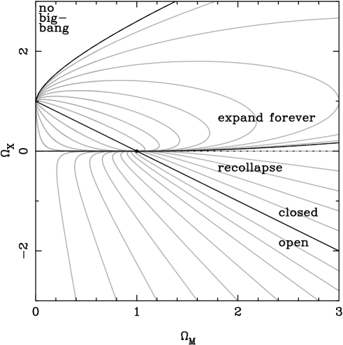
Of particular interest are solutions which predict recollapse, but that have $\Omega_{X}>0$. Provided that $\Omega_{M}>>\Omega_{X}$, the perturbation will collapse before the dark energy dominates. For a cosmology with $\Omega_{M}\sim 0.3$ and $\Omega_{X}\sim 0.7$, these solutions correspond to overdense spheres that will collapse and form structure.

For the perturbation, the cosmology equation can be written

$$\frac{1}{a_{p}}\frac{d^{2}a_{p}}{dt^{2}}=-\frac{H_{0}^{2}}{2}\left[\Omega_{M}a_{p}^{-3}+[1+3w(a)]\Omega_{X}a^{f(a)}\right],$$ (18)

where it is worth noting that the dark energy component is dependent on $a$ rather than $a_{p}$. This does not matter for $\Lambda$-cosmologies as $f(a)=0$, and the $a$ dependence in this term is removed. For other dark energy models, this dependence follows if the dark energy does not cluster on the scales of interest. For such cosmological models, we cannot write down a Friedmann equation for the perturbation because energy is not conserved wang98 . We also have to be more careful using virialisation arguments to analyse the behaviour of perturbations percival05 .

To first order, the overdensity of the perturbation $\delta=a^{3}/a_{p}^{3}-1$ evolves according to

$$\frac{d^{2}\delta}{d(H_{0}t)^{2}}+\frac{2}{a}\frac{da}{d(H_{0}t)}\frac{d\delta}{d(H_{0}t)}-\frac{3}{2}\Omega_{M}a^{-3}\delta=0,$$ (19)

which is known as the linear growth equation.

Figure 3: Plot showing the evolution of the scale factor of perturbations with different initial overdensities. A standard cosmology with $\Omega_{M}=0.3$, $\Omega_{X}=0.7$, $h=0.7$, $w=-1$ is assumed. The dashed lines show the linear extrapolation of the perturbation scales for the two least overdense perturbations.

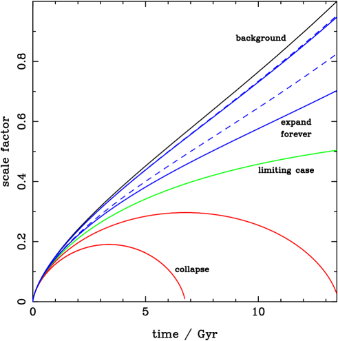
The evolution of the scale factor of the perturbations is given by the solid lines in Fig. 3, compared with the background evolution for a cosmology with $\Omega_{M}=0.3$, $\Omega_{X}=0.7$, $h=0.6$, $w=-1$. These data were calculated by numerically solving Eq. 18. For comparison, the dashed lines were calculated by extrapolating the initial perturbation scales using the linear growth factor, calculated from Eq. 19. Dashed lines are only plotted for the two least overdense perturbations. In comparison, the most overdense perturbations are predicted to collapse to singularities. However, in practice inhomogeneities, and the non-circular shape of actual perturbations will mean that the object virialises with finite extent.

The evolution of perturbations has a profound affect on the present day power spectrum of the matter fluctuations on small scales. On the largest scales, the overdensities are small and linear theory (Eq. 19) holds. This increases the amplitude of the fluctuations, but does not change the shape of the power spectrum, as the perturbation all grow at the same rate (except if neutrinos are cosmologically relevant – see Section 4.4). However, on the smallest scales, overdensities are large and collapse to virialised structures (e.g. cluster of galaxies). The effect on the power spectrum is most easily quantified using numerical simulations, and power spectra calculated from fitting formulae derived from such simulations smith03 are plotted in Fig. 4.

Figure 4: Plots comparing non-linear (solid lines) and linear power spectra (dotted lines) at a series of redshifts from $z=0$ to $z=5$. In the left panel the raw dimensionless power spectra are plotted while in the right panel the ratio between non-linear and linear predictions is shown. As can be seen, on large scales linear growth simply increases the amplitude of the power spectrum, while on small scales we also see an increase in power as structures collapse at low redshifts. There is also a slight decrease in power on intermediate scales – it is this power that is transferred to small scales. Non-linear power spectra were calculated from the fitting formulae of smith03 with $\Omega_{M}=0.3$, $h=0.7$, $n_{s}=1$, and $\Omega_{b}/\Omega_{m}=0.15$.

6 galaxy survey analysis

6.1 estimating the correlation function

First suppose that we have a single population of objects forming a Poisson sampling of the field that we wish to constrain. This is too simple an assumption for the analysis of modern galaxy redshift surveys, but it will form a starting point for the development of the analysis tools required.

First we define the (unweighted) galaxy density field

$$n_{g}({\bf r})\equiv\sum_{i}\delta_{D}({\bf r}-{\bf r_{i}}).$$ (20)

The definition of the correlation function then gives

$$\left\langle n_{g}({\bf r})n_{g}({\bf r^{\prime}})\right\rangle=\bar{n}({\bf r})\bar{n}({\bf r^{\prime}})[1+\xi({\bf r}-{\bf r^{\prime}})]+\bar{n}({\bf r})\delta_{D}({\bf r}-{\bf r^{\prime}}).$$ (21)

The final term in this equation relates to the shot noise, and only occurs for zero separation so can be easily dealt with.

In order to estimate the correlation function, we can consider a series of bins in galaxy separation and make use of Eq. 21. Suppose that we have created a (much larger) random distribution of points that form a Poisson sampling of the volume occupied by the galaxies, then

$$1+\xi=\frac{\left\langle DD\right\rangle}{\left\langle RR\right\rangle}(1+\xi_{\Omega}),$$ (22)

where $DD$ is the number of galaxy-galaxy pairs within our bin in galaxy separation divided by the maximum possible number of galaxy-galaxy pairs (ie. for $n$ galaxies the maximum number of distinct pairs is $n(n-1)/2$). Similarly $RR$ is the normalised number of random-random pairs, and we can also define $DR$ as the normalised number of galaxy-random pairs.

If the true mean density of galaxies $\bar{n}({\bf r})$ is estimated from the sample itself (as is almost always the case), we must include a factor $(1+\xi_{\Omega})$ that corrects for the systematic offset induced. $\xi_{\Omega}$ is the mean of the two-point correlation function over the sampling geometry landy93 . Given only a single clustered sample it is obviously difficult to determine $\xi_{\Omega}$, and the integral constraint (as it is known) remains a serious drawback to the determination of the correlation function from small samples of galaxies.

Because the galaxy and random catalogues are uncorrelated, $\left\langle DR\right\rangle=\left\langle RR\right\rangle$, and we can consider a number of alternatives to Eq. 22. In particular

$$1+\xi=\left(1+\frac{\left\langle(D-R)^{2}\right\rangle}{\left\langle RR\right\rangle}\right)(1+\xi_{\Omega}),$$ (23)

has been shown to have good statistical properties landy93 .

6.2 estimating the power spectrum

In this section we consider estimating the power spectrum by simply taking a Fourier transform of the overdensity field baumgart91 ; FKP ; PVP . As for our estimation of the correlation function, suppose that we have quantified the volume occupied by the galaxies by creating a large random catalogue matching the spatial distribution of the galaxies, but with no clustering (containing $\alpha$ times as many objects). The (unnormalised) overdensity field is

$$F({\bf r})=n_{g}({\bf r})-n_{r}({\bf r})/\alpha,$$ (24)

where $n_{g}$ is given by Eq. 20, and $n_{r}$ is similarly defined for the random catalogue.

Taking the Fourier transform of this field, and calculating the power gives

$$\left\langle|F({\bf k})|^{2}\right\rangle=\int\frac{d^{3}k^{\prime}}{(2\pi)^{3}}[P({\bf k^{\prime}})-P(0)\delta_{D}({\bf k})]|G({\bf k}-{\bf k^{\prime}})|^{2}+(1+\frac{1}{\alpha})\int d^{3}r\bar{n}({\bf r}),$$ (25)

where $G({\bf k})$ if the Fourier transform of the window function, defined by

$$G({\bf k})\equiv\int\bar{n}({\bf r})e^{i{\bf k.r}}d^{3}r,$$ (26)

and the final term in Eq. 25 gives the shot noise. In contrast to the correlation function, there is a shot noise contribution at every scale. The integral constraint has reduced to subtracting a single Dirac delta function from the centre of the unconvolved power - as before this allows for the fact that we do not know the mean density of galaxies.

6.3 complications

There are two complications which constitute the main hindrance to using clustering in galaxy surveys to constrain cosmology. They are redshift space distortions – systematic deviations in measured redshift in addition to the Hubble flow, and galaxy bias – the fact that galaxies do not form a Poisson sampling of the underlying matter distribution. Denoting the measurement of a quantity in redshift space (galaxy distances calculated from redshifts) by a superscript ^s and in real space (true galaxy distances) by ^r, we can write the measured power spectrum $P_{\rm gal}^{s}$ as

$${P_{\rm gal}^{s}\over P_{\rm mass}}={P_{\rm gal}^{s}\over P_{\rm gal}^{r}}\times{P_{\rm gal}^{r}\over P_{\rm mass}}.$$ (27)

The first of these terms corresponds to redshift space distortions, while the second corresponds to galaxy bias.

redshift space distortions

There are two key mechanisms that systematically distort galaxy redshifts from their Hubble flow values. First, structures are continually growing through gravity, and galaxies fall into larger structures. The infall velocity adds to the redshift, making the distance estimates using the Hubble flow wrong. This means that clusters of galaxies appear thinner along the line-of-sight, causing an increase in the measured power. In the distant observer approximation, the apparent amplitude of the linear density disturbance can be readily calculated kaiser87 , leading to a change in the power corresponding to

$$P_{\rm gal}^{s}=P_{\rm gal}^{r}(1+\beta\mu^{2})^{2},$$ (28)

where $\beta=\Omega_{M}^{0.6}/b$, $b$ is an assumed linear bias for the galaxies, and $\mu$ is the cosine between the velocity vector and the line-of-sight. In the small angle approximation, we average over a uniform distribution for $\mu$ giving

$$P_{\rm gal}^{s}=P_{\rm gal}^{r}\left[1+\frac{2}{3}\beta+\frac{1}{5}\beta^{2}\right].$$ (29)

For large redshift surveys of the nearby Universe, the small angle approximation breaks down, although a linear result can be obtained using a spherical expansion of the survey (see Section 6.5).

When objects collapse and virialise they attain a distribution with some velocity dispersion. These random velocities smear out the collapsed object along the line of sight in redshift space, leading to the existence of linear structures pointing towards the observer. These structures, known as “fingers-of-god” can be corrected by matching with a group catalogue and applying a correction to the galaxy field before analysis tegmark04 . Alternatively, if the pairwise distribution of velocity differences is approximated by an exponential distribution, then

$$P_{\rm gal}^{s}=P_{\rm gal}^{r}(1+k^{2}\mu^{2}\sigma_{p}^{2}/2)^{-1},$$ (30)

where $\sigma_{p}\sim 400\,{\rm km\,s^{-1}}$ is the pairwise velocity dispersion hawkins03 .

galaxy bias

By the simple phrase “galaxy bias” astronomers quantify the “messy” astrophysics of galaxy formation. It is common to assume a local linear bias with $\delta_{\rm gal}=b\delta_{\rm mass}$, which leads to a simple relation between power spectra $P_{\rm gal}^{r}=b^{2}P_{\rm mass}$. If this bias is independent of the scale probed, then there is nothing to worry about – the galaxy and matter power spectra have the same shape. However, it is well known that galaxies of different types have different clustering strengths – two recent analyses are seaborne99 ; wild05 .

One simple way of understanding galaxy bias is to use the “halo model”, which has become popular over the last 5 years seljak00 ; peacock00 ; cooray02 . First, consider the distribution of the underlying matter – the power spectrum was shown in Fig. 4. There are two distinct regimes: on large scales, linear growth holds, while on small scales the dark matter has formed into halos: it has either undergone collapse and has virialised, or is on the way to virialisation. Galaxies pinpoint certain locations within the dark matter halos, according to an occupation distribution for each galaxy type. This forms a natural environment in which to model galaxy bias, with galaxies of different luminosities and types have different occupation distributions depending on the physics of their formation.

For 2-pt statistics, then there are two possibilities for pairs of galaxies. We could have chosen a pair where both galaxies lie in the same halo – this is most likely on small scales. Alternatively, the galaxies might be in different halos – this is most likely on large scales. On large scales, the halos themselves are biased compared with the matter and we can use the peak-background split model cole89 ; mo96 ; sheth99 to estimate the increase in clustering strength. This limiting large scale value offers a route to determine the masses of the virialised structures in which particular galaxies live.

Given a linear bias model for each type of galaxy in the sample to be analysed, it is possible to multiply the contribution of each galaxy to the estimate of the overdensity field by the inverse of an expected bias PVP . Provided the bias model is correct (and possibly altered for each scale observed), then this removes any systematic offset in the recovered power spectrum caused by galaxy bias. The problem is that we need to have an accurate model of the galaxy bias in order to remove it.

6.4 weights

The procedure described in Section 6.2 can be extended to include weights for each galaxy in order to optimise the analysis FKP . Under the assumptions that the wavelength of interest $2\pi/k$ is small compared with the survey scale (i.e. the window is negligible), and that the fluctuations are Gaussian, then the optimal weight applied to galaxy $i$ is

$$w_{i}=\frac{1}{1+\bar{n}({\bf r}_{i})\hat{P}(k)},$$ (31)

where $\bar{n}({\bf r}_{i})$ is the mean galaxy density at the location of galaxy $i$. At locations where the mean galaxy density is low, galaxies are weighted equally. Where the galaxy density is high, we weight by volume. It is worth noting that the optimal weights also depend on an estimate of the power spectrum to be measured, and therefore depend on the scale of interest. However, in practice this dependence is sufficiently weak that very little information is lost by assuming a constant $\hat{P}(k)$.

It is possible to include galaxy bias when determining weights and optimising the analysis in order to recover the most signal. Given a bias for each galaxy $b_{i}$ (which can be dependent on any galaxy properties and the scale of interest), then the optimal weighting is PVP .

$$w_{i}=\frac{b_{i}^{2}}{1+\sum_{j}\bar{n}({\bf r_{i}},b_{j})b_{j}^{2}\hat{P}(k)},$$ (32)

which up-weights the most biased galaxies that contain the strongest cosmological signal.

6.5 spherical bases

In Section 6.2 we described the most simple analysis method for a 3-dimensional galaxy survey – decomposing into a 3D Fourier basis. However, as we discussed in Section 6.3 redshift-space distortions complicate the situation, and cannot easily be dealt with using a Fourier basis. By decomposing into a basis that is separable in radial and angular directions, we can more easily correct such distortions. A pictorial comparison of the Fourier basis with a radial-angular separable basis is presented in Fig. 5.

Figure 5: Comparison of 3D Fourier basis split into 2D and 1D components (right) with basis of Spherical Harmonics (with $l=2$ and $m=0,1$ – top left) and Spherical Bessel functions (bottom left).

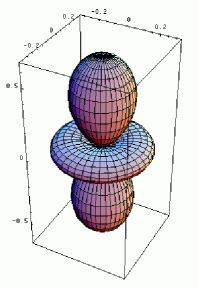
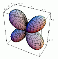
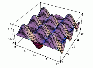
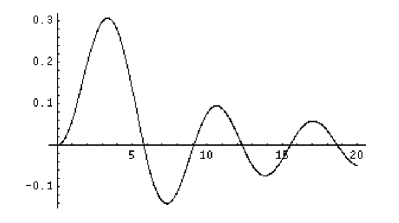
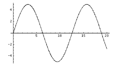
In this section we provide an overview of a formalism to do this based on work by heavens95 ; tadros99 ; percival04 . For alternative formalisms see fisher94 ; hamilton2 ; tegmark04 . In comparison with the Fourier decomposition (Eq. 6), we decompose into a 3D basis of Spherical Harmonics $Y_{lm}$ and spherical Bessel functions $j_{l}$

$$\delta(\mbox{\boldmath$x$})=\sqrt{\frac{2}{\pi}}\int^{\infty}_{0}\sum_{l,m}\delta_{lm}(k)j_{l}(kx)Y_{lm}(\theta,\phi)kdk.$$ (33)

Because of the choice of bases, the transformation $\delta_{lm}(k)\leftrightarrow k\delta(\mbox{\boldmath$k$})$ is unitary so we retain the benefit of working with the Fourier power spectrum

$$\left\langle\delta_{lm}(k)\delta_{l^{\prime}m^{\prime}}(k^{\prime})\right\rangle=P(k)\delta_{D}(k-k^{\prime})\delta_{D}(l-l^{\prime})\delta_{D}(m-m^{\prime}).$$ (34)

As in Section 6.2, we have simplified the analysis by not including any galaxy weights, although these can be introduced into the formalism. Additionally, it is easier to work with a fixed boundary condition - usually that fluctuations vanish at some large radius so that we are only concerned with radial modes that have

$$\left.\frac{d}{dx}j_{l}(kx)\right|_{x_{\rm max}}=0,$$ (35)

so that the decomposition becomes

$$\delta(\mbox{\boldmath$x$})=\sum_{l,m,n}c_{ln}\delta_{lmn}j_{l}(k_{ln}x)Y_{lm}(\theta,\phi),$$ (36)

where $c_{ln}$ is a normalising constant.

In order to analyse the transformed modes, we need a model for $\left\langle\delta_{lmn}\delta_{l^{\prime}m^{\prime}n^{\prime}}\right\rangle$. First we deal with the survey volume by introducing a convolution

$$\hat{\delta}_{lmn}=\sum_{l^{\prime}m^{\prime}n^{\prime}}M_{lmn}^{l^{\prime}m^{\prime}n^{\prime}}\delta_{l^{\prime}m^{\prime}n^{\prime}},$$ (37)

where

$$M_{lmn}^{l^{\prime}m^{\prime}n^{\prime}}=c_{ln}c_{l^{\prime}n^{\prime}}\int\!d^{3}\!\mbox{\boldmath$x$}\bar{\rho}(\mbox{\boldmath$x$})j_{l}(k_{ln}x)j_{l^{\prime}}(k_{l^{\prime}n^{\prime}}x)Y^{*}_{lm}(\theta,\phi)Y_{l^{\prime}m^{\prime}}(\theta,\phi).$$ (38)

We can include the effect of linear redshift space distortions by a transform

$$j_{l}(k_{ln}x^{s})\simeq j_{l}(k_{ln}x^{r})+\Delta x_{\rm lin}\frac{d}{dx^{r}}j_{l}(k_{ln}x^{r}),$$ (39)

where

$$\Delta x_{\rm lin}=\beta\sum_{lmn}\frac{1}{k_{ln}^{2}}c_{ln}\delta_{lmn}\frac{dj_{l}(k_{ln}x^{r})}{dx^{r}}Y_{lm}(\theta,\phi).$$ (40)

Here $\beta=\Omega_{M}^{0.6}/b$. The bias $b$ corrects for the fact that while we measure the galaxy power spectrum, the redshift space distortions depend on the mass. We can also introduce a further convolution to correct for the small-scale fingers-of-god effect

$$\hat{\delta}_{l^{\prime}m^{\prime}n^{\prime}}=\sum_{l^{\prime\prime}m^{\prime\prime}n^{\prime\prime}}S_{l^{\prime}m^{\prime}n^{\prime}}^{l^{\prime\prime}m^{\prime\prime}n^{\prime\prime}}\delta_{l^{\prime\prime}m^{\prime\prime}n^{\prime\prime}},$$ (41)

where

$$S_{l^{\prime}m^{\prime}n^{\prime}}^{l^{\prime\prime}m^{\prime\prime}n^{\prime\prime}}=c_{l^{\prime}n^{\prime}}c_{l^{\prime\prime}n^{\prime\prime}}\delta^{D}_{l^{\prime}l^{\prime\prime}}\delta^{D}_{m^{\prime}m^{\prime\prime}}\int\int p(r-y)j_{l^{\prime}}(k_{l^{\prime}n^{\prime}}r)j_{l^{\prime\prime}}(k_{l^{\prime\prime}n^{\prime\prime}}y)\,r\,dr\,y\,dy,$$ (42)

and $p(r-y)$ is the 1-dimensional scattering probability for the velocity dispersion. It is also possible to include bias and evolution corrections in the analysis method percival04 .

For a given cosmological model, we can use the above formalism to calculate the covariance matrix $\left\langle\delta_{lmn}\delta_{l^{\prime}m^{\prime}n^{\prime}}\right\rangle$ for $N$ modes, and then calculate the Likelihood of a given cosmological model assuming that $\hat{\mbox{\boldmath$\delta$}}_{lmn}$ has a Gaussian distribution

$${\cal L}[\hat{\mbox{\boldmath$\delta$}}_{lmn}|{\rm model}]=\frac{1}{(2\pi)^{N/2}|{\mbox{\boldmath$C$}}|^{1/2}}{\rm exp}\left[-\frac{1}{2}\hat{\mbox{\boldmath$\delta$}}_{lmn}^{T}\mbox{\boldmath$C$}^{-1}\hat{\mbox{\boldmath$\delta$}}_{lmn}\right],$$ (43)

where $C$ is the matrix of $\left\langle\delta_{lmn}\delta_{l^{\prime}m^{\prime}n^{\prime}}\right\rangle$.

7 practicalities

7.1 brief description of redshift surveys

The 2dF Galaxy Redshift Survey (2dFGRS), which is now complete, covers approximately 1800 square degrees distributed between two broad strips, one across the South Galactic pole and the other close to the North Galactic Pole, plus a set of 99 random 2 degree fields spread over the full southern galactic cap. The final catalogue contains reliable redshifts for 221 414 galaxies selected to an extinction-corrected magnitude limit of approximately $b_{J}=19.45$ colless03 .

In contrast, the Sloan Digital Sky Survey (SDSS) is an ongoing photometric and spectroscopic survey. The SDSS includes two spectroscopic galaxy surveys: the main galaxy sample which is complete to a reddening-corrected Petrosian $r$ magnitude brighter than $17.77$, and a deeper sample of luminous red galaxy sample selected based on both colour and magnitude eisenstein01 . The SDSS has regular public data releases: the 4th data release in 2005 included 480000 independent galaxy spectra sdssdr4 . When completed, the SDSS will have obtained spectra for $\sim 10^{6}$ galaxies.

7.2 angular mask

Figure 6: Section in the SDSS DR4 angular mask showing the positions of galaxies with measured redshifts (black dots), the positions of the plates from which the spectra were obtained (large black circles) and the segments within the mask that have different completenesses (coloured regions).

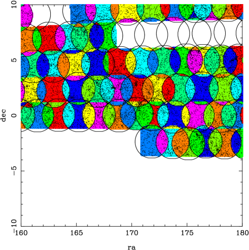
Both the recent 2dF galaxy redshift (2dFGRS) and the ongoing Sloan Digital Sky Survey (SDSS) adopted an adaptive tiling system in order to target photometrically selected galaxies for spectroscopic follow-up. The circular tiles within which spectra could be taken in a single pointing of the telescope were adaptively fitted over the survey region, with regions of high galaxy density being covered by two or more tiles. A region of such tiling is shown in Fig. 6. This procedure divides the survey into segments, each with a different completeness - the ratio of good quality spectra to galaxies targeted. It is usually assumed that this completeness is uniform across each of the segments formed by overlapping tiles. Understanding this completeness is a major consideration when performing a large-scale structure analysis of either of these surveys. Note that the distribution of segments depends on all adjoining targeted tiles, not just those that have been observed.

As well as understanding the completeness, we also need to consider the effect of the weather - spectra taken under bad observing conditions will tend to preferentially give redshifts for nearby rather than distant galaxies. We also need to worry about bad fields - regions near bright stars where photometric data is of poor quality. For the SDSS, there are hard limits for the spectroscopic region depending on how much photometric data was available when the targeting algorithm was run. All of these effects are well known and can be included in an analysis.

7.3 radial distribution

Figure 7: Redshift distribution of spectroscopically observed galaxies within the SDSS DR4 with apparent R magnitude less than $17.5$ and $17.77$ (solid circles). For comparison we show the best fit model given by Eq. 44 for each distribution (solid lines).

In addition to the angular distribution of galaxies, we also need to be able to model the radial distribution – in the formalism introduced in Section 6.2, we need this information in order to create the random catalogue. Perhaps the best way of doing this is to model the true luminosity function of the distribution of observed galaxies, and then apply a magnitude cut-off. This was the procedure adopted in cole05 . However, the reduction in the amplitude of the recovered power spectrum caused by fitting to the redshift distribution is small and it is common to simply fit a functional form to the distribution. In Fig. 7 we present the distribution of galaxy redshifts in the SDSS DR4 sample compared with a fit of the form baugh93

$$f(z)=z^{g}\exp\left[-\left(\frac{z}{z_{c}}\right)^{b}\right],$$ (44)

where $g$, $b$ and $z_{c}$ are free parameters that have been fitted to the data.

8 results from recent surveys

8.1 results

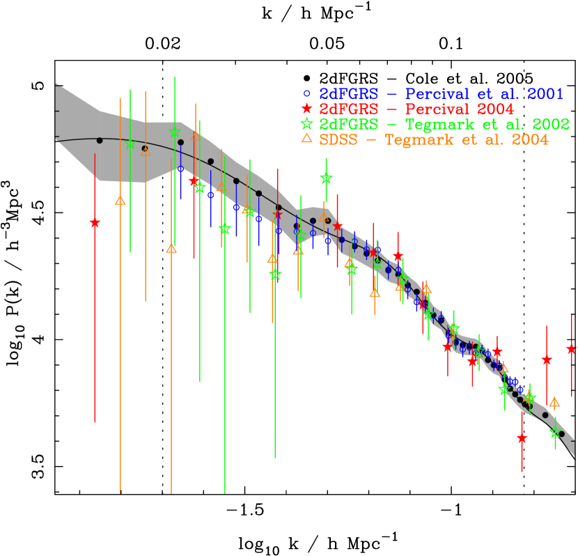
In Table 1 we summarise recent cosmological constraints derived from the 2dFGRS and SDSS. In order to provide a fair test of different analyses, we have only presented best-fit parameters and errors for $\Omega_{M}h$, fixing the other important parameters. Degeneracies between parameters, caused by the similarity between power spectrum shapes shown in Fig. 1 mean that, it is only the most recent analyses of the largest samples that can simultaneously constrain 2 or more of these parameters. In Table 1 we also presented the number of galaxy redshifts used in each analysis.

Table 1: Summary of recent cosmological constraints from 2dFGRS and SDSS galaxy redshift surveys. To try to provide a fair comparison, we only present the best-fit value and quoted error for $\Omega_{M}h$ assuming that all other cosmological parameters are fixed ($n_{s}=1$, $h=0.72$, $\Omega_{b}/\Omega_{M}=0.17$, $\Omega_{\nu}/\Omega_{M}=0.0$), and marginalise over the normalisation.

survey	reference	galaxy redshifts	method	$\Omega_{M}h$
2dFGRS	percival01	166490	Fourier	$0.206\pm 0.023$
2dFGRS	percival04	142756	Spherical Harmonics	$0.215\pm 0.035$
2dFGRS	cole05	221414	Fourier	$0.172\pm 0.014$
SDSS	pope04	205484	KL analysis	$0.207\pm 0.030$
SDSS	tegmark04	205443	Spherical Harmonics	$0.225\pm 0.040$
SDSS LRG	eisenstein05	46748	correlation function	$0.185\pm 0.015$

The power spectra recovered from these analyses are compared in Fig. 8. We have corrected each for survey window function effects using the best-fit model power spectrum. The amplitudes have also been matched, so this plot merely shows the shapes of the spectra. It is clear that the general shape of the galaxy power spectrum is now well known, and the turn-over is detected at high significance. The exact position of the turn-over is however, more poorly known and by examining the final column of Table 1, we see that there are discrepancies between recent analyses at the $\sim 2\sigma$ level.

Figure 8: Plot comparing galaxy power spectra calculated by different analysis techniques for different surveys. The redshift-space power spectrum calculated by cole05 (solid circles with 1-$\sigma$ errors shown by the shaded region) are compared with other measurements of the 2dFGRS power spectrum shape by percival01 – open circles, percival04 – solid stars, tegmark02 – open stars. Where appropriate the data have been corrected to remove effects of the survey volume, by calculating the effect on a model power spectrum with $\Omega_{M}h=0.168$, $\Omega_{b}/\Omega_{M}=0.0$, $h=0.72$ & $n_{s}=1$. A zero-baryon model was chosen in order to avoid adding features into the power spectra. All of the data are renormalized to match the power spectrum of cole05 . The open triangles show the uncorrelated SDSS real space $P(k)$ estimate of tegmark04 , calculated using their ‘modeling method’ with no FOG compression (their Table 3). These data have been corrected for the SDSS window as described above for the 2dFGRS data. The solid line shows a model linear power spectrum with $\Omega_{M}h=0.168$, $\Omega_{b}/\Omega_{M}=0.17$, $h=0.72$, $n_{s}=1$ and normalization matched to the 2dFGRS power spectrum.

9 combination with CMB data

In this section we consider recent CMB observations and see how the complementarity between CMB and large scale structure constraints can break degeneracies inherent in these data. The major steps required in a joint analysis are described, leading up to Section 9.5, in which we present the constraints from an example fit to recent data.

9.1 cosmological models

Before we start looking at constraining cosmological models using CMB and galaxy $P(k)$ data, it is worth briefly introducing the set of commonly used cosmological parameters (for further discussion see the recent review by lahav06 ). It is standard to assume Gaussian, adiabatic fluctuations, and we will not discuss alternatives here. It is possible to parameterise the cosmological model using a number of related sets of parameters. It is vital in any analysis that the model that is being fitted to the data is fully specified – including parameters and assumed priors. Many parameters have values that simplify the theory from which the models are calculated (e.g. the assumption that the total density in the Universe is equal to the critical density). Whether the data justify dropping one of these assumptions is an interesting Bayesian question liddle04 , which is outside the remit of the overview presented here, and we will simply introduce the parameters commonly used and possible assumptions about their values.

First, we need to know the geometry of the Universe, parameterised by total energy density $\Omega_{\rm tot}$, or the curvature $\Omega_{K}$, with the “simplified” value being that the energy density is equal to the critical value ($\Omega_{\rm tot}=1$, $\Omega_{K}=0$). We also need to know the constituents of the energy density, which we parameterise by the dark matter density $\Omega_{c}$ , baryon density $\Omega_{b}$, and neutrino density $\Omega_{\nu}$. Although it is commonly assumed that the combined neutrinos mass has negligible cosmological effect. The combined matter density $\Omega_{M}=\Omega_{c}+\Omega_{b}+\Omega_{\nu}$ could also be defined as a parameter, replacing one of the other density measurements. We also need to specify the dark energy properties, particularly the equation of state $w(a)$, which is commonly assumed to be constant $w(a)=-1$, so this field is equivalent to $\Lambda$. The perturbations after inflation are specified by the scalar spectral index $n_{s}$, with $n_{s}=1$ being the most simple assumption. Possible running of this spectral index is parameterised by $\alpha=dn_{s}/dk$ if included. A possible tensor contribution parameterised by the tensor spectral index $n_{t}$, and tensor-to-scalar ratio $r$ is sometimes explicitly included. The evolution to present day is parameterised by the Hubble constant $h$, and for the CMB the optical depth to last-scattering surface $\tau$. Finally, three parameters that are often ignored and marginalised over are the galaxy bias $b(k)$ (often assumed to be constant) and the CMB beam $B$ and calibration $C$ errors.

9.2 the MCMC technique

Large multi-parameter likelihood calculations are computationally expensive using grid-based techniques. Consequently, the Markov-Chain Monte-Carlo (MCMC) technique is commonly used for such analyses. While there is publically available code to calculate cosmological model constraints lewis02 , the basic method is extremely simple and relatively straightforward to code.

The MCMC method provides a mechanism to generate a random sequence of parameter values whose distribution matches the posterior probability distribution of a Bayesian analysis. Chains are sequentially calculated using the Metropolis algorithm metropolis53 : given a chain at position $x$, a candidate point $x^{\prime}$ is chosen at random from a proposal distribution $f(\mbox{\boldmath$x^{\prime}$}|\mbox{\boldmath$x$})$. This point is always accepted, and the chain moves to point $x^{\prime}$, if the new position has a higher likelihood. If the new position $x^{\prime}$ is less likely than $x$, then $x^{\prime}$ is accepted, and the chain moves to point $x^{\prime}$ with probability given by the ratio of the likelihood of $x^{\prime}$ and the likelihood of $x$. In the limit of an infinite number of steps, the chains will reach a converged distribution where the distribution of chain links are representative of the likelihood hyper-surface, given any symmetric proposal distribution $f(\mbox{\boldmath$x^{\prime}$}|\mbox{\boldmath$x$})=f(\mbox{\boldmath$x$}|\mbox{\boldmath$x^{\prime}$})$ (the Ergodic theorem: see, for example, roberts96 ).

It is common to implement dynamic optimisation of the sampling of the likelihood surface (see gilks96 for examples). Again, it is simple to assume a multi-variate Gaussian proposal function, centered on the current chain position. Given such a proposal distribution, and an estimate of the covariance matrix for the likelihood surface at each step, the optimal approach for a Gaussian likelihood would proceed as follows.

Along each principal direction corresponding to an eigenvector of the covariance matrix, the variance $\sigma^{2}$ of the multi-variate Gaussian proposal function should be set to be a fixed multiple of the corresponding eigenvalue of the covariance matrix. To see the reasoning behind this, consider translating from the original 17 parameters to the set of parameters given by the decomposition along the principal directions of the covariance matrix each divided by the standard deviation in that direction. In this basis, the likelihood function is isotropic and the parameters are uncorrelated. Clearly an optimized proposal function will be the same in each direction, and we have adjusted the proposal function to have precisely this property. There is just a single parameter left to optimize – we are free to multiply the width of the proposal function by a constant in all directions. But we know that the optimal fraction of candidate positions that are accepted should be $\sim 0.25$ gelman96 , so we can adjust the normalization of the proposal width to give this acceptance fraction. Note that the dynamic changing of the proposal function width violates the symmetry of the proposal distribution $f(\mbox{\boldmath$x^{\prime}$}|\mbox{\boldmath$x$})$ assumed in the Metropolis algorithm. However, this is not a problem if we only use sections of the chains where variations between estimates of the covariance matrix are small.

The remaining issue is convergence – how do we know when we have sufficiently long chains that we have adequately sampled the posterior probability. A number of tests are available gelman92 ; verde03 , although it’s always a good idea to perform a number of sanity checks as well – for example, do we get the same result from different chains started a widely separated locations in parameter space?

9.3 introduction to the CMB

Figure 9: Plot comparing large scale structure (lower panel) and CMB (upper panel) power spectra. The angular CMB power spectrum was converted to comoving scales using the comoving distance to the last scattering surface. The matter power spectrum (solid – linear, dashed – non-linear, present day), has been ratioed to a smooth model with zero baryons in order to highlight the baryonic features. Dotted lines show the positions of the peaks in the CMB spectrum.

Over the past few years there has been a dramatic improvement in the resolution and accuracy of measurements of fluctuations in the temperature of the CMB radiation. The discovery of features, in particular, the first acoustic peak, in the power spectrum of the CMB temperature has led to a new data-rich era in cosmology debernardis00 ; hanany00 . More recently a significant leap forward was made with the release of the first year data from the WMAP satellite bennett03 ; hinshaw03 . The relative positions and heights of the acoustic peaks encode information about the values of the fundamental cosmological parameters, as discussed for the matter power spectrum in Section 4. For a flat cosmological model with $n_{s}=1$, $\Omega_{M}=0.3$, $h=0.7$ and $\Omega_{b}h^{2}=0.02$ the CMB and matter power spectra are compared in Fig. 9. In order to create Fig. 9, the angular CMB power spectrum was converted to comoving scales by considering the comoving scale of the fluctuations at the last scattering surface. In Fig. 9, the matter power spectrum has been ratioed to a smooth zero baryon model in in order to highlight features – even so, the baryon oscillations are significantly more visible in the CMB fluctuation spectrum. The vertical dotted lines in this plot are located at the peaks in the CMB spectrum and highlight the phase offset between the two spectra. The CMB peaks are $\pi/2$ out of phase with the matter peaks because they occur where the velocity is maximum, rather than the density at the last scattering surface – this is known as the velocity overshoot. Additionally there is a projection effect – the observed CMB spectrum is the 2D projection of 3D fluctuations, and so is convolved with an asymmetric function: the projection can increase, but not decrease the wavelength of a given fluctuation.

Figure 10: Upper panel: The 1-yr WMAP TT power spectrum (black circles) is plotted with the CBI (red triangles), VSA (green squares) and ACBAR (blue stars) data at higher $l$. Lower panel: The 1-yr WMAP TE power spectrum (black circles). In both panels the solid black line shows the best fit model calculated from fitting the CMB data.

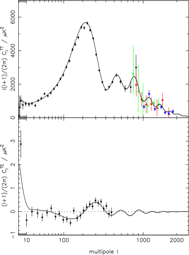
A compilation of recent CMB data is presented in Fig. 10. Here we have plotted both the temperature-temperature (TT) auto-power spectrum and the temperature-E-mode polarisation (TE) cross-power spectrum. The most significant current data set is, of course, the WMAP data shown by the solid circles in this figure. However, additional information is provided on small scales by a number of other experiments. In Fig. 10, we plot data from the CBI cbi , VSA vsa , and ACBAR acbar experiments.

Figure 11: 2D projections of the 7D likelihood surface resulting from a fit to the CMB data plotted in Fig. 10. The shading represents areas with $-2\Delta{\cal L}=2.3,6.0,9.2$ corresponding to $1\sigma$, $2\sigma$ and $3\sigma$ confidence intervals for multi-parameter Gaussian random variables. There are two primary degeneracies - between $\Omega_{c}h^{2}$ and $h$ and between $n_{s}$, $\tau$ and $\Omega_{b}h^{2}$, which are discussed further in Section 9.4.

Likelihood surfaces from a multi-parameter fit to these CMB data are shown in Fig. 11. For this fit, 7 parameters were allowed to vary: $\Omega_{c}h^{2}$, $\Omega_{b}h^{2}$, $h$, $\tau$, $n_{s}$, $\sigma_{8}$, and $\Omega_{\nu}h^{2}$. Other cosmological parameters were set at their “model simplification” values as discussed in Section 9.1. In particular, we have assumed a flat cosmological model with $\Omega_{\rm tot}=1$ and that the tensor contribution to the CMB is negligible. In choosing this set of $7$ parameters, and using the standard MCMC technique we have implicitly assumed uniform priors for each. The constraints on the 7 fitted parameters are given in Table 2.

Table 2: Summary of cosmological parameter constraints calculated by fitting a 7-parameter cosmological model to the CMB data plotted in Fig. 10 and to the combination of these data with the measurement of the 2dFGRS power spectrum cole05 – see text for details. Data are given with $1\sigma$ error, except for $\Omega_{\nu}h^{2}$ which is presented as a 1$\sigma$ upper limit.

parameter	CMB constraint	CMB+2dFGRS constraint
$\Omega_{c}h^{2}$	$0.107\pm 0.015$	$0.106\pm 0.006$
$\Omega_{b}h^{2}$	$0.0238\pm 0.0021$	$0.0235\pm 0.00166$
$h$	$0.725\pm 0.096$	$0.718\pm 0.036$
$\tau$	$<0.204\pm 0.117$	$<0.195\pm 0.085$
$n_{s}$	$1.00\pm 0.064$	$0.987\pm 0.046$
$\sigma_{8}$	$0.703\pm 0.125$	$0.696\pm 0.085$
$\Omega_{\nu}h^{2}$	$<0.00700$	$<0.006$

9.4 parameter degeneracies in the CMB data

Figure 12: As Fig. 10, but now showing 3 different models: the dashed line shows the best fit model in all panels – the model plotted in Fig. 10. The solid lines in the top-left panel were calculated with $h=\pm 0.1$, top-right $\Omega_{c}\pm 0.1$, bottom-left $\tau+0.3$ and $\tau=0$, and bottom-right $n_{s}\pm 0.2$.

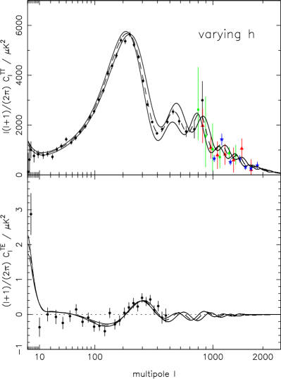
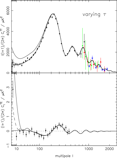
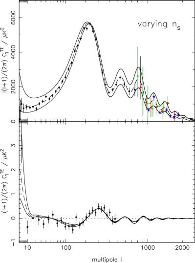
By examining Fig. 11 we see that the CMB data alone do not constrain all of the fundamental cosmological parameters considered to high precision. Degeneracies exist between certain combinations of parameters which lead to CMB fluctuation spectra that cannot be distinguished by current data efstathiou99 . To help to explain how these degeneracies arise, CMB models with different cosmological parameters are plotted in Fig. 12.

Constraining models to be flat does not fully break the geometrical degeneracy present when considering models with varying $\Omega_{\rm tot}$, and a degeneracy between the dark matter density $\Omega_{c}$ and the Hubble parameter $h$ remains. Fig. 12 shows that both $\Omega_{c}$ and $h$ affect the location of the first acoustic peak. A simple argument can be used to show that models with the same value of $\Omega_{m}h^{3.4}$ predict the same apparent angle subtended by the light horizon and therefore the same location for the first acoustic peak in the TT power spectrum percival02 . The degeneracy in Fig. 11 roughly follows this prediction.

There is another degeneracy that that can be seen in Fig. 11 between $n_{s}$, $\tau$ and $\Omega_{b}h^{2}$. From Fig. 12, we see that the effect of the optical depth $\tau$ on the shape of the TT power spectrum occurs predominantly at low multipoles. By adjusting the tilt of the primordial spectrum ($n_{s}$), the low-$\ell$ power spectrum can be approximately corrected for the change in $\tau$, and the high-$\ell$ end can be adjusted by changing the baryon density. This degeneracy is weakly broken by the TE data which provide an additional constraint on $\tau$.

9.5 results from the combination of LSS and CMB data

The CMB degeneracy between $\Omega_{c}$ and $h$ can be broken by including additional constraints from the power spectrum of galaxy clustering. There have been a number of studies using both CMB and large-scale structure data to set cosmological constraints, with a seminal paper coming from the WMAP collaboration spergel03 . Recently new small-scale CMB data and large-scale structure analyses have increased the accuracy to which the cosmological parameters are known. tegmark04b ; sanchez06 .

Figure 13: As Fig 11, but now including extra constraints from the 2dFGRS analysis of cole05 . These constraints helps to break the primary degeneracies discussed in Section 9.4.

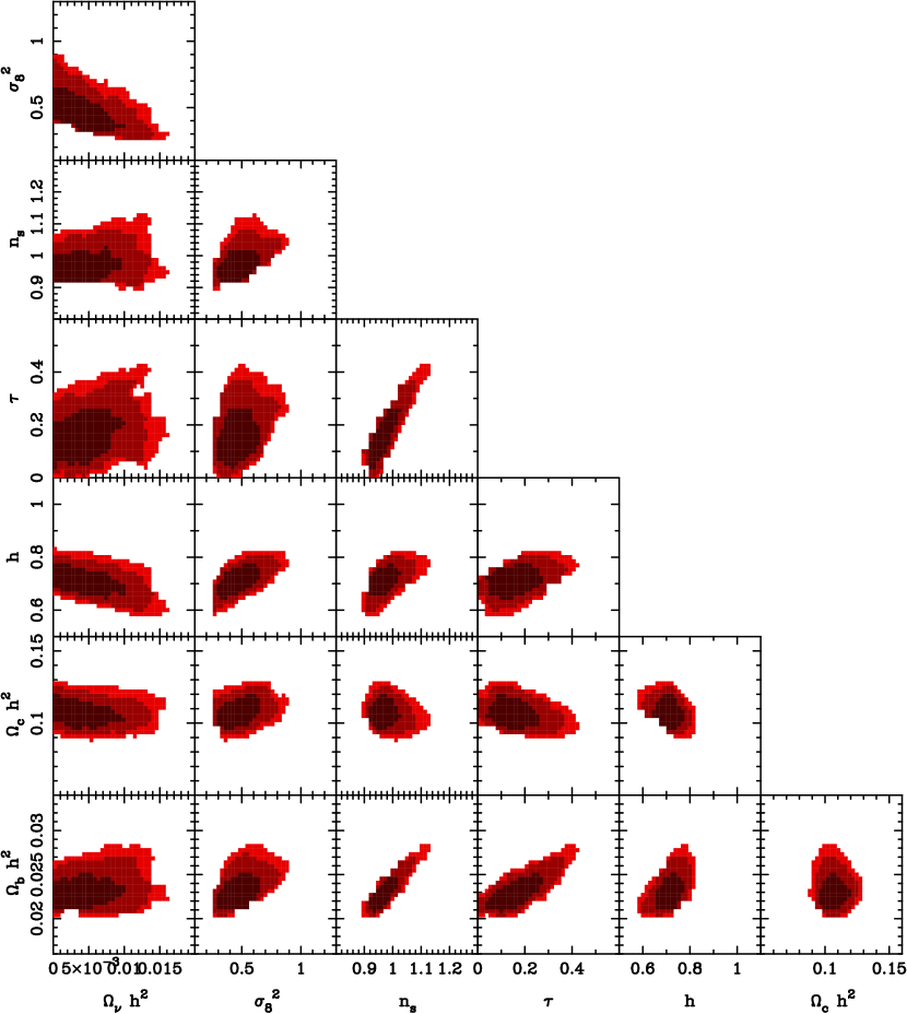
In Fig. 13, we provide a likelihood plot as in Fig 11, but now including the cosmological constraints from the final 2dFGRS power spectrum cole05 . For this analysis, a constant bias was assumed and we fitted the galaxy power spectrum over the range $0.02<k<0.15\,h\,{\rm Mpc}^{-1}$. The derived parameter constraints for the 7 parameters varied are compared with the constraints from fitting the CMB data only in Table 2. The physical neutrino density $\Omega_{\nu}h^{2}$ is unconstrained within the prior interval (physically, it must be $>0$), so we only provide an upper limit.

A Table of parameter constraints, such as that presented in Table 2 represents the end point of our story. We have introduced the major steps required to utilise a galaxy survey to provide cosmological parameter constraints, and have ended up with an example of a set of constraints for a particular model.

References

- (1) Adelman-McCarthy J.K., et al., 2005, astro-ph/0507711
- (2) Bashinsky S., Bertschinger E., 2001, Phys.Rev.Lett., 87, 081301
- (3) Bashinsky S., Bertschinger E., 2002, Phys.Rev.D, 65, 123008
- (4) Baugh C., Efstathiou G., 1993, MNRAS, 265, 145
- (5) Baumgart D.J., Fry J.N., 1991, ApJ, 375, 25
- (6) Bennett C.L., et al., 2003, ApJS, 148, 1
- (7) de Bernardis P., et al., 2000, Nature, 404, 955
- (8) Birkhoff G., 1923, Relativity and Modern Physics, Harvard University Press, Cambridge, Mass.
- (9) Cole S., Kaiser N., 1989, MNRAS, 237, 1127
- (10) Cole S., et al., 2005, MNRAS, 362, 505
- (11) Coles P., Lucchin F., 1995, Cosmology, The Origin and Evolution of Cosmic Structure, Wiley
- (12) Colless M., et al., 2003, astro-ph/0306581
- (13) Cooray A., Sheth, R., 2002, Physics Reports, 372, 1
- (14) Dickinson C., et al., 2004, MNRAS, 353, 732
- (15) Dodelson S., 2003, Modern Cosmology, Academic Press
- (16) Efstathiou G., Bond J.R., 1999, MNRAS, 304, 75
- (17) Eisenstein D.J., Hu W., 1998, ApJ, 496, 605
- (18) Eisenstein D.J., et al., 2001, AJ, 122, 2267
- (19) Eisenstein D.J., et al., 2005, ApJ, 633, 560
- (20) Fisher K.B., Scharf C.A., Lahav O., 1994, MNRAS, 266, 219
- (21) Feldman H.A., Kaiser N., Peacock J.A., 1994, MNRAS, 426, 23
- (22) Gelman A., Rubin D., 1992, Statistical Science 7. 457
- (23) Gelman A., Roberts G.O, Gilks W.R., 1996, in eds Bernardo J.M., Berger J.O., Dawid A., Smith A., Bayesian Statistics 5, 599, OUP
- (24) Gilks W.R., Richardson S., Spiegelhalter D.J., Markov chain monte carlo in practice, 1996, Chapman & Hall
- (25) Hamilton A.J.S., 2005, “Data analysis in Cosmology”, ed. V.Matrinez, Springer-Verlag lecture notes in Physics, astro-ph/0503603
- (26) Hamilton A.J.S., 2005, “Data analysis in Cosmology”, ed. V.Matrinez, Springer-Verlag lecture notes in Physics, astro-ph/0503604
- (27) Hanany S., et al., 2000, ApJ, 545, L5.
- (28) Hawkins E., et al., 2003, MNRAS, 346, 78
- (29) Heavens A.F., Taylor A.N., 1995, MNRAS, 275, 483
- (30) Hinshaw G., et al., 2003, ApJS, 148, 135
- (31) Kaiser N., 1987, MNRAS, 227, 1
- (32) Kuo C.L., et al., 2004, ApJ, 600, 32
- (33) Lahav O., Liddle A.R., 2006, Phys. Lett. B 592, 1 (2004) and 2005 partial update for the 2006 edition available at the PDG WWW pages at http://pdg.lbl.gov/, astro-ph/0601168
- (34) Landy S.D., Szalay A.S., 1993, ApJ, 412, 64
- (35) Lewis A., Bridle S., 2002, Phys. Rev. D, 66, 103511
- (36) Liddle A.R., Lyth D.H., Physics Reports, 231, 1, astro-ph/9303019
- (37) Liddle A.R., Lyth D.H., 2000, Cosmological Inflation and Large-Scale Structure, Cambridge University Press
- (38) Liddle A.R., 2004, MNRAS, 351, L49
- (39) Metropolis N., Rosenbluth A.W., Rosenbluth M.N., Teller A.H., Teller E., 1953, Journal of Chemical Physics, 21, 1087
- (40) Mo H.J., White S.D.M., 1996, MNRAS, 282, 347
- (41) Peacock J.A., 1999, Cosmological Physics, Cambridge University Press
- (42) Peacock J.A., Smith R.E., 2000, MNRAS, 318, 1144
- (43) Percival W.J., et al., 2001, MNRAS, 327, 1297
- (44) Percival W.J., et al., 2002, MNRAS, 337, 1068
- (45) Percival W.J., Verde L., Peacock J.A., 2004, MNRAS, 347, 645
- (46) Percival W.J., et al., 2004, MNRAS, 353, 1201
- (47) Percival W.J., 2005, A&A, 443, 819
- (48) Peebles P.J.E., 1973, ApJS, 185, 413
- (49) Pope A.C., et al., 2004, ApJ, 607, 655
- (50) Readhead A.C.S., et al., 2004, ApJ, 609, 498
- (51) Roberts G.O., 1996, in eds Gilks W.R., Richardson S., Spiegelhalter D.J., Markov chain monte carlo in practice, Chapman & Hall
- (52) Sanchez A.G., et al., 2006, MNRAS accepted, astro-ph/0507583
- (53) Seaborne M.D., et al., 1999, MNRAS, 309, 89
- (54) Seljak U., 2000, MNRAS, 318, 203
- (55) Sheth R.K., Tormen G., 1999, MNRAS, 308, 119
- (56) Smith R.E., et al., 2003, MNRAS, 341, 1311
- (57) Spergel D.N., et al., 2003, ApJS, 148, 175
- (58) Tadros H., et al., 1999, MNRAS, 305, 527
- (59) Tegmark M., Hamilton A.J.S., Xu Y., 2002, MNRAS, 335, 887
- (60) Tegmark M., et al., 2004, ApJ, 606, 702
- (61) Tegmark M. et al., 2004b, Phys. Rev. D, 69, 103501
- (62) Verde L., et al., 2003, ApJS, 148, 195
- (63) Wang L., Steidhardt P.J., 1998, ApJ, 508, 483
- (64) Wild, V., et al, 2005, MNRAS, 356, 247