A multifrequency angular power spectrum analysis of the Leiden polarization surveys

The Galactic synchrotron emission is expected to be the most relevant source of astrophysical contamination in cosmic microwave background polarization measurements, at least at frequencies $\nu\,\lower 2.0pt\hbox{${<\atop\hbox{\raise 4.0pt\hbox{$\sim$}}}$}\,70$ GHz and at angular scales $\theta\,\lower 2.0pt\hbox{${>\atop\hbox{\raise 4.0pt\hbox{$\sim$}}}$}\,30^{\prime}$. We present a multifrequency analysis of the Leiden surveys, linear polarization surveys covering the Northern Celestial Hemisphere at five frequencies between 408 MHz and 1411 MHz. By implementing specific interpolation methods to deal with these irregularly sampled data, we produced maps of the polarized diffuse Galactic radio emission with a pixel size $\simeq 0.92^{\circ}$. We derived the angular power spectrum (APS) ($PI$, $E$, and $B$ modes) of the synchrotron dominated radio emission as function of the multipole, $\ell$. We considered the whole covered region and some patches at different Galactic latitudes. By fitting the APS in terms of power laws ($C_{\ell}\sim\kappa\cdot\ell^{\alpha}$), we found spectral indices that steepen with increasing frequency: from $\alpha\sim-$(1-1.5) at 408 MHz to $\alpha\sim-$(2-3) at 1411 MHz for $10\,\lower 2.0pt\hbox{${<\atop\hbox{\raise 4.0pt\hbox{$\sim$}}}$}\,\ell\,\lower 2.0pt\hbox{${<\atop\hbox{\raise 4.0pt\hbox{$\sim$}}}$}\,100$ and from $\alpha\sim-0.7$ to $\alpha\sim-1.5$ for lower multipoles (the exact values depending on the considered sky region and polarization mode). The bulk of this flattening at lower frequencies can be interpreted in terms of Faraday depolarization effects. We then considered the APS at various fixed multipoles and its frequency dependence. Using the APSs of the Leiden surveys at 820 MHz and 1411 MHz, we determined possible ranges for the rotation measure, $RM$, in the simple case of an interstellar medium slab model. Also taking into account the polarization degree at 1.4 GHz, it is possible to break the degeneracy between the identified $RM$ intervals. The most reasonable of them turned out to be $RM\sim 9-17$ rad/m² although, given the uncertainty on the measured polarization degree, $RM$ values in the interval $\sim 53-59$ rad/m² cannot be excluded.

1 Introduction

In the last decade an impressive number of experiments has been dedicated to measurements of the cosmic microwave background (CMB) anisotropies, first observed in temperature by COBE (Smoot et al. (1990)). Modern cosmologies predict also the existence of polarization fluctuations, produced at the recombination epoch via Thomson scattering (see, e.g., Kosowski (1999)). However, the foreseen degree of polarization of the CMB anisotropies should be $\,\lower 2.0pt\hbox{${<\atop\hbox{\raise 4.0pt\hbox{$\sim$}}}$}\,10\%$, implying a signal much weaker than in temperature and therefore extremely difficult to reveal. The first detection of the CMB polarization achieved by DASI (Kovac (2002)) and the recent measure by BOOMERanG (Masi et al. (2005); Montroy et al. (2005)) confirmed the expectations. The polarization data expected by the NASA WMAP  satellite will permit us to extend the information about polarization to a wider portion of the sky, though at small scales ($\theta\,\lower 2.0pt\hbox{${<\atop\hbox{\raise 4.0pt\hbox{$\sim$}}}$}\,0.5^{\circ}$) its sensitivity will likely allow a detection rather than an accurate measure.

In the near future, the ESA Planck  satellite will significantly improve these results by observing the whole sky at nine different frequencies between 30 and 857 GHz, both in temperature and polarization, with unprecedented resolution and sensitivity (e.g. see Tauber (2004) and references therein). In particular, the sensitivities per pixel of the Planck maps are expected to be between 3-4 and 10 times better than in the WMAP data, producing a significant improvement in terms of angular power spectrum recovery. Consequently, Planck alone will allow an estimate of the cosmological parameters much more precise than that obtained by WMAP and other CMB experiments combined with different cosmological data. Moreover, it will accurately measure the CMB $E$-mode and could potentially observe the $B$-mode as well (e.g. see Burigana et al. (2004) and references therein).

Strong efforts have been made to evaluate the impact of the foregrounds on the feasibility of CMB anisotropy measurements, as well as to understand how to separate the different components contributing to the observed maps. The methods elaborated for this purpose can be divided in two categories: blind (Independent Component Analysis, see Baccigalupi et al. (2000); Maino et al. (2002); Baccigalupi et al. (2004); Delabrouille et al. (2003)) and non-blind (Wiener filtering and Maximum Entropy Methods, see respectively Bouchet et al. (1999) and Hobson et al. (1998)). The latter class needs an a priori knowledge of the frequency and spatial dependence of the foreground properties, while a blind approach only requires maps at different frequencies as input. On the other hand, blind methods benefit from having ancillary data (such as realistic templates) to improve the separation robustness and quality .

The Galactic polarized diffuse synchrotron radiation is expected to play a major role at frequencies below 70 GHz on intermediate and large angular scales ($\theta\,\lower 2.0pt\hbox{${>\atop\hbox{\raise 4.0pt\hbox{$\sim$}}}$}\,30^{\prime}$), at least at medium and high Galactic latitudes where satellites have the clearest view of the CMB anisotropies. At about 1 GHz the synchrotron emission is the most important radiative mechanism out of the Galactic plane, while at low latitudes it is comparable with the bremsstrahlung; however the free-free emission is unpolarized, whereas the synchrotron radiation could reach a theoretical intrinsic degree of polarization of about $75\%$. Consequently, radio frequencies are the natural range for studying the Galactic synchrotron emission, although it might be affected by Faraday rotation and depolarization. Nowadays the only available data suitable for studying the polarized Galactic synchrotron emission on large scales are the so-called Leiden surveys (Brouw & Spoelstra (1976)). These are linear polarization surveys, extending up to high Galactic latitudes, carried out at five frequencies between 408 MHz and 1411 MHz. We have elaborated specific interpolation methods to project these surveys into maps with a pixel size $\simeq 0.92^{\circ}$. These maps can be exploited in different contexts. They are suitable to analyse the statistical properties of the Galactic radio polarized emission. Beside this obvious application, they can be used as input to construct templates for simulation activities in the context of current and future microwave polarization anisotropy experiments. For example they can be utilized to build templates for straylight evaluation (see, e.g., Challinor et al. (2000); Burigana et al. (2001);  Barnes et al. (2003)) and for component separation analyses.

It is standard practice to characterize the CMB anisotropies in terms of the angular power spectrum  (APS) as a function of the multipole, $\ell$ (inversely proportional to the angular scale, $\ell\simeq{180}/{\theta(^{\circ})}$). The APS is an estimator related to the angular two-point correlation function of the fluctuations of a sky field (Peebles (1993)). The APS is not able to fully characterize the complexity of the intrinsically non-Gaussian Galactic emission. Nevertheless, it is of increasing use also in the study of the correlation properties of the Galactic foregrounds (see, e.g., Baccigalupi et al. (2001) for an application to the polarized radio emission). We stick to the commonly adopted approach and consider the APS of both the polarized intensity, $PI$, and the $E$ and $B$ modes  (see Kamionkowski et al. (1997) and Zaldarriaga (2001)).

In Sect. 2 we briefly summarize the properties of the Leiden surveys and of some selected areas relevant for the analysis at the smaller angular scales. In Sect. 3 we introduce the general criteria adopted to elaborate the class of our interpolation algorithms. The final, optimized version of the algorithm and the accuracy of the derived maps and APSs are described in Sect. 4. In Sect. 5 we present our results in terms of maps, APSs, and a parametric description of the APSs. A brief comparison with a preliminary version of the DRAO polarization survey (Wolleben et al. (2003); Wolleben (2005)) at 1.4 GHz is given in Sect. 6 in terms of APS. Sect. 7 is devoted to the multifrequency analysis of our results and to their interpretation in the context of an interstellar medium slab model. We summarize and discuss our main results in Sect. 8.

2 The Leiden surveys and selected areas

The so-called Leiden surveys are the final results of different observational campaigns carried out in the sixties with the 25-m radio telescope at Dwingeloo. The complete data sets as well as the observation reduction and calibration methods have been presented by Brouw & Spoelstra (1976). The observations were performed at 408, 465, 610, 820 and 1411 MHz with an angular resolution of $\theta_{HPBW}=2.3^{\circ},2.0^{\circ},1.5^{\circ},1.0^{\circ},0.6^{\circ}$, respectively. At each frequency, the observed positions are inhomogenously spread over the Northern Galactic Hemisphere and globally cover a sky fraction of about $\sim 50\%$. The errors, quoted for points observed at least twice, follow Gaussian distributions with mean values of $0.34,0.33,0.16,0.11$ and $0.06$ K from the lower to the higher frequency, respectively. The observations at the same position were taken at different azimuths, elevations, and days (the adopted scanning strategy being random in coordinates and time). A robust control and removal of the ground radiation contaminating the observations have been also performed. These properties imply a very low level of contamination from residual systematic effects, at least in comparison with the intrinsic survey sensitivities, and make these surveys a reference point (though insufficient by itself) for absolute calibration of radio data. As an example, the absolute calibration of the Effelsberg maps at 1.4 GHz has been performed using the Leiden survey at 1411 MHz (see Uyaniker et al. (1998) for a description of the procedure).

The main problem in the analysis of the Leiden surveys is their poor sampling across the sky; it is necessary to project them onto maps with pixel size of about $3.7^{\circ}$ (we use here the HEALPix scheme, see Górski et al. (2005)) to find at least one observation on each pixel of the observed region, that would limit the angular power spectrum recovery to $\ell\simeq 50$. On the other hand, for some sky areas the sampling is significantly better than the average, by a factor $\simeq 4$, and the maps appear filled even for a pixel size of $\sim 1.8^{\circ}$, allowing one to reach multipoles $\ell\simeq 100$. We identified three regions that permit one to investigate this multipole range at both low and middle/high Galactic latitudes: patch 1 [($110^{\circ}\leq l\leq 160^{\circ}$, $0^{\circ}\leq b\leq 20^{\circ}$)]; patch 2 [($5^{\circ}\leq l\leq 80^{\circ}$, $b\geq 50^{\circ}$) together with ($0^{\circ}\leq l\leq 5^{\circ}$, $b\geq 60^{\circ}$) and ($335^{\circ}\leq l\leq 360^{\circ}$, $b\geq 60^{\circ}$)]; patch 3 [($10^{\circ}\leq l\leq 80^{\circ}$, $b\geq 70^{\circ}$)].

We underline that in these patches the polarized signal and the corresponding signal-to-noise ratio are typically higher than the average; they are associated with the brightest structures of the polarized radio sky, i.e. the “Fan Region” (patch 1) and the “North Polar Spur” (patch 2 and 3). The “North Polar Spur” (NPS) has been extensively studied (see Salter (1983) and Egger & Aschenbach (1995)). The theories that better match the observations are all variants of the same model and interpret the NPS as the front shock of an evolved Supernova Remnant (SNR), whose distance should be $\sim 100\pm 20$ pc (inferred from starlight polarization, see Bingham (1967)). In contrast, the present knowledge of the “Fan Region” is much poorer. A rough estimate of its distance can be derived from purely geometrical considerations: it has such an extent on the sky that it must be located within (1-2)$\times 10^{2}$ pc from the Sun not to have an unrealistically large dimension. Wolleben et al. (2005) has recently proposed a different view of the “Fan Region”: from the distances of HII regions that they consider to be located in front of this structure and to depolarize its synchrotron emission, they claim that the “Fan Region” is indeed an enormous object extending up to the Perseus Arm, i.e. up to $\approx$ kpc distance.
Another common and remarkable characteristic of the selected areas is that the polarization vectors appear mostly aligned at the two higher frequencies of the Leiden surveys.

3 Map production algorithm and consistency tests

A simple method to project the Leiden surveys into HEALPix maps is to average the observations falling in each pixel. However, the maps of the polarized intensity ($PI$) and of the Stokes parameters ($Q$,$U$) produced in this way show discontinuities on scales $\theta\simeq\theta_{pixel}$. These discontinuities tend to add spurious power in the recovered APS, particularly at multipoles $\ell\sim 180/\theta_{pix}$. In order to smooth these discontinuities we implemented a “class” of specific “interpolation” algorithms to generate maps with $\theta_{pix}\sim 0.92^{\circ}$, for the whole sky region covered by the surveys. To each pixel is assigned a weighted average of the signal values falling in its neighbourhood, i.e. $\sum_{i}(p_{i}\cdot x_{i})/\sum p_{i}$ with $p_{i}=1/(\sigma_{i}^{2}\cdot d_{i}^{n})$, where $x_{i}$ and $\sigma_{i}$ are the signal and the error associated with the observation and $d_{i}$ its angular distance from the pixel centre. The radius within which the average is computed varies pixel by pixel and is selected according to the following guidelines: (i) to have enough observations (at least 3); (ii) to use only observations quite close to the considered pixel centre (less than a few degrees); (iii) to minimize the resulting average fractional change of the signal with the variation of the number of points and of the radius. The first two conditions imply that the interpolation is as local as possible and is performed using a reasonable number of data points. The third recipe is a convergency criterion.

In order to check the reliability of the method, we generated at each frequency several groups of $PI$, $Q$, and $U$ maps, each corresponding to a different choice of the distance power in the average weight ($1/(\sigma^{2}\cdot d^{n})$) for various pixel sizes (ranging between $3.7^{\circ}$ and $0.92^{\circ}$). A detailed description of the consistency tests together with preliminary results referring to a first version of the polarized intensity maps have been reported in La Porta (2001) and Burigana & La Porta (2002). In that work we produced simulated maps of white noise, expected to contamine the astrophysical signal contained in the maps, according to three different recipes. We compared the APS of the simulated noise and signal maps to identify the ranges of multipoles statistically relevant (i.e. where the signal is not masked by the noise) for various considered sky coverages. We found that the analysis of the survey full coverage provides a good estimate of the polarization APS for $\ell\sim[2,50]$, while the better sampled patches (characterized by a higher S/N ratio on average) allow us to investigate the multipole interval $\sim[30,100]$. We emphasize that the current APS analysis has a statistical meaning and cannot provide details on the local properties of the synchrotron emission.

4 Interpolation algorithm optimization and accuracy

In order to evaluate and optimize the signal reconstruction quality provided by our algorithm, we performed a final test. Starting from simulated polarization maps having known statistical properties, we created a table of data analogous to the Leiden survey ones and run our code to build $PI$, $Q$ and $U$ maps to be compared with the input skies. We focused on the 1411 MHz case, because this is the most seriously undersampled both in terms of number of observations per beam and of observed points. Therefore, the maps produced at this frequency are potentially most influenced by the interpolation method effects, particularly at multipoles larger than some tens. We assumed $C_{\ell}^{E}=C_{\ell}^{B}=C_{\ell}={\kappa}\cdot\ell\leavevmode\nobreak\ ^{\alpha}$, with values of the parameters ${\kappa}$ and ${\alpha}$ in agreement with the mean law obtained for the Galactic polarized synchrotron emission in our first analysis of the 1411 MHz survey (reported in Burigana & La Porta (2002)). For $\ell\sim[30,200]$ we adopted  $\kappa=1(K^{2})$ and $\alpha=-3$. Applying the HEALPix facility Synfast to these angular power spectra, we generated maps of $Q$ and $U$ with a pixel size of $\simeq 13.7^{\prime}$ and a beamwidth $\theta_{HPBW}=36^{\prime}$, as in the 1411 MHz survey, and used them to build the simulated table of data as described below.
At each observed position of the Leiden survey

• We first assigned the Stokes parameters corresponding to the Synfast simulation pixel in which it would project and

• The corresponding rms given in the original table.

• We then added to each Stokes parameter a random value extracted from a Gaussian distribution in order to mimic the effect of the instrumental white noise (see, e.g., Burigana & Sáez (2003)). The adopted standard deviation of this Gaussian distribution has been chosen equal to the mean error quoted for the considered original data. In this way the signal-to-noise ratio of the simulated table is statistically very close to the real case one.

We then obtained $PI$ as $\sqrt{Q^{2}+U^{2}}$ and calculated its error $\sigma_{PI}$ according to the standard error propagation rules.
Finally, we applied our interpolation method to the simulated data table and produced independently $PI$ ,$Q$, and $U$ simulated maps with $\theta_{pix}\simeq 0.92^{\circ}$. We ran our code several times, changing the weight $n$ to be adopted in the average and the criteria for selecting the interpolation radius, so to sort out the best solution.
As a first self-consistency test of the resulting maps, we verified that typically the $PI$ map can be considered equal to the $\sqrt{Q^{2}+U^{2}}$ within the uncertainty limit in $85\%$ of the pixels. Then we compared the reconstructed maps with the input sky maps directly obtained with the Synfast facility (see Fig. 1).

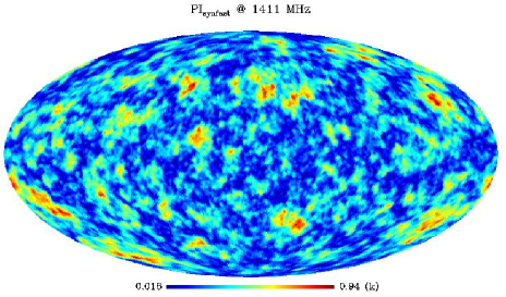
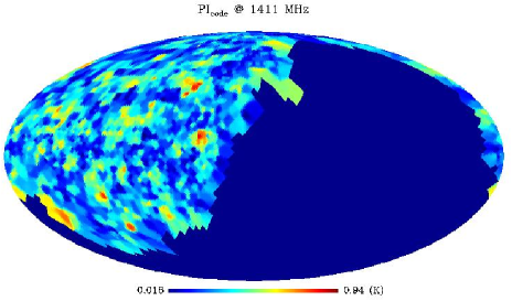
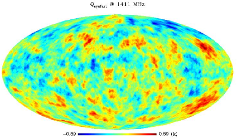
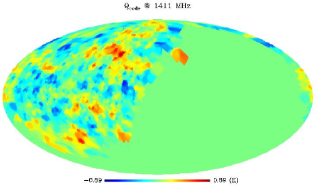
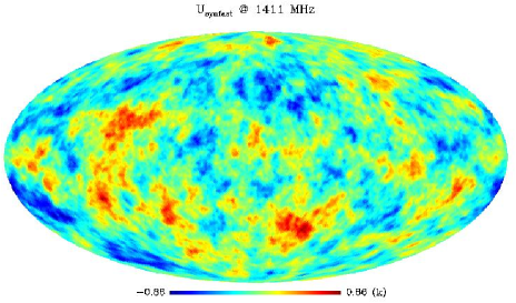
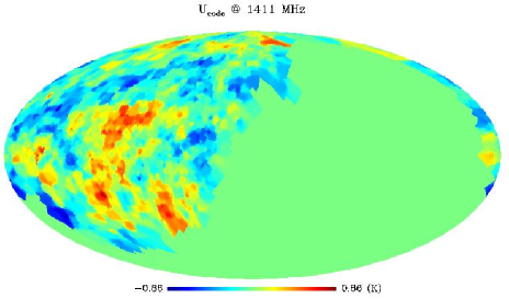
Figure 1: Synfast realizations (left side) at 1411 MHz versus maps reconstructed applying the final version of the filling code to the synthetic data table (right side). See text for details.

We first degraded  the Synfast simulations to $0.92^{\circ}$ pixel size maps and considered only the portion of the sky covered by the Leiden survey. Computing the APSs of both the original and the reprocessed maps we found that the best agreement between them is obtained:

1. Adopting as polarized intensity the quantity $\sqrt{Q_{reproc}^{2}+U_{reproc}^{2}}$ (instead of the $PI_{reproc}$, produced applying the filling code to the $PI$ values of the data table);

2. Using the weight $1/(\sigma^{2}\cdot d^{4})$; and

3. Interpolating the data in the minimum circle containing at least two observations.

The first choice is motivated by the necessity to (implicitly) preserve the information on the polarization angle and is a posteriori justified by the following result: the APS of $PI$ map reconstructed applying the code directly on the table of $PI$ values presents a certain loss in power with respect to the input case. The reason is likely that the $PI$ interpolated value overestimates the effective mean value of the field in the presence of changes in the signs of the Stokes parameters and consequently leads to an underestimation of the mean value of the field fluctuations.
Criteria 2 and 3 imply that the interpolation is as local as possible according to the sampling of each sky region. This approach is quite different from that pursued by other authors (Bruscoli et al. (2002)); they performed a Gaussian smoothing everywhere with constant $\theta_{HPBW}$ (of $3^{\circ}$), neglecting the sampling dependence on the position in the sky and on the frequency.
In principle, before computing any average we should have transformed the polarization vectors using the formula of the parallel transport on the sphere; however operating only a local interpolation, the consequent mixing of the two orthogonal components of the polarized signal turned out to be negligible .
Fig. 2 shows that the statistical information contained in the synthetic data table is appreciably traced out in the multipole ranges of interest both for the half-sky map and for the patches (for conciseness we report here only the results found for patch 2).

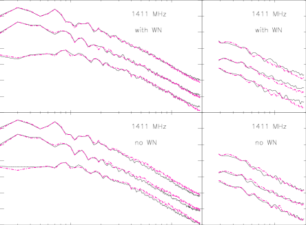
Figure 2: Comparison between the APSs of the input maps (dot lines) extracted from the Synfast simulations (degraded to $0.92^{\circ}$ pixel size maps) and the reprocessed maps (solid lines). From the bottom: $C_{\ell}^{PI}$, $C_{\ell}^{E}\cdot 10$ and $C_{\ell}^{B}\cdot 100$. Note the excellent agreement between the input and reprocessed APSs up to $\sim 100$.

Fitting the APS of the reprocessed map, we quantified the precision level at which the input values of the amplitude and of the spectral index were recovered: by considering several realizations for the various cases, we found relative errors within $\simeq 10\%$ for both the parameters.
We also checked the reliability of the maps themselves in a more quantitative way. The distributions of the pixel to pixel difference between the two series of maps (i.e. $PI$, $Q$ and $U$ produced by Synfast and reprocessed by our interpolation code) are, in all cases, close to Gaussian distributions, with standard deviations comparable with the typical mean error of the data table (see Table 1 and Fig. 3).

Half-sky	Gaussian interp.		distribution		% of pixels
	ave (mK)	rms (mk)	ave (mK)	rms (mk)	$1\sigma$	$2\sigma$	$3\sigma$
$\Delta PI$	3.6	88.3	3.9	102.2	71.8	94.7	99.0
$\Delta Q$	-2.4	97.1	-0.9	109.6	71.5	94.9	99.1
$\Delta U$	-5.6	93.5	-9.1	114.3	73.7	94.8	98.7
Patch 1	Gaussian interp.		distribution		% of pixels
	ave (mK)	rms (mk)	ave (mK)	rms (mk)	$1\sigma$	$2\sigma$	$3\sigma$
$\Delta$P	6.3	61.6	7.7	73.7	71.8	94.4	98.9
$\Delta$Q	-7.5	68.2	-8.2	76.2	70.8	95.4	99.2
$\Delta$U	-6.6	66.1	-6.8	77.4	72.1	94.4	99.1
Patch 2	Gaussian interp.		distribution		% of pixels
	ave (mK)	rms (mk)	ave (mK)	rms (mk)	$1\sigma$	$2\sigma$	$3\sigma$
$\Delta PI$	1.2	74.9	3.5	80.3	70.7	95.1	99.6
$\Delta Q$	1.6	81.1	-3.5	85.5	70.0	94.8	99.4
$\Delta U$	-3.2	75.0	-10.2	85.2	70.5	95.9	99.0
Patch 3	Gaussian interp.		distribution		% of pixels
	ave (mK)	rms (mk)	ave (mK)	rms (mk)	$1\sigma$	$2\sigma$	$3\sigma$
$\Delta PI$	6.0	72.8	1.4	78.9	69.4	96.3	99.7
$\Delta Q$	1.2	68.5	-3.4	71.9	69.0	94.6	99.7
$\Delta U$	-13.9	75.7	-13.9	81.0	68.0	94.6	99.3

Table 1: The pixel to pixel difference between the maps directly generated with Synfast (after degradation to $0.92^{\circ}$ pixel size maps) and the reconstructed maps contaminated by white noise, for the whole survey and the considered patches. Columns 2 and 3 give the average and rms of the Gaussian function that best fits the difference distribution (shown in Fig. 3). Columns 4 and 5 contain the average and standard deviation of the difference distribution. Columns 6, 7 and 8 give the percentages of pixels with absolute difference within the reported levels (here $1\sigma$ corresponds to the rms reported in column 5).

Figure 3: Distribution of the pixel to pixel differences between the maps directly simulated with Synfast (degraded to $0.92^{\circ}$ pixel size maps) and the reprocessed maps at 1411 MHz. We display here the results of the test, both with (upper panels) and without (lower panels) white noise contamination, in the case of the full coverage 1411 MHz Leiden survey. The superimposed curves are the Gaussian distributions giving the best fit to the data.

We repeated the test described above skipping the step c) . The distributions of the differences between the input and reprocessed maps are again close to Gaussian distributions, but with standard deviations slightly smaller than those found including step c) (in particular, for the full survey coverage the standard deviation is now smaller by about $20\%$). This indicates the existence of a geometric contribution in the error distribution over the maps related to the poor sampling of the data. Expressing the rms of the pixel to pixel difference distribution as

$$\sigma_{map}\simeq\sqrt{\sigma_{samp}^{2}+\sigma_{WN}^{2}}$$

the analysis of reprocessed maps (with and without noise) gives

$$\sigma_{WN}\simeq{\rm const}\times\sigma_{samp}$$

with ${\rm const}\simeq 0.63,0.87,0.90,1.15$, respectively for the whole survey coverage and for the patches 1, 2, and 3, without significant differences among the maps of $PI$, $Q$ or $U$.
The relative weight of the geometrical contribution to the overall error decreases with the goodness of the sampling. At the other frequencies of the Leiden surveys the sampling and the signal-to-noise ratio are better than at 1411 MHz; as a consequence, we can look at the ratio between $\sigma_{samp}$ (resp. $\sigma_{map}$) and the signal at 1411 MHz as a conservative upper limit to the relative error caused by geometric effects (resp. geometric effects plus experiment white noise) at the lower frequencies.

To verify whether the goodness of the signal reconstruction depends on the input sky characteristics, we repeated the entire test adopting a different input APS, more appropriate at 408 MHz. At this frequency the analysis of the preliminary polarization maps led to different results for the APSs than the 1411 MHz case. In particular, the spectral index was flatter (roughly $\sim-1.5$ in the multipole range [30,200]), both for the whole coverage map and for the patches. The same test repeated with this slope confirmed the results described before. The quality of the APS reconstruction is slightly less accurate than in the previous case, however the relative errors estimated for the recovered amplitudes and spectral indices remain within $\simeq 10\%$.

5 Results

In Fig. 4 we show the polarization maps ($PI$, $Q$, and $U$) produced at all frequencies with the final version of the code described in the previous section.

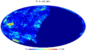
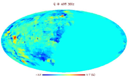
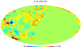
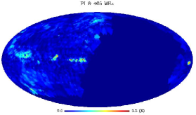
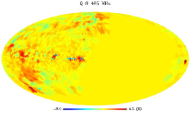
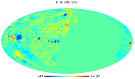
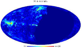
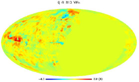
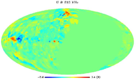
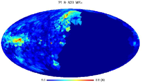
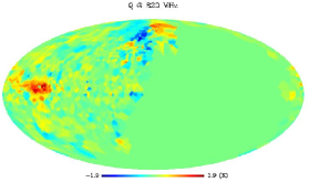
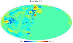
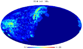
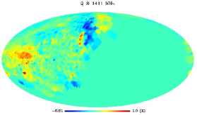
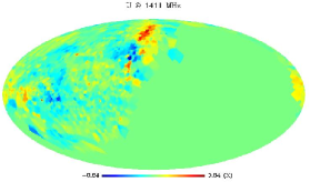
Figure 4: $PI$, $Q$, and $U$ maps obtained from the Leiden surveys data tables using the final version of the interpolation algorithm at all frequencies.

Using the Anafast facility of the HEALPix package, we computed the APSs of the polarized intensity and of the $E$ and $B$ modes for the half-sky coverage and for the patches  at the five frequencies of the surveys. In addition to the three better sampled areas we considered another region (patch 4) located at ($70^{\circ}\leq l\leq 120^{\circ}$, $-45^{\circ}\leq b\leq-15^{\circ}$). This patch has a sky sampling in the average (its APS is then statistically relevant only for $\ell\,\lower 2.0pt\hbox{${<\atop\hbox{\raise 4.0pt\hbox{$\sim$}}}$}\,50$) and is characterized by a rather low signal.

The $E$ and $B$ modes turned out to be extremely similar, so that, instead of studying each of them singularly, we consider their average $(C_{\ell}^{E}+C_{\ell}^{B})/2$. In some cases (namely for patch 1 and 2 at 1411 MHz and patch 2 and 4 at 408 MHz) we could even consider a unique APS defined as $(C_{\ell}^{PI}+C_{\ell}^{E}+C_{\ell}^{E})/3$.
The maps represent the Galactic polarized synchrotron emission, smoothed with the beam of the radiotelescope and contaminated by the noise. As a consequence, their APSs can be fit as sum of two components, $C_{\ell}=C_{\ell}^{synch}W_{\ell}+C_{\ell}^{\rm N}$. We exploit the power law approximation $C_{\ell}^{synch}\simeq\kappa\cdot\ell^{\leavevmode\nobreak\ \alpha}\,$ and assume a symmetric, Gaussian beam, i.e. a window function $W_{\ell}={\rm e}^{-(\sigma_{b}\ell)^{2}}$, where $\sigma_{b}={\theta_{HPBW}({\rm rad})/{\sqrt{8{\rm ln}2}}}$ . Under the hypothesis of uncorrelated Gaussian random noise  (white noise), $C_{\ell}^{\rm N}=C_{\ell}^{\rm WN}\sim$ const . We have performed the fit on the multipole range $[30,200]$ for the patches and $[2,200]$ for the full-coverage maps. In fact, the flattening occurring at higher multipoles helps recover the noise constant, in spite of the fact that no reliable astrophysical information can be derived for ${\ell}>100$ from the APSs even in the three better sampled regions (Burigana & La Porta (2002)). For the patches, we found that a single set of the parameters $\kappa$, $\alpha$ allows us to describe the APS in the entire range of multipoles. In the case of the survey full coverage we needed two sets of $\kappa$, $\alpha$, each of them appropriate to a certain multipole range. At all frequencies a change in the APS slope occurs corresponding to ${\ell}\sim 10$ for both $C_{\ell}^{PI}$ and $(C_{\ell}^{E}+C_{\ell}^{B})/2$.
As an example, we display in Fig. 5 the APS and the corresponding best fit curve at 610 MHz for the survey full coverage and one patch.

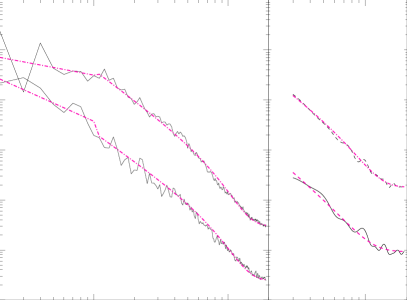
Figure 5: Polarization APSs at 610 MHz (solid lines) for the survey full coverage (left panel) and patch 3 (right panel) together with the corresponding best fit curves (dot-dash lines). The lower curves in each panel are $C_{\ell}^{PI}$, while the other ones represent $(C_{\ell}^{E}+C_{\ell}^{B})/2$ multiplied by 10.

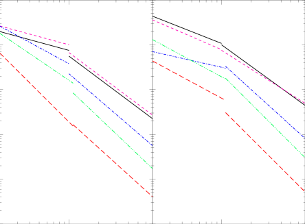
Figure 6: Synchrotron component of the APS derived for the survey full coverage for the polarized intensity (left panel) and for $(C_{\ell}^{E}+C_{\ell}^{B})/2$ (right panel) at the various frequencies: 408 (solid line), 465 (dashes), 610 (dot-dash), 820 (three dot-dash), and 1411 MHz (long dashes).

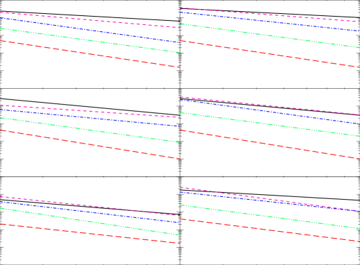
Figure 7: As in Fig. 6 but for the selected patches: patch 1 (top panels), patch 2 (middle panels), and patch 3 (bottom panels).

We show in Fig. 6 (resp. Fig 7) the recovered synchrotron term, $C_{\ell}^{synch}$, and list in Table 2 (resp. Table 3) the corresponding $\kappa$, $\alpha$ obtained for the survey full coverage (resp. for the patches). In the multipole range $30\,\lower 2.0pt\hbox{${<\atop\hbox{\raise 4.0pt\hbox{$\sim$}}}$}\,{\ell}\,\lower 2.0pt\hbox{${<\atop\hbox{\raise 4.0pt\hbox{$\sim$}}}$}\,100$ we found a general trend: from the lowest to the highest frequency the slope increases from $\sim-$(1-1.5) to $\sim-$(2-3), with a weak dependence on the considered sky region.

$\nu$	$C_{\ell}$	$\kappa_{1}$	$\alpha_{1}$	$\ell$	$\kappa_{2}$	$\alpha_{2}$
(MHz)	(mK2)	(mK2)			(mK2)
408	$EB$	$8.00\cdot 10^{4}$	-0.87	10.86	$4.00\cdot 10^{5}$	-1.60
	$PI$	$3.00\cdot 10^{4}$	-0.60	10.80	$2.50\cdot 10^{5}$	-1.65
465	$EB$	$7.00\cdot 10^{4}$	-0.95	10.00	$1.90\cdot 10^{5}$	-1.40
	$PI$	$4.00\cdot 10^{4}$	-0.60	10.85	$3.00\cdot 10^{5}$	-1.65
610	$EB$	$1.00\cdot 10^{4}$	-0.50	10.00	$4.00\cdot 10^{5}$	-2.00
	$PI$	$6.00\cdot 10^{4}$	-1.20	10.85	$1.8\cdot 10^{5}$	-1.90
820	$EB$	$3.00\cdot 10^{4}$	-1.19	11.00	$3.5\cdot 10^{5}$	-2.20
	$PI$	$5.10\cdot 10^{4}$	-1.50	11.00	$1.30\cdot 10^{5}$	-2.10
1411	$EB$	$1.00\cdot 10^{4}$	-1.19	11.00	$6.00\cdot 10^{4}$	-2.20
	$PI$	$3.00\cdot 10^{4}$	-2.20	11.00	$2.00\cdot 10^{4}$	-2.00

Table 2: Values of the best fit parameters $\kappa$ and $\alpha$ obtained in the analysis of the survey full coverage APS at all the frequencies (as shown in Fig.6). Relative errors on the best fit parameters are $\sim 10\%$. Two multipole ranges are considered: $[2,\ell]$ and $[\ell,200]$ ($\ell$ was also a free parameter in the fit). $EB$ refers to $(C_{\ell}^{E}+C_{\ell}^{B})/2$.

		408 MHz		465 MHz		610 MHz		820 MHz		1411 MHz
		$\kappa$ (mK2)	$\alpha$	$\kappa$ (mK2)	$\alpha$	$\kappa$ (mK2)	$\alpha$	$\kappa$ (mK2)	$\alpha$	$\kappa$ (mK2)	$\alpha$
P 1	$EB$	$9.80\cdot 10^{4}$	-0.99	$6.00\cdot 10^{5}$	-1.50	$2.21\cdot 10^{6}$	-2.05	$3.08\cdot 10^{6}$	-2.59	$9.80\cdot 10^{5}$	-2.90
	$PI$	$1.00\cdot 10^{5}$	-1.10	$6.00\cdot 10^{5}$	-1.67	$9.44\cdot 10^{6}$	-2.69	$2.02\cdot 10^{6}$	-2.64	$9.80\cdot 10^{5}$	-2.90
P 2	$EB$	$1.26\cdot 10^{6}$	-1.81	$2.50\cdot 10^{6}$	-1.95	$2.00\cdot 10^{7}$	-2.66	$2.58\cdot 10^{6}$	-2.56	$1.85\cdot 10^{6}$	-3.13
	$PI$	$1.26\cdot 10^{6}$	-1.10	$1.00\cdot 10^{5}$	-1.32	$3.10\cdot 10^{5}$	-1.82	$2.00\cdot 10^{6}$	-2.68	$1.85\cdot 10^{6}$	-3.13
P 3	$EB$	$8.00\cdot 10^{4}$	-1.12	$1.81\cdot 10^{7}$	-2.61	$1.65\cdot 10^{6}$	-2.09	$1.52\cdot 10^{6}$	-2.56	$1.70\cdot 10^{5}$	-2.45
	$PI$	$1.20\cdot 10^{5}$	-1.61	$8.00\cdot 10^{5}$	-1.32	$9.00\cdot 10^{5}$	-2.28	$3.53\cdot 10^{6}$	-2.93	$2.70\cdot 10^{5}$	-2.10
P 4	$EB$	$2.00\cdot 10^{4}$	-0.91	$2.60\cdot 10^{4}$	-1.08	$3.10\cdot 10^{6}$	-2.69	$3.36\cdot 10^{6}$	-3.07	$6.10\cdot 10^{5}$	-2.97
	$PI$	$2.00\cdot 10^{4}$	-0.91	$1.10\cdot 10^{5}$	-1.65	$2.60\cdot 10^{5}$	-2.24	$7.00\cdot 10^{4}$	-2.28	$1.00\cdot 10^{6}$	-3.33

Table 3: Values of best fit parameters $\kappa$ and $\alpha$ obtained in the analysis of the APS of the patches at all the frequencies (as shown in Fig.7). Relative errors on the best fit parameters are $\sim 10\%$. The considered multipole range is [30-200]. $EB$ refers to $(C_{\ell}^{E}+C_{\ell}^{B})/2$.

6 Comparison with the DRAO polarization survey

Soon, a new all-sky survey at 1.4 GHz will become available. It results from the merging of two different polarization surveys having the same angular resolution of about $36^{\prime}$: the Northern part of the sky has been observed with the DRAO 26 m telescope (Wolleben et al. (2003)), for the Southern hemisphere the 30 m Villa Elisa telescope was used (Testori et al. (2003)). The first was meant to compensate for the lack of information typical of the Leiden surveys and it improves their sampling and sensitivity. However the Leiden surveys remain so far a unique tool for absolute calibration in the Northern sky, therefore the DRAO data have been tightened to them. A second observing period at DRAO has recently been completed. The final map is fully sampled in right ascension and has a spacing in declination ranging between $0.25^{\circ}$ and $2.5^{\circ}$ (Wolleben et al. (2006)). In Fig. 8 we compare the APS of $C_{\ell}^{PI},\leavevmode\nobreak\ C_{\ell}^{E}$, and $C_{\ell}^{B}$ derived from a preliminary version of the DRAO survey with the ones of the maps we constructed using the Leiden survey at 1411 MHz. For the full coverage maps the APSs almost coincide at $\ell\,\lower 2.0pt\hbox{${<\atop\hbox{\raise 4.0pt\hbox{$\sim$}}}$}\,10$. At $\ell\,\lower 2.0pt\hbox{${>\atop\hbox{\raise 4.0pt\hbox{$\sim$}}}$}\,{\rm few}\times 10$ the slopes are in good agreement in all cases, while the amplitudes derived from the Leiden survey are larger by a factor $\sim 2.5$ for the full-coverage maps and $\sim 4$ for the patches. As a consequence, the fitted amplitudes reported in the previous section might translate in an overestimate of the synchrotron emission APS at 1.4 GHz. We checked that the signal in the DRAO survey is typically lower than in map we constructed from the Leiden survey at 1411 MHz, which seems consistent with the amplitude discrepancy found. A detailed analysis of the final version of the recent 1.4 GHz polarization data and its comparison with the Leiden 1.4 GHz survey is in progress. We stress here the good agreement between the slopes of the APSs obtained from the two data sets that confirms the steepness of the APS we found at 1.4 GHz from the Leiden survey.

Figure 8: Comparison between the DRAO APSs (solid lines) and the APSs of the maps reconstructed by our code (dashes) from the 1411 MHz Leiden survey properly rescaled according to Wolleben (2005). In each panel, the three pairs of curves (from the bottom to the top) correspond to the $PI$, $E$, and $B$ modes; the $E$ and $B$ APSs have been multiplied respectively by 20 and 700.

7 Multifrequency analysis

In Sect. 5 we studied the APS of the Galactic diffuse polarized emission at each frequency, focusing on its multipole dependence. We first consider here the behaviour of the synchrotron APS at some fixed values of the multipole as function of frequency, being aware of the depolarization phenomena. In the second subsection we provide a qualitative interpretation of the APS steepening with increasing frequency in terms of Faraday depolarization effects.

7.1 Frequency dependence of the APS amplitude and Faraday depolarization

The theoretical intrinsic behaviour of the synchrotron total intensity emission predicts a power law dependence of the APS amplitude on frequency:

$$T^{synch}\propto\nu^{-\beta-2}\Rightarrow C_{\ell}^{synch}(\nu)\propto\nu^{2(-\beta-2)}\;.$$

The values of $\beta$ deduced from radio observations change with the considered sky position and range between $\sim 0.5$ and $\sim 1$ (see Reich & Reich 1988 and Platania et al. 1998). In principle, one would expect the synchrotron emission to be highly polarized, up to a maximum of $\sim 75\%$ (see Ginzburg & Syrovatskii (1965)). In the ideal case of constant degree of polarization the above formulae would apply also to the polarized component of the synchrotron emission, once the brightness temperature has been properly rescaled. However, depolarization effects are relevant at radio frequencies, so that the predicted correlation between total and polarized intensity do not show up at all (except for the NPS and the Fan Region that are clearly evident both in total intensity and polarization maps at about 1.4 GHz). The current knowledge of $\beta$ for the Galactic diffuse polarized emission is very poor, but already indicates that due to depolarization phenomena the observed $\beta$ can be much lower than $\sim 0.7$ (e.g. for the NCP Vinyajkin & Razin 2002 quote $\beta\sim-0.13$).

In Fig. 9 we plot $C_{\ell=\tilde{\ell}}^{synch}(\nu)$ at boundary and intermediate values of the statistically significant multipole range in each coverage case. For the patches we chose $\tilde{\ell}=30,50,70,100$, whereas for the half-sky maps we considered $\tilde{\ell}=5,30,50,70$. The APS amplitude actually decreases with frequency, but our results are not well fitted by a power law and exhibit shapes significantly flatter than that of the observed synchrotron emission in total intensity (approximately $C_{\ell}^{synch}(\nu)\propto\nu^{-5.4}$), as expected in the presence of frequency-dependent depolarization effects.

Figure 9: Synchrotron $PI$ APS at all frequencies for some fixed representative multipoles, $\bar{\ell}$ close to the boundary and in the middle of the range of validity of our analysis. We considered $\ell=30,50,70,100$ for the patches and $\ell=5,30,50,70$ for the full coverage maps. The diamonds represent the $C_{\bar{\ell}}^{synch}(\nu)$ at the survey frequencies. Different lines correspond to different sky regions, namely: full survey coverages (solid line), patch 1 (dots), patch 2 (dashes), patch 3 (dot-dashes), patch 4 (three dots-dashes).

An electromagnetic wave travelling through a magnetized plasma will undergo a change in the polarization status. In particular its polarization vector will be rotated by an angle

$$\Delta\phi{\rm[rad]}=RM{\rm[rad/m}^{2}]\cdot\lambda^{2}{\rm[m}^{2}]\;.$$

Here the rotation measure, $RM$, is the line of sight integral

$$RM[{\rm rad/m}^{2}]=0.81\int n_{e}[{\rm cm}^{-3}]\cdot B_{\|}[\mu{\rm G}]dl[{\rm pc}]\;,$$

where $n_{e}$ is the electron density and $B_{\|}$ is the component of magnetic field along the line of sight.

Given $\Delta\phi\propto\nu^{-2}$, the lower the frequency the greater the importance of the Faraday rotation effect. Approximating the interstellar medium (ISM) as a superposition of infinitesimal layers each characterized by constant $n_{e}$ and $B_{||}$ (slab model, see Burn (1966)), the observed polarization intensity relates to the intrinsic one according to the expression:

$$T^{p,obs}(\lambda)=T^{p,intr}(\lambda)\cdot|{\sin\Delta\phi}/{\Delta\phi}|\;.$$

Therefore the net effect of a differential rotation of the polarization angle is a depletion of the polarized intensity, commonly referred to as Faraday depolarization. Given $\left({T^{p}}\right)^{2}\propto C_{\ell}(\nu)$ the above formula reads:

$$C_{\ell}(\nu)=C_{\ell}^{intr}(\nu)\cdot({\sin{\Delta\phi}}/{\Delta\phi})^{2}\;,$$

where $C_{\ell}^{intr}(\nu)=\kappa\cdot{\ell}^{\alpha}\cdot\nu^{2(-\beta-2)}\,.$ At a given multipole, the ratio between the APSs at two frequencies can be written as:

$${C_{\ell}(\nu_{1})}/{C_{\ell}(\nu_{2})}=({\nu_{1}}/{\nu_{2}})^{-2\beta-4}\cdot({\Delta\phi_{2}}/{\Delta\phi_{1}})^{2}\cdot({\sin{\Delta\phi_{1}}/\sin{\Delta\phi_{2}}})^{2}\;.$$

Given a certain value of $\beta$, the expression on the right side of this equation can be displayed as a function of $RM$ (see Fig. 10). The $RM$ intervals in which the curve (obtained for a certain $\beta$) intersects the constant line representing the observed value of this ratio provide information about the possible $RM$ values. This holds the in case of pure Faraday depolarization. In reality there are at least two other phenomena affecting the observed polarized intensity, the beamwidth and the bandwidth depolarization (see Gardner & Whiteoak (1966) and Sokoloff et al. (1998)). If the polarization angles vary within the beam area, then observations of the same sky region with different angular resolution will give an apparent change of the polarized intensity with frequency (beamwidth depolarization). Suppose $\theta_{HPBW,1}$ and $\theta_{HPBW,2}(<\theta_{HPBW,1})$ are the angular resolutions respectively at $\nu_{1}$ and $\nu_{2}$. The effect can be removed by smoothing the map at the frequency $\nu_{2}$ to the (lower) angular resolution of the map at the frequency $\nu_{1}$ or, equivalently, multiplying the observed APSs ratio, ${C_{\ell}(\nu_{1})}/{C_{\ell}(\nu_{2})}$ by ${\rm e}^{(\Delta\sigma_{b}\ell)^{2}}$, where $\Delta\sigma_{b}={\sigma_{1}}^{2}-{\sigma_{2}}^{2}$ ($\sigma_{i}=\theta_{HPBW,i}$ (rad)/${\sqrt{8{\rm ln}2}}\;$; $i=1,2$). This correction  has been applied to convert the APSs shown in Fig. 9 to the ratios shown in Fig. 10.
Another depolarization effect is introduced by the receiver bandwidth: the polarization angle will change by an amount

$$\Delta\psi=-RM\cdot{\lambda_{0}}^{2}\cdot{2\Delta\nu}/{\nu_{0}}\;,$$

where $\lambda_{0}$ and $\nu_{0}$ are the values at the bandwidth centre. The polarization of the incoming radiation will be reduced by a factor ${\sin\Delta\psi}/{\Delta\psi}$, that in our case is negligible (${\Delta\nu}=1.7$ MHz at the two lower frequencies, ${\Delta\nu}=3.6$ MHz at the intermediate ones and ${\Delta\nu}=7.2$ MHz at the highest one).

In Fig. 10 we plot the $C_{\tilde{\ell}}^{synch}(\nu_{1})/C_{\tilde{\ell}}^{synch}(\nu_{2})$ at $\tilde{\ell}=30,70$ (resp. at $\tilde{\ell}=5,30$) in the case of the patches (resp. in the case of the full-coverage maps).

Figure 10: Ratios ($C_{\tilde{\ell}}^{synch}(\nu_{1})/C_{\tilde{\ell}}^{synch}(\nu_{2})$) between the polarized synchrotron APSs at two frequencies for a pair of representative multipoles in the range of validity of our analysis. For the patches we plot the ratio at $\ell$ = 30 and 70, whereas for the full coverage maps we chose $\ell$ = 5 and 30. The horizontal lines represent the observed ratio corrected for beamwidth depolarization; thick lines refer to the lower of the two considered multipoles. Different sky regions are considered: full survey coverages (solid line), patch 1 (dots), patch 2 (dashes), patch 3 (dot-dashes), patch 4 (three dots-dashes). The oscillating curves represent the theoretical ratio as a function of $RM$ in case of pure Faraday depolarization for three choices of the synchrotron emission frequency spectral index: $-(\beta+2)=-2.5$ (dashes), solid $-(\beta+2)=-2.75$ (solid lines), and $-(\beta+2)=-3$ (dot-dashes) . The last panel show the same three curves in the hypothetical case of availability of observations at higher frequencies.

The information coming from the lower frequencies is too poor to be able to learn something about $RM$s; on the other hand, the ratio between the APSs at 820 and 1411 MHz give some indications. For a reasonable range of synchrotron emission frequency spectral indices, the following values are compatible with the data (see left-bottom panel of Fig. 10): the relatively spread intervals 9-17, 53-60, 75-87, 123-130 rad/m² together with two narrow intervals at 70 and 140 rad/m². In general there is a rather good agreement among the results coming from the patches and the full-coverage map. Spoelstra (1984) reported as a typical value $RM=8$ rad/m², however this is likely a lower limit to the real values (in addition, beam depolarization effects were not taken into account in that study, likely implying a certain underestimation of $RM$).

Another constraint to the possible values of the $RMs$ comes from the polarization degree, defined as

$$\Pi=T^{p}/T\;.$$

Exploiting the total intensity northern sky map at 1.4 GHz (Reich & Reich 1988), we estimate the mean polarization degree $\overline{\Pi}$ in the portion of the sky covered by the Leiden survey at 1411 MHz. We find $\overline{\Pi}^{obs}\sim 17,27,28,25,12\%$ for the full coverage and for the patch 1, 2, 3, and 4, respectively. By using the preliminary DRAO survey, for the same sky regions we obtaine slightly lower values, i.e. $\overline{\Pi}^{obs}\sim 12,22,24,20,$ and $9\%$, respectively. Given the relation existing between the intrinsic and observed brightness polarized temperature in the slab model approximation, the observed degree of polarization can be written as:

$$\Pi^{obs}=\Pi^{intr}\cdot|\sin\Delta\phi/\Delta\phi|\;.$$

In Fig. 11 the maximum possible value of $\Pi^{obs}$ (derived assuming $\Pi^{intr}=0.75$ ) is displayed as a function of the $RM$. Each horizontal line represents the mean polarization degree actually observed for the Leiden surveys in the considered coverage cases.

Figure 11: The maximum possible value of the observed polarization degree (i.e. $\Pi^{obs}=\Pi^{intr}\cdot|\sin\Delta\phi/\Delta\phi|$, where $\Pi^{intr}=0.75$) is displayed as function of the $RM$. The horizontal lines represent the mean polarization degree observed in the considered sky regions. Survey full coverage (solid line), patch 1 (dots), patch 2 (dashes), patch 3 (dot-dash), patch 4 (three dots-dash).

Except for patch 4, the observed polarization degree sets an upper limit to the $RM$ of $\sim$ 50 rad/m² (having assumed in Fig. 11 the maximum degree of polarization). Consequently the lowest of the $RM$ intervals previously identified (exploiting the APSs amplitude ratio at the two highest frequencies of the Leiden surveys) seems to be the most reasonable.

The above considerations hold under the following assumptions: $i)$ the physical properties of the magneto-ionic ISM responsible for depolarization are homogeneous along the line of sight; $ii)$ the bulk of the observed polarization signal comes spatially from the same regions at all frequencies. Under significant violations of these assumptions the meaning of derived $RM$ is by definition unclear.
The real situation is generally much more complicated, due to the existence of turbulence in both the Galactic magnetic field and the ISM electron density depolarizing the diffuse synchrotron emission (see Haverkorn et al. 2004). Another aspect is the presence of foreground magneto-ionic structures (Faraday screens) modulating the background synchrotron diffuse emission (see Wolleben & Reich (2004) and Uyaniker (2003)) , which renders the understanding of the local ISM very difficult. There is a lack of information about the nature and spatial distribution of these structures and, consequently, about the corresponding depolarization effects.
Nevertheless, in patch 1, 2 and 3 the polarization vectors are extremely well aligned and similarly distributed at the two higher frequencies of the Leiden surveys. This observational fact suggests that for these areas the slab model is a reasonable approximation of the local ISM, at least for the angular scales investigated in the present analysis. Consequently, the above considerations on the $RM$s derived from the the APS ratios should be basically correct with respect to these regions (whereas they should be taken with caution in the other considered cases).

Finally, the right-bottom panel of Fig. 10 shows, as an example, that a multifrequency sky mapping at $\nu\sim$ some GHz would provide direct information on Faraday depolarization, significantly reducing the degeneracy on $RM$ (unavoidable in maps limited to $\nu\sim 1$ GHz).

7.2 Effect of the Faraday depolarization on the APS slope

Our analysis of the Leiden surveys showed that the synchrotron emission APS steepens with increasing frequency (see Sect.  5). One possible explanation for such a behaviour of the APS relies on depolarization arguments: fluctuations of the electron density and/or of the magnetic field (in strength and/or direction) might redistribute the synchrotron emission power from the large to the small angular scales, creating fake structures. As a consequence the corresponding APS will become flatter, the effect being more important at the lower frequencies. Sticking to the slab model to describe the ISM, we simulated the Faraday depolarization effects on the APS at 408 MHz and 1420 MHz as follows. We assumed that the 1420 MHz polarization map (Wolleben et al. (2006)) represents the intrinsic Galactic synchrotron emission and used a spectral index of $-2.75$ to scale it down to 408 MHz. The polarization angle map at the two frequencies should be the same in the absence of depolarization effects; we adopted the polarization angle map at 1420 MHz as intrinsic. These four maps are the input skies for our toy-simulation of Faraday depolarization. To build an $RM$ map we exploited the catalog produced by Spoelstra (1984) ; it contains $\sim 1000$  $RM$ data, whose minimum and maximum angular distance is $d_{min}\sim 0.02^{\circ}$ and $d_{max}\sim 9^{\circ}$. We interpolated these data to generate an $RM$ map with $\theta_{pixel}\simeq 1.84^{\circ}$  (see Fig. 12); the algorithm searches in circles of increasing radius from each pixel centre, considering radii from $d_{min}$ to $d_{max}$. It stops as soon as it finds at least 3 points and associates to the pixel the weighted average of the corresponding values; the weight is inversely proportional to $d^{n}$, where $d$ is the distance from the pixel center. The results we show below have been obtained choosing $n=1$, although we checked that they remain valid also for $n=0.5,2,4$.
We use the $RM$ map to transform the intrinsic $\phi$ and $PI$ for Faraday rotation and differential Faraday depolarization:

$$\phi_{output}\to\phi_{input}+\Delta\phi$$

$$PI_{output}\to PI_{input}\cdot|sin(\Delta\phi)/\Delta\phi|$$

. At 1420 MHz the input and output maps are very similar. At 408 MHz the situation is completely different: the large-scale structure appears significantly depressed in the depolarized map, whereas the small scale features become much more relevant (see Fig. 12).

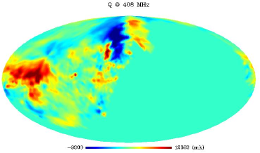
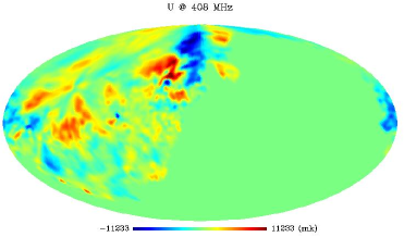
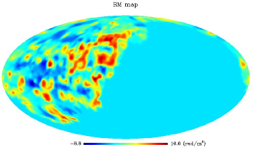
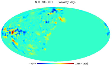
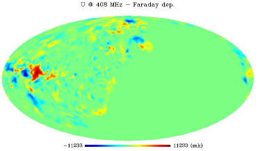
Figure 12: Maps of the Stokes parameters before (upper panels) and after (lower panels) the transformation for Faraday depolarization. In the middle is placed the $RM$ map used in the simulation. All maps have been smoothed to $2.3^{\circ}$. In the depolarized maps the large scale structure appear significantly depressed respect to the input ones, whereas the small scale structures are more relevant.

In Fig. 13 we compare the APSs of the input and the output maps at both the frequencies. At 1420 MHz the APSs are almost identical; on the contrary at 408 MHz the depolarized map APSs significantly flatten, as expected from the increase of small scale features. This supports the interpretation of the bulk of the APS flattening with decreasing frequency resulting from our analysis of the Leiden surveys in terms of the Faraday depolarization effect.

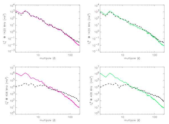
Figure 13: $E$ and $B$ modes APSs before (solid lines) and after (dashed lines) the transformation according to Faraday depolarization. The upper panels refer to 1420 MHz and the lower ones to 408 MHz. The different importance of the depolarization effects at the two frequencies is evident: the 1420 MHz APSs are almost unaffected, whereas the 408 MHz APSs significantly flatten.

8 Discussion and conclusions

The Leiden surveys have been up to now the only available data at $\nu\sim 1$ GHz suitable for a multifrequency study of the polarized diffuse component of the Galactic synchrotron emission on large angular scales. A linear polarization survey of the Southern sky had previously been carried out at 408 MHz using the Parkes telescope (Mathewson & Milne (1965)); unfortunately these data have never been put in digital form. In Fig. 14 an image of the data from this survey has been combined with the Leiden survey at 408 MHz to show an all-sky linear polarization map.

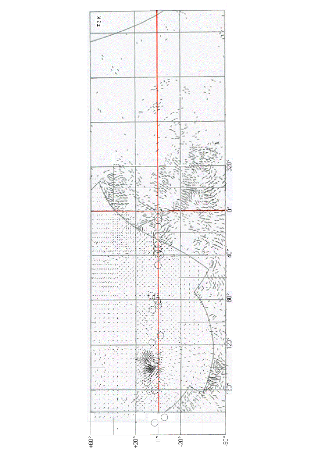
Figure 14: Map of polarization vectors at 408 MHz, obtained combining the corresponding figures of the Leiden survey (Brouw & Spoelstra 1976) and of the Parkes southern sky survey (Mathewson & Milne (1965)). Unfortunately, the vector length has a different scale in the two original figures, therefore only a direct comparison of the direction is feasible.

The “North Polar Spur”, the “Fan Region”, and the “Cetus Arc” (see Berkhuijsen (1971) for a sketch of the Galactic Loops these structures are thought to belong to) are visible as areas where the polarization vectors are longer (the length is proportional to the polarized intensity) and more regularly aligned, drawing small circles in the sky. The most plausible theory suggests that these Galactic spurs are the brighter ridges of evolved Supernova Remnant sitting relatively close to the Sun (within a few $\times 10^{2}$ pc) and obscuring our view of the Galactic diffuse non-thermal emission. The APSs obtained for these regions will be characterized by an amplitude considerably higher than the average, representing therefore an upper limit for the polarized signal of the Galactic synchrotron radiation. On the other hand, the APS should be steeper in these regions, since the polarization vectors appear rather ordered and with approximately constant length, implying a relatively low fluctuation power at small scales. These considerations should be kept in mind when extrapolating the results to the microwave range in order to check the impact of the Galactic synchrotron emission on CMB polarization measurements.
Implementing an interpolation method to deal with the sparse and irregular sampling of the Leiden surveys, we produced maps of $PI$, $Q$ and $U$ with $\theta_{pixel}\simeq 0.92^{\circ}$ at five frequencies between 408 and 1411 MHz. We accomplished several tests in order to check the reliability of the interpolation algorithm and to optimize its quality (see Sects. 3 and 4). We emphasize that the APSs computed from our maps are significantly different from those obtained by other authors (e.g. Bruscoli et al. (2002)) for similar areas of the sky, using the same data; namely, at the higher frequencies of the Leiden surveys we find steeper APSs (first recognized in Burigana & La Porta (2002)). A firm confirmation of our approach comes from the comparison of the APSs obtained for the 1411 MHz map with those of a preliminary version of the DRAO 1420 MHz survey, characterized by much denser sampling and higher sensitivity.

We used the interpolated full coverage maps to study the APS of the polarized synchrotron emission on the multipole range [2,50], being limited at high $\ell$ by the map sensitivity (related to the accuracy and sampling of the original data). Exploiting some better sampled regions, approximately coinciding with the two most prominent Galactic spurs, we could extend our analysis up to $\ell\sim 100$.

At each frequency the APSs of the entire coverage maps turn out to change slope at $\ell\sim 10$, $C_{\ell}^{PI}$, $C_{\ell}^{E}$, and $C_{\ell}^{B}$ presenting a steepening going from the lower to the higher multipoles (see Sect. 5). A general and remarkable result (see Sect. 5) is that the slope of the polarized synchrotron emission APS increases from 408 MHz to 1411 MHz; it changes from $\alpha\sim-(1$-1.5) to $\alpha\sim-(2$-3) for $\ell\sim 10$ to $\sim 100$ and from $\alpha\sim-0.7$ to $\alpha\sim-1.5$ for lower multipoles, the exact value depending on the considered sky region and polarization mode.
One possible explanation for such a behaviour of the APS relies on Faraday depolarization arguments. Fluctuations of the electron density and/or of the magnetic field (in strength and/or direction) might redistribute the synchrotron emission power from the larger to the smaller angular scales, creating fake structures. The effect is more relevant at lower frequencies, where the APS slope is expected to become flatter. We have verified this interpretation by performing a toy-simulation of pure Faraday depolarization in a simple slab model. We note that in the better sampled patches the polarization vectors are well ordered and similarly distributed at 820 MHz and 1411 MHz, which is consistent with the slab model assumptions at least for the considered angular scales. We reproduced the effects of Faraday depolarization on simulated polarized intensity maps, representing the intrinsic Galactic synchrotron emission at 408 MHz and 1420 MHz. We constructed an $RM$ map interpolating the data of Spoelstra (1984) and applied it to transform the input maps according to Faraday depolarization formulae. At 1420 MHz the input and output maps are almost identical, whereas at 408 MHz the large-scale structure of the output map appears depressed and the small scale structures more abundant. Consequently, the corresponding 408 MHz APSs are flatter than the original ones (see Sect. 7.2 for a more precise description of the simulation process). It is therefore preferable to extrapolate the results (spectral index and amplitude of the APS) obtained at 1411 MHz (significantly less affected by Faraday depolarization effect than those at 408 MHz) to estimate the synchrotron APS at microwave frequencies.

By interpreting the ratios of the APS amplitudes at 820 and 1411 MHz (the latter smoothed to the lower angular resolution of the former) in terms of synchrotron emission depolarized by Faraday effect, we have identified possible $RM$ ranges (see Sect. 7.1). This seems a reasonable approach at least in the case of patch 1, 2, and 3, since the polarization vectors are mostly aligned, indicating rather homogeneous physical conditions. Furthermore, taking into account the upper limit to $RM$ derived from the available information on the degree of polarization at 1.4 GHz and considering that the maximum theoretical degree of synchrotron polarization is $\sim 75\%$, we could break or, at least, reduce the degeneracy between the identified $RM$ intervals. For the three better sampled patches, the most reasonable value of $RM$ are $\sim 9-17$ rad/m². However, given the uncertainty on the measured polarization degree, $RM$ values in the interval $\sim 53-59$ rad/m² cannot be excluded. Higher frequencies observations (at $\nu\,\lower 2.0pt\hbox{${>\atop\hbox{\raise 4.0pt\hbox{$\sim$}}}$}\,2$-3 GHz) would be extremely useful to break the degeneracy left by the available $\sim 1$ GHz data.