COSMOGRAIL: the COSmological MOnitoring of GRAvItational Lenses IV.

Abstract

Aims. To predict time delays for a sample of gravitationally lensed quasars and to evaluate the accuracy that can be realistically achieved on the value of $H_{0}$.

Methods. We consider 14 lensed quasars that are candidates for time-delay monitoring and model them in detail using pixelized lens models. For each system, we provide a mass map, arrival-time surface and the distribution of predicted time-delays in a concordance cosmology, assuming $H_{0}^{-1}=14$ Gyr ($H_{0}=70$ in local units). Based on the predicted time-delays and on the observational circumstances, we rate each lens as ‘excellent’ or ‘good’ or ‘unpromising’ for time-delay monitoring. Finally, we analyze simulated time delays for the 11 lens rated excellent or good, and show that $H_{0}$ can be recovered to a precision of 5%.

Results. In combination with COSMOGRAIL paper I on the temporal sampling of lensed quasar light curves, the present work will help design monitoring campaigns of lensed quasars.

1 Introduction

Gravitational lensing of distant quasars is one of many possible routes to $H_{0}$. It has unique advantages. First, lensing depends on well-understood physics: gravitation. Second, time-delay observations require modest resources, hence low-demand telescopes can make a significant contribution. Third, the galaxy models used to convert time-delays into $H_{0}$ have made considerable progress in the past decade. As a result, time-delay measurements have become an increasingly active research topic. So far there are 12 secure time-delays (Table 1), of which 10 yield an estimate of the Hubble constant — the lens identification in PKS 1830–211 remains controversial (Courbin et al. (2002), Winn et al. (2002)), and the lensing galaxy HE 0435–122 may be anomalous (Kochanek 2005).

The dominant uncertainty in measuring $H_{0}$ from lensing is the non-uniqueness of lens mass profiles that can reproduce the observables. Before the non-uniqueness of mass-models was widely appreciated, researchers would usually fit a single family of mass models to data, leading to over-optimistic error bars. Experimenting with different kinds of mass model for the same data pointed to much larger uncertainties (Schechter et al. 1997, Saha & Williams (1997); Bernstein & Fischer (1999); Keeton et al. (2000)). More recently, procedures involving sampling an ensemble of models according to some prior are being preferred, in order to derive a more useful picture of the uncertainties (Williams & Saha (2000); Saha & Williams (2004); Oguri et al. 2004a , Jakobsson et al. 2005). A fair summary of current $H_{0}$ results from lensing is that the error-bars are competitive on the young-Universe (i.e., high $H_{0}$) side but the old-Universe side needs improvement.

Clearly, to reach the 5–10% accuracy claimed by some other techniques (e.g., Freedman et al. (2001); Spergel et al. (2003)), more time-delays are needed. But to run monitoring campaigns efficiently, it is important to have preliminary estimates for time-delays — witness the tenfold range in the known values in Table 1 — as well as to identify the most promising systems to monitor. This paper supplies such information. For a sample of 14 lenses we provide predicted time delays with uncertainties, a rating of prospects as ‘excellent’, ‘good’, or ‘unpromising’ based on both models and the observational situation, and finally an estimate of the precision on $H_{0}$ obtainable from these lenses. A companion paper by Eigenbrod et al. (2005; COSMOGRAIL I) is devoted to the determination of the optimal strategy to use in order to measure time-delays (temporal sampling of the light curves, object visibility and variability, contamination by microlensing, etc). Together, these papers help design an observational campaign.

An ideal time-delay lensing system has the following features: 1- bright optical images, 2- large angular image separations ($>$1″), 3- light path unperturbed by nearby structure, 4- known or easy-to-measure lens redshift $z_{\rm lens}$. Our sample of 14 has been selected using these criteria as a guideline, though not a strict requirement. We have considered only objects for which the time-delay can be measured in the optical.

The main results of this paper are in Sect. 3 and 4, which present ensembles of models for the 14 individual systems and then estimate the precision to which $H_{0}$ could be recovered from them. But before going into details of the models, it is useful to preview the results and compare them with measured systems. We do this in Sect. 2.

2 Comparing observed and predicted delays

It is possible to make a preliminary prediction of time delays from image positions before any modelling, by recalling the scales involved.

In lensing theory, the geometric part of the time delay is of the order of the image-separation squared times $DH_{0}^{-1}$, where $D$ is the usual dimensionless distance factor depending on cosmology. The total time delay will be smaller but of the same order. Saha (2004) shows that the longest time delay can be expressed as

$$\Delta t=\varphi D\left[{\textstyle\frac{1}{16}}(\theta_{1}+\theta_{2})^{2}\,H_{0}^{-1}\right]$$ (1)

where where $\theta_{1},\theta_{2}$ are the lens-centric distances (in radians) of the first and last images to arrive and $\varphi$ is a dimensionless factor that ranges within about 0–2 for quadruples and 2–6 for doubles. The expression in square brackets in Eq. (1) has the elegant interpretation of the fraction of the sky covered by the lens, times $H_{0}^{-1}$.

We now define an ‘astrometric time delay’ $\Delta t_{\rm astrom}$ by taking Eq. (1) and setting $\varphi$ to a fiducial value of 1.5 for all quadruples and 4 for all doubles. This is a useful preliminary predictor of time delays, as we will see below.

Table 1: The 12 time-delays measured so far, with 1$\sigma$ error bars. Lens redshifts in parenthesis are either photometric or based on absorption lines in the quasar images.

$$\begin{array}[]{p{2cm}p{1cm}cccl}\hline\cr\vskip 3.0pt plus 1.0pt minus 1.0pt\cr Object&Type&z_{\rm lens}&\Delta t_{\rm astrom}&&\Delta t_{\rm obs}\\ \vskip 3.0pt plus 1.0pt minus 1.0pt\cr\hline\cr\vskip 3.0pt plus 1.0pt minus 1.0pt\cr B0218+357&AD&0.68&10&&\phantom{0}10\pm 1^{\mathrm{a},b}\\ J0951+263&ID&(0.24)&11&&\phantom{0}16\pm 2^{\mathrm{c}}\\ B1115+080&IQ&0.31&24&&\phantom{0}25\pm 4^{\mathrm{d},e}\\ B1600+434&AD&0.41&35&&\phantom{0}51\pm 4^{\mathrm{f}}\\ B0435--122&CQ&0.46&41&&\phantom{0}14\pm 1^{\mathrm{g}}\\ B1830--211&AD&(0.89)&42&&\phantom{0}26_{-4}^{+5}{}^{\mathrm{h}}\\ B2149--274&AD&0.50&59&&103\pm 12^{\mathrm{i}}\\ B1608+656&IQ&0.63&60&&\phantom{0}77\pm 3^{\mathrm{j}}\\ B1520+530&ID&0.72&92&&130\pm 3^{\mathrm{k}}\\ J0911+055&SQ&0.77&119&&146\pm 8^{\mathrm{l}}\\ B1104--181&AD&0.73&345&&161\pm 7^{\mathrm{m}}\\ B0957+561&ID&0.36&536&&423\pm 1^{\mathrm{n}}\\ \vskip 3.0pt plus 1.0pt minus 1.0pt\cr\hline\cr\end{array}$$

^aCohen et al. (2000)      ^bBiggs et al. (1999)  ^cJakobsson et al. (2005)  ^dSchechter et al. (1997)  ^eBarkana (1997)           ^fBurud et al. (2000)  ^gKochanek et al. (2005)  ^hLovell et al. (1998)  ⁱBurud et al. (2002a)  ^jFassnacht et al. (2002)  ^kBurud et al. (2002b)  ^lHjorth et al. (2002)  ^mOfek & Maoz, D. (2003)  ⁿOscoz et al. (2001)

Figure 1: Plot of $\Delta t_{\rm obs}$ against $\Delta t_{\rm astrom}$ for the known time-delay systems, showing that known and prospective systems can be easily compared. Squares denote quadruple systems, triangles are for doubles.

Table 2: Predicted time-delays (and 1$\sigma$ error bars) sorted by increasing astrometric delay, for objects with no measured time-delay. Lens redshifts in parenthesis are either photometric or based on absorption lines in the quasar images.

$$\begin{array}[]{p{2cm}p{1cm}cccl}\hline\cr\vskip 3.0pt plus 1.0pt minus 1.0pt\cr Object&Type&z_{\rm lens}&\Delta t_{\rm astrom}&&\Delta t_{\rm pred}\\ \vskip 3.0pt plus 1.0pt minus 1.0pt\cr\hline\cr\vskip 3.0pt plus 1.0pt minus 1.0pt\cr B1422+231&LQ&0.34&8&&18_{-5}^{+5}\\ J2026--453&IQ&(0.5)&14&&15_{-6}^{+2}\\ J1155+634&AD&0.18&19&&35_{-10}^{+8}\\ J0924+021&IQ&0.39&19&&12_{-4}^{+6}\\ J1650+425&ID&(0.5)&46&&54_{-13}^{+8}\\ J1335+011&AD&0.44&47&&49_{-16}^{+13}\\ J1355--225&AD&(0.70)&68&&89_{-39}^{+28}\\ J1131--123&LQ&0.30&69&&137_{-39}^{61}\\ J2033--472&IQ&0.66&70&&72_{-20}^{+33}\\ B1030+074&AD&0.60&75&&153_{-57}^{+29}\\ B0909+532&ID&(0.83)&90&&72_{-17}^{+10}\\ B1009--025&AD&0.87&98&&161_{-59}^{+34}\\ B0818+122&ID&0.39&111&&110_{-26}^{+16}\\ J0903+502&ID&0.39&122&&110_{-23}^{+13}\\ \vskip 3.0pt plus 1.0pt minus 1.0pt\cr\hline\cr\end{array}$$

Figure 2: Plot of $\Delta t_{\rm pred}$ against $\Delta t_{\rm astrom}$ for the prospective time-delay systems. Error bars are 68% confidence. Squares denote quadruple systems, triangles are for doubles.

Figure 3: Plot of $\Delta t_{\rm pred}$ against $\Delta t_{\rm obs}$ for the current time-delay systems. Again, squares are for quadruple systems, triangles for doubles.

Table 1 gives the astrometric and actual observed time delays for the 11 known time-delay systems (disregarding here the middle two images in quadruples, i.e., images 2 and 3 in the figures). The ‘type’ refers to the morphological classification introduced in Saha & Williams (2003): $\hbox{AD}=\hbox{axial}\ \hbox{double,}$ $\hbox{ID}=\hbox{inclined}\ \hbox{double,}$ $\hbox{CQ}=\hbox{core}\ \hbox{quad,}$ $\hbox{LQ}=\hbox{long-axis}\ \hbox{quad,}$ $\hbox{SQ}=\hbox{short-axis}\ \hbox{quad,}$ $\hbox{IQ}=\hbox{inclined}\ \hbox{quad.}$

Fig. 1 plots the data summarized in Table 1. It is striking that while $\Delta t_{\rm obs}$ ranges over a factor of 40, it tracks $\Delta t_{\rm astrom}$ to a factor of 2.

Fig. 2 and Table 2 summarize our time-delay predictions. To make these predictions we used the PixeLens code (Saha & Williams (2004)) to generate an ensemble of 200 models for each lens, leading to an ensemble of model time-delays, which we interpret as the probability distribution for the predicted time-delays.

How reliable are the time-delay predictions? Pixellated models generically involve a choice of prior (also called secondary constraints); if the prior is too different from what lenses are really like then the results will be incorrect. Our prior is basically the PixeLens default; in detail, we assumed the following:

1. In most cases we required the mass profile to be inversion-symmetric about the lens centre. But if the lensing galaxy appeared very asymmetric, or the image morphology was unusual, we let the mass profile be asymmetric.

2. If there was evidence of external shear from the lens environment and/or the image morphology, we allowed the code to fit for constant external shear. That is to say, we allowed a contribution of the form $\gamma_{1}(\theta_{x}^{2}-\theta_{y}^{2})+2\gamma_{2}\theta_{x}\theta_{y}$ to the arrival time, with adjustable constants $\gamma_{1},\gamma_{2}$.

3. The density gradient must point within $45^{\circ}$ of the lens center (thus ensuring that the lens is centrally concentrated).

4. The radial mass profile must be steeper than $\theta^{-0.5}$. That implies a 3D profile steeper than $r^{-1.5}$, which is consistent with available estimates from stellar or gas dynamics; for example, Binney et al. (1991) report an $r^{-1.75}$ profile near the Galactic centre.

5. The density on any pixel must be $\leq$ twice the average of its neighbours, except for the central pixel, which can be arbitrarily dense.

As a test we ‘postdicted’ the time-delays in the known systems. The results are summarized in Fig. 3. We find that our prior tends to overestimate the time-delays for the systems with the largest angular separations, perhaps because these lenses have a significant cluster contribution and the profiles are much shallower than in our prior. One of the discrepant lenses is PKS 1830-211, which has a double lens galaxy. The two others are B0957$+$561 and J0911$+$055, which both have significant contribution by a group or cluster of galaxies along the line of sight. But predicted time delays of less than 200 days appear reliable. The candidate lenses are all in the reliable regime.

3 Individual systems

We now proceed to discuss individual lenses, grouped by similar morphology.

For each lens, we show three kinds of plot. First, there is a mass map of the ensemble-average model. The contours in the mass maps are in logarithmic steps, with each step corresponding to a factor of $10^{0.4}$ (like a magnitude scale). The critical density contour is always the third from outermost. Second, we have plots showing saddle-point contours. These plots also show the source position in the ensemble-average model. The detailed placement of the saddle-point contours and the inferred source varies across the ensemble, but the qualitative features are robust. In particular, the saddle-point contours make the time-ordering of images obvious. We will refer to individual images by their time order: 1,2 for doubles or 1,2,3,4 for quadruples, meaning that the image labelled 1 varies first, then 2, etc. Third, we have histograms for the predicted time delays between different pairs of images in each lens.

After modelling each lens, we rate its prospects as a time-delay system as ‘excellent’, ‘good’, or ‘unpromising’, based on how well-constrained the time-delays are and on the comparative ease of monitoring and photometry.

We remark that the modelling process really produces a predicted distribution for $H_{0}\,\Delta t$. In the present work we insert a fiducial value of $H_{0}$ to obtain a distribution for $\Delta t$, but one can equally insert a measured value of $\Delta t$ (if available) and obtain a distribution for $H_{0}$. But if two or more time delays become available for a quadruple, their ratio provides a new constraint on the lens, and the modelling code must be run again.

3.1 Axial doubles

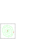
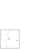
Figure 4: Models of J1155+634 (axial double). See text in section 3 for the format. Prospects: unpromising.

J1155+634 [Fig. 4] discovery: Pindor et al. (2004). The separation $\Delta\theta=1.83^{\prime\prime}$ is relatively large, but the lens galaxy is only $\sim 0.2^{\prime\prime}$ from the fainter image. Also, the measurement $z_{\rm lens}=0.1756$ is somewhat insecure because the inferred galaxy absorption features are amongst the Ly$\alpha$ forest lines. As a time-delay prospect, this system appears unpromising.

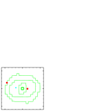
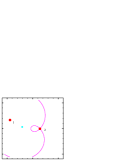
Figure 5: Models of J1355–225 (axial double). Prospects: good.

J1355–225 [Fig. 5] discovery: Morgan et al. (2003a); also known as CTQ 327. The quasar images are bright and the angular separation is moderate: $\Delta\theta=1.22^{\prime\prime}$. Models include external shear corresponding to further mass to the NW or SE. We rate this system as a good time-delay prospect.

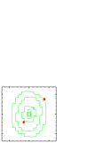
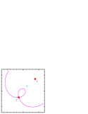
Figure 6: Models of J1335+011 (axial double). Prospects: excellent.

J1335+011 [Fig. 6] discovery: Oguri et al. (2004b). We rate this system as an excellent time-delay prospect.

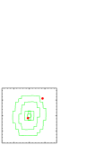
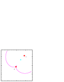
Figure 7: Models of B1030+074 (axial double). Prospects: unpromising.

B1030+074 [Fig. 7] discovery: Xanthopoulos et al. (1998). Like J1155+634 it has a relatively wide separation but a second image is faint and very close to the galaxy. There is evidence for variability. The peak in the predicted time delays near 180 days is interesting, but it is probably not wise to over-interpret, given the resolution of the models used in this paper. Because of the difficulty of accurate photometry on the second image, we rate this system as unpromising.

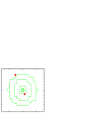
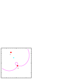
Figure 8: Models of B1009–025 (axial double). Prospects: good.

B1009–025 [Fig. 8] discovery: Surdej et al. (1993). Its clean morphology, evidence of variability and a nearby foreground QSO usable as a standard PSF all make this an attractive target. However, the combination of an approximately half-year time-delay and a near-equatorial location is awkward (see Eigenbrod et al. 2005 for more details). We rate time-delay prospects as good.

3.2 Inclined doubles

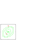
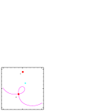
Figure 9: Models of J1650+425 (inclined double). Prospects: excellent.

J1650+425 [Fig. 9] discovery: Morgan et al. (2003b). It has significant external shear, probably from a group galaxy to the E. The high declination of the objects makes it possible to observe it almost continuously from the northern hemisphere. This system is an excellent time-delay prospect.

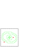
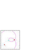
Figure 10: Models of B0909+532 (inclined double). Prospects: excellent

B0909+532 [Fig. 10] discovery as multiply imaged: Kochanek et al. (1997). The lensing galaxy is very faint, which caused some early controversy until the issue was settled by Oscoz et al. (1997) and Lubin et al. (2000). The morphology and models indicate significant external shear from mass to the NE or SW, but the galaxies responsible have not yet been identified. Both quasar images are very bright, and their separation is $\Delta\theta=1.17^{\prime\prime}$. Its $z_{\rm lens}$ is still insecure, but assuming that problem is solved, this system is an excellent prospect.

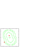
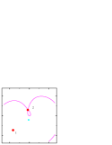
Figure 11: Models of B0818+122 (inclined double). Prospects: good

B0818+122 [Fig. 11] discovery: Hagen & Reimers (2000). A chain of galaxies to the NE contribute a large external shear. The fainter image is very close to the main lensing galaxy, and about the same brightness. Overall, prospects appear good.

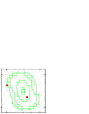
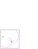
Figure 12: Models of J0903+502 (inclined double). Prospects: good.

J0903+502 [Fig. 12] discovery: Johnston et al. (2003). There are several group galaxies in addition to the main lensing galaxy, with one galaxy to the SW probably the major contributor of external shear. Both quasar images are faint, $R\sim 19-20$, so monitoring is difficult with a 1 m-class telescope. The distribution of predicted time-delays is narrow. Overall, we rate prospects as good.

3.3 Long-axis quadruples

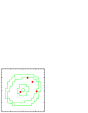
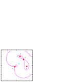
Figure 13: Models of B1422+231 (long-axis quadruple). Prospects: good.

B1422+231 [Fig. 13] discovery: Patnaik et al. (1992). It is a radio emitter with extremely accurate image positions. There is evidence of variability. Strong external shear comes from a galaxy group to the SE. Time-delays between the close triplet of images may be too short to measure in the optical, but the delay to the fourth image can be expected to be useful. The lensing galaxy is comparable in brightness to the faint fourth image, which complicates the photometry. Overall, prospects appear good.

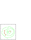
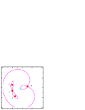
Figure 14: Models of J1131–123 (long-axis quadruple). Prospects: excellent.

J1131–123 [Fig. 14] discovery: Sluse et al. (2003). It is a quadruple with large separation: $3.69^{\prime\prime}$. It is very like a larger sibling of B1422+231. Morphology and models indicate significant external shear from mass to the WNW or ESE. There is evidence for intrinsic variability. Structures in the Einstein ring are likely to offer additional model constraints, though they also contaminate the flux from the faint fourth image. Overall, prospects appear excellent.

3.4 Inclined quadruples

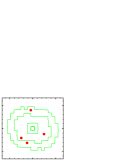
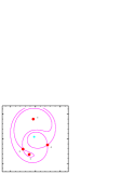
Figure 15: Models of J2026–453 (inclined quadruple). Prospects: good.

J2026–453 [Fig. 15] and J2033–472 [Fig. 16] discovery: Morgan et al. (2004). In J2026-453, morphology and models indicate external shear from mass to the E or W. This system so far lacks a $z_{\rm lens}$; we assumed 0.5, which is plausible given the colours of the galaxy. The morphology of J2033–472 suggests an asymmetric lens, and accordingly we have considered asymmetric models. We rate time-delays prospects as good for J2026 and excellent for J2033.

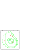
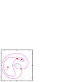
Figure 16: Models of J2033–472 (inclined quadruple). Prospects: excellent.

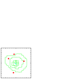
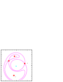
Figure 17: Models of J0924+021 (inclined quadruple). Prospects: currently unpromising.

J0924+021 [Fig. 17] discovery: Inada et al. (2003). This is a complex and evidently asymmetric lens, but can be well-modelled and leads to relatively tight predictions for two of the time delays. However, image 3 is very faint, which Keeton et al. (2005) argue is the result of microlensing. This greatly complicates the measurements of time delays, so we current rate this lens as an unpromising time-delay prospect.

4 Predicted precision for the Hubble time

In the previous section, after considering detailed models as well as observational circumstances of all 15 lenses, we concluded that 5 systems are excellent candidates for time-delay monitoring (J1650+425, J2033–472, B0909+532, J1335+011, J1131–123), and 6 are good candidates (J1355–225, J0903+502, B0818+122, B1009–025, B1422+231, J2026–453). We now ask how accurately $H_{0}^{-1}$ can be inferred if the 5 excellent candidates, or if the 11 excellent or good candidates, have their time delays measured accurate to 1 d. We do not expect that either scenario will be what transpires in the future. We expect that some of these 11 lenses will yield accurate time delays over the next 2–3 years, while some existing time-delay measurements are refined. But the 5-lens and 11-lens cases are reasonable surrogates for a future set of available measurements.

Fig. 18 shows the recovered $H_{0}^{-1}$ from simulated time delays of the 5 excellent candidates. For each lens we took a random model (from the ensemble of 200), read off its time delays rounded to the nearest day, and then took them as simulated time delays. Any model delays of $\leq 1$d we treated as unmeasured. Using PixeLens, we then modelled the 5 lenses simultaneously from the actual image positions and these simulated time delays. The model-ensemble had 200 members, each member consisting of models for all 5 lenses sharing a common $H_{0}^{-1}$ (Saha & Williams (2004)). Fig. 18 shows the resulting 200 values of $H_{0}^{-1}$ after binning. We see that the original input value 14 Gyr is recovered with $<10\%$ uncertainty at 68% confidence, and no discernable bias. Also, the uncertainties are asymmetric.

Fig. 19 shows the result of a similar exercise using the 6 good candidates. The uncertainties are somewhat larger than in Fig. 18 and similarly asymmetric. Also, there is a bias, in the sense that the median value is $15.0$ Gyr rather than $14.0$ Gyr; but the bias is in the 68% confidence range and hence not significant.

The 5-lens and 6-lens ensembles just described are independent. Hence we can simply multiply their histograms. Fig. 20 shows the result. We recover $H_{0}^{-1}$ with an uncertainty of about 5%, at 68% confidence.

Figure 18: Hubble constant/time recovered from simulated time delays of the 5 excellent candidates. The confidence intervals (read off by sorting the unbinned values) are $14.0^{+1.2}_{-0.7}$Gyr at 68% and $14.0^{+2.9}_{-1.3}$Gyr at 90%.

Figure 19: Hubble constant/time from simulated time delays of the 6 good candidates. The confidence intervals are $15.0^{+1.3}_{-1.0}$ Gyr at 68% and $15.0^{+3.7}_{-1.5}$ Gyr at 90%.

Figure 20: Hubble constant/time from simulated time delays of the 11 excellent or good lenses. This histogram is simply the product of the two previous ones. From a narrower binning, we read off the confidence intervals $14.2^{+0.7}_{-0.7}$Gyr at 68% and $14.4^{+1.9}_{-0.8}$Gyr at 90%.

These results show that the Hubble time can be recovered to 5% precision even if we allow for a large diversity in possible mass distributions (or prior). But there is a caveat, which needs to be addressed before a claim of 5% accuracy (rather than precision) can be made. Currently, a mass distribution that satisfies the lensing constraints is either allowed by the prior as a plausible galaxy lens, or rejected; there is no weighting in the prior. Properly, the prior should weight mass models according to their abundance in the real world of galaxies. Lack of weighting will introduce a bias. (This prior-induced bias is different from the small statistical bias seen in Fig. 19.) The blind tests in Williams & Saha (2000) would have detected biases if they were around 20% or more. But prior-induced biases at the 5% level remain untested for. Finding them and then eliminating them through a weighted prior could be done by calibrating against galaxy-formation models, and is an essential theoretical program needed to complement the observations.

5 Discussion

In this paper we do three things: first, we introduce a simple rough predictor for time delays $\Delta t_{\rm astrom}$, second, we make model predictions for 23 time delays covering 14 lenses, and finally we estimate the precision in the Hubble time inferred from simulated data on the 11 best lenses. The main conclusion is that no single lens can usefully constrain $H_{0}$, but time delays accurate to $\simeq 1$d on $>10$ lenses can yield $H_{0}$ accurate to 5%.

In the histograms in Figs. 4–17, typically 90% of the area ranges over a factor of two in time delays. Hence, a monitoring program can have 90% confidence in succeeding — provided the quasar is sufficiently variable — if the sampling allows for the appropriate 90%-range of possible time delays. There is no single characteristic shape for the histograms, but the pattern of a low-end tail and a high-end cliff is common. The large uncertainty in the predicted time delays reflects the large variety of mass models models that can reproduce the observed image positions in any given lens. The prior we have for deciding what is an allowable mass model for a galaxy is very conservative, so our models have more variety than reality. But not very much more — if all real galaxy lenses belonged to some known parametrization, then error-bars on $H_{0}$ from fitting such parametric models to observed time-delay systems would overlap, but as is evident from Fig. 12 in Courbin (2003), those error-bars do not overlap.

Actually, the basic results about predicted time delays are already present in the summaries Figs. 1 and 2. To interpret these figures, recall that $\Delta t_{\rm astrom}$ makes a preliminary prediction for the time-delay, while the deviation from the oblique line depends on the details of mass distribution and lens morphology. From Fig. 1 we see that $\Delta t_{\rm astrom}$ gets us to within a factor of two of the observed values. Now, the error bars —note that the error bars in tables and figures are 68% confidence— in Fig. 2 are generally less than a factor of two; thus detailed modelling does provide a better prediction than $\Delta t_{\rm astrom}$ alone, but not dramatically better. We can also see that several of the error bars in Fig. 2 are shorter on top, thus indicating a low-end tail and a high-end cliff.

The image morphology of a lens is correlated with the uncertainty in the time delays, especially in quadruples. Core quadruples generically have short time delays and are unlikely to be useful for time delays; the case of B0435-122 is illustrative. Long- and short-axis quadruples, having three images close together, are likely to have only one measurable time delay. Inclined quadruples are the most promising, since they usually have two time delays in the measurable range, and sometimes three. Among doubles, inclined systems tend to be somewhat better constrained than axial systems. Significant asymmetry in the lens is a disadvantage, but in compensation, asymmetry increases the chance of having three measurable time delays. Thus B1608+656 is an asymmetric inclined quadruple with three measured time delays; J2033–472 may prove to be another, and is among our excellent candidates. Surprisingly, a large external shear appears to reduce uncertainties in the time delay. This is particularly noticeable in the inclineddoubles J1650+425, B0909+532, and J0903+502, and the short-axis quads B1422+231 and J1131–123. The reason is not clear; it may be that since external shear reduces amount of mass needed in the main lens to produce multiple images, it reduces the available model-space.

Finally, the results from combining several lenses are very encouraging. Assuming time delays accurate to 1 d we find that the model-dependent uncertainty in $H_{0}^{-1}$ reduces to less than 10% on combining the 5 best lenses, and about 5% on combining the best 11 lenses. The uncertainties are asymmetric, with the lower limit on the Hubble time being tighter than the upper limit. More work needs to be done on the model prior before we can truly attain 5% accuracy, but meanwhile our results help provide both motivation and observing strategies for accurate time-delay measurements.