Percolation Galaxy Groups and Clusters in the SDSS Redshift Survey: Identification, Catalogs, and the Multiplicity Function

Abstract

We identify galaxy groups and clusters in volume-limited samples of the SDSS redshift survey, using a redshift-space friends-of-friends algorithm. We optimize the friends-of-friends linking lengths to recover galaxy systems that occupy the same dark matter halos, using a set of mock catalogs created by populating halos of N-body simulations with galaxies. Extensive tests with these mock catalogs show that no combination of perpendicular and line-of-sight linking lengths is able to yield groups and clusters that simultaneously recover the true halo multiplicity function, projected size distribution, and velocity dispersion. We adopt a linking length combination that yields, for galaxy groups with ten or more members: a group multiplicity function that is unbiased with respect to the true halo multiplicity function; an unbiased median relation between the multiplicities of groups and their associated halos; a spurious group fraction of less than $\sim 1\%$; a halo completeness of more than $\sim 97\%$; the correct projected size distribution as a function of multiplicity; and a velocity dispersion distribution that is $\sim 20\%$ too low at all multiplicities. These results hold over a range of mock catalogs that use different input recipes of populating halos with galaxies. We apply our group-finding algorithm to the SDSS data and obtain three group and cluster catalogs for three volume-limited samples that cover 3495.1 square degrees on the sky, go out to redshifts of 0.1, 0.068, and 0.045, and contain 57138, 37820, and 18895 galaxies, respectively. We correct for incompleteness caused by fiber collisions and survey edges, and obtain measurements of the group multiplicity function, with errors calculated from realistic mock catalogs. These multiplicity function measurements provide a key constraint on the relation between galaxy populations and dark matter halos.

1. Introduction

Galaxies are gregarious by nature. Bright galaxies typically reside in groups or clusters, surrounded by less luminous neighbors. Interactions within the group or cluster environment may have important effects on the star formation history, morphology, dynamics, and other properties of member galaxies. Characterizing the relation between galaxy properties and their group environment is thus a key step in understanding galaxy formation and evolution. At the density thresholds often used to identify groups, most members should belong to the same, gravitationally bound dark matter (DM) halo. Recent approaches to describing the relation between galaxies and DM focus on galaxy populations of DM halos as a function of halo mass. Specifically, the bias of a particular class of galaxies can be characterized by its Halo Occupation Distribution (HOD), which specifies the probability distribution $P(N|M)$ that a halo of mass $M$ contains $N$ such galaxies, together with relations describing the relative spatial and velocity distributions of galaxies and dark matter within halos (berlind_weinberg_02 and references therein). A well defined group catalog with well understood properties can play a central role in the empirical determination of this relation.

This paper presents a group and cluster catalog defined from the Sloan Digital Sky Survey (SDSS, york_etal_00). While this catalog is useful for many purposes, our overriding objective is to obtain a well understood measurement of the group multiplicity function (the space density of groups as a function of richness), with the goal of determining the HOD in the high mass regime (peacock_smith_00; berlind_weinberg_02; marinoni_hudson_02; kochanek_etal_03; lin_etal_04). With this objective in mind, we have adopted a simple group-finding algorithm, friends-of-friends in redshift space (huchra_geller_82), and carried out extensive tests on realistic mock catalogs in order to assess its performance and optimize parameter choices. We apply the group-finding algorithm to volume-limited samples of galaxies so that the resulting group statistics characterize the clustering of well defined populations of galaxies.

Galaxy clusters have been the focus of study since they were first seen on optical photographic plates (shapley_ames_26). zwicky_37 pioneered the study of clusters as dynamical objects by using imaging and spectroscopy of the Coma cluster to estimate its mass. However, the most influential pioneering work on clusters was done by abell_58, who assembled the first large sample of galaxy clusters. The Abell catalog of rich galaxy clusters (abell_58; abell_etal_89) was created by eyeball identification in the Palomar Observatory Sky Survey and it spawned numerous follow-up studies. devaucouleurs_71 shifted focus to poorer systems by studying nearby groups of galaxies. gott_turner_77b made the first measurement of the group multiplicity function using the (turner_gott_76) catalog of groups selected based on the projected surface density of galaxies.

With the advent of large redshift surveys, group identification became three dimensional and thus less subject to projection effects. Group-finding in redshift space was pioneered by huchra_geller_82 and geller_huchra_83, using the Center for Astrophysics (CfA) redshift survey. Subsequent versions of the CfA redshift survey were used to identify groups by various authors (nolthenius_white_87; ramella_etal_89; moore_etal_93; ramella_etal_97). Other redshift surveys that spawned group catalogs were the Nearby Galaxies Catalog (tully_87), the ESO Slice Project (ramella_etal_99), the Las Campanas Redshift Survey (LCRS) (tucker_etal_00), the Nearby Optical Galaxy Sample (NOG) (giuricin_etal_00), the Southern Sky Redshift Survey (SSRS) (ramella_etal_02), the 2dF redshift survey (merchan_zandivarez_02; eke_etal_04a; yang_etal_05), and even the high redshift DEEP2 survey (gerke_etal_05).

There have been several efforts to detect clusters in the SDSS to date, most of them using the photometric data rather than the redshift data. annis_etal_99 developed the maxBCG technique, where Brightest Cluster Galaxy (BCG) candidates are identified based on their colors and magnitudes and other cluster members are selected from nearby galaxies that have the colors of the E/S0 ridgeline. kim_etal_02 developed a hybrid matched filter (HMF) technique that assumes a radial profile for clusters and convolves the data with that filter. goto_etal_02 developed the cut-and-enhance (CE) method, which selects overdensities of galaxies that have similar colors. All these techniques were applied to the early SDSS commissioning data (bahcall_etal_03; goto_etal_02). lee_etal_04 identified compact groups by looking for small and isolated concentrations of galaxies in the SDSS Early Data Release (EDR; stoughton_etal_02). Cluster searches in the SDSS redshift survey have also been carried out. goto_etal_05 used a friends-of-friends algorithm (though with linking lengths that do not scale with the changing number density of galaxies due to the flux limit) to identify clusters in the SDSS Data Release 2 (DR2; abazajian_etal_04). merchan_zandivarez_05 used a friends-of-friends algorithm to identify groups in the SDSS Data Release 3 (DR3; abazajian_etal_05). weinmann_etal_05 used the yang_etal_05 algorithm to identify groups in SDSS DR2. miller_etal_05 developed the C4 algorithm for finding clusters in redshift space and also applied it to the SDSS DR2. The C4 algorithm looks for concentrations of galaxies in a seven-dimensional position and color space. It takes advantage of the color similarity of cluster member galaxies and thus minimizes contamination due to projection. However, some correlations are built into the method, and modeling it in order to understand the properties of the resulting cluster catalog requires a complete model of the galaxy population (including colors and luminosities). Our method complements the C4 catalog by applying a simple and easily modeled algorithm to volume-limited samples with homogeneous properties.

In § 2 we describe the SDSS data that we use. In § 3 we describe the mock catalogs that we use to optimize our group-finder and to estimate uncertainties for our measured group statistics. In § 4 we outline our group-finding algorithm and choice of parameters. We present a detailed discussion of tests with mock catalogs in the Appendix, with the key points summarized in the main text. We discuss incompleteness in our group catalogs due to fiber collisions and survey edges in § 5. The group catalogs are published in electronic tables and their contents are described in § 6. Finally, in § 7, we present our measured group multiplicity function. We will use this to constrain the HOD in future work. We summarize our results in § 8.

2. Data

2.1. SDSS

The SDSS is a large imaging and spectroscopic survey that is mapping two-fifths of the Northern Galactic sky and a smaller area of the Southern Galactic sky, using a dedicated 2.5 meter telescope (gunn_etal_06) at Apache Point, New Mexico. The survey uses a photometric camera (gunn_etal_98) to scan the sky simultaneously in five photometric bandpasses (fukugita_etal_96; smith_etal_02) down to a limiting $r$-band magnitude of $\sim 22.5$. The imaging data are processed by automatic software that does astrometry (pier_etal_03), source identification, deblending and photometry (lupton_etal_01; lupton_05), photometric calibration (hogg_etal_01; smith_etal_02; tucker_etal_05), and data quality assessment (ivezic_etal_04). Algorithms are applied to select spectroscopic targets for the main galaxy sample (strauss_etal_02), the luminous red galaxy sample (eisenstein_etal_01), and the quasar sample (richards_etal_02). The main galaxy sample is approximately complete down to an apparent $r$-band Petrosian magnitude limit of $<17.77$. Targets are assigned to spectroscopic plates using an adaptive tiling algorithm (blanton_etal_03a). Finally, spectroscopic data reduction pipelines produce galaxy spectra and redshifts.

We use the large-scale structure sample sample14 from the NYU Value Added Galaxy Catalog (NYU-VAGC; blanton_etal_04a) as our primary galaxy sample. Galaxy magnitudes are corrected for Galactic extinction (schlegel_etal_98) and absolute magnitudes are k-corrected (blanton_etal_03b) and corrected for passive evolution (blanton_etal_03c) to rest-frame magnitudes at redshift $z=0.1$. A significant fraction of the sample that we use was made publicly available with the SDSS Data Release 3 (abazajian_etal_05).

Table 1. Volume-limited Sample Parameters

Name	$z_{\mathrm{min}}$	$z_{\mathrm{max}}$	$<M_{{}^{0.1}\!{r}}$	$N_{\mathrm{g}}$	$\bar{n}_{\mathrm{g}}$
$Mr20$	0.015	0.100	-19.9	57138	0.00673
$Mr19$	0.015	0.068	-19.0	37820	0.01396
$Mr18$	0.015	0.045	-18.0	18895	0.02434

Note—Absolute magnitude thresholds listed are for $z_{\mathrm{max}}$. $\bar{n}_{\mathrm{g}}$ is in units of $h^{3}{\mathrm{Mpc}}^{-3}$.

The galaxy redshift sample has an incompleteness due to the mechanical restriction that spectroscopic fibers cannot be placed closer to each other than their own thickness. This fiber collision constraint makes it impossible to obtain redshifts for both galaxies in pairs that are closer than $55^{\prime\prime}$ on the sky. In the case of a conflict, the target selection algorithm randomly chooses which galaxy gets a fiber (strauss_etal_02). Spectroscopic plate overlaps alleviate this problem to some extent, but fiber collisions still account for a $\sim 6\%$ incompleteness in the main galaxy sample. Since this incompleteness is most severe in regions of high galaxy density, it is necessary to correct for it in studies of groups and clusters. We correct for fiber collisions by giving each collided galaxy the redshift of its nearest neighbor on the sky (usually the galaxy it collided with), and we show in § 5 that this procedure is adequate for our purposes. Putting collided galaxies at the redshifts of their nearest neighbors will cause some nearby galaxies to be placed at high redshift, artificially making their estimated luminosities very high. Since the abundance of highly luminous galaxies is low, this contamination can become a significant fraction of all highly luminous galaxies. For this reason, we also give collided galaxies the magnitudes (in addition to the redshifts) of their nearest neighbors. The resulting luminosity distribution is thus unbiased.

There is some additional incompleteness due to bright foreground stars blocking background galaxies, but this is at the $\sim 1\%$ level. In order to limit the effects of incompleteness on our group identification, we restrict our sample to regions of the sky where the completeness (ratio of obtained redshifts to spectroscopic targets) is greater than $90\%$. Our final sample covers 3495.1 square degrees on the sky and contains 298729 galaxies.

2.2. Volume-limited Samples

In this and subsequent papers, we are primarily interested in using galaxy groups to constrain the properties of galaxies as a function of their underlying dark matter halo mass. It is therefore important that the population of galaxies constituting the groups is homogeneous within the sample volume. For this reason, we construct volume-limited subsamples of the full SDSS redshift sample that are each complete in a specified redshift range down to a limiting $r$-band absolute magnitude threshold. We construct each sample by choosing redshift limits $z_{\mathrm{min}}$ and $z_{\mathrm{max}}$, and only keeping galaxies whose evolved, redshifted spectra would still make the redshift survey’s apparent magnitude and surface brightness cuts at the limiting redshifts of the sample. Since the apparent magnitude limit of the redshift sample varied across the sky in the commissioning phases of the survey, we cut the $r$-band magnitude limit from $\sim 17.77$ back to 17.5. This more conservative limit is uniform across the sky.

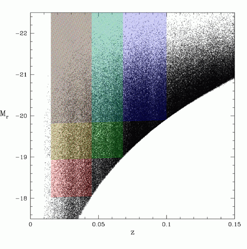
Figure 1.— Absolute $r$-band magnitude vs. redshift for galaxies in the SDSS redshift survey, highlighting the three volume-limited samples used for group identification. The three samples contain galaxies in the redshift ranges $0.015-0.1$, $0.015-0.068$, and $0.015-0.045$ and are complete for galaxies with r-band absolute magnitudes brighter than $-19.9$, $-19$, and $-18$, correspondingly. The absolute magnitude threshold for a given volume-limited sample evolves with redshift in order to account for passive luminosity evolution of the galaxy population.

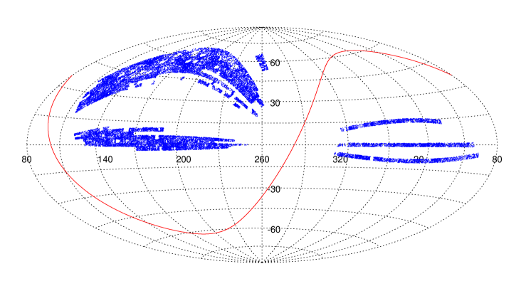
Figure 2.— Hammer (equal area) projection (in equatorial coordinates) of the SDSS volume-limited sample that goes out to redshift $0.1$. Points represent galaxies in the sample. The solid curve shows the location of the Galactic plane.

We construct three such volume-limited samples. Figure 1 shows these samples in the luminosity-redshift plane. Each dot in the figure shows a galaxy in the SDSS redshift survey. The sharp cutoff curve along the lower-right part of the plot shows our $r=17.5$ apparent magnitude limit. We select three redshift ranges for our volume-limited samples: $0.015-0.1$, $0.015-0.068$, and $0.015-0.045$. These samples are complete down to absolute $r$-band magnitudes of $M_{{}^{0.1}\!{r}}<-19.9$, $-19$, and $-18$, respectively. We refer to these samples as $Mr20$, $Mr19$, and $Mr18$, henceforth. Regions of the plot that make it into these three samples are shown in blue, green, and red, respectively. The limiting absolute magnitude of each sample changes slightly with redshift due to the passive evolution corrections applied to galaxy luminosities: as a galaxy is moved to the outer edge of a given volume-limited sample, its luminosity increases somewhat, allowing lower redshift galaxies to make it into the sample at lower luminosities than they do at higher redshifts. We choose the first limiting redshift of $z_{\mathrm{max}}=0.1$ because this yields the largest possible volume-limited sample (largest number of galaxies). We choose lower redshift samples in order to probe galaxy populations less luminous than $L_{\ast}$. We use a lower redshift limit of $0.015$ for all three samples to alleviate some of the problems associated with obtaining accurate photometry of nearby highly extended galaxies. The redshift limits, luminosity thresholds at $z_{\mathrm{max}}$, number of galaxies, and space densities of these samples are listed in Table 1.

Figure 2 shows a Hammer (equal area) projection (in equatorial coordinates) of sample $Mr20$. Points represent galaxies in the sample. The curve shows the location of the Galactic plane. The figure illustrates the patchy and non-uniform nature of the sample footprint on the sky, which has irregular edges, as well as multiple holes. This irregularity exacerbates systematic errors due to edge effects. We deal with incompleteness due to edge effects in § 5.

Figure 7 shows an equatorial slice through sample $Mr20$. The slice is $4^{\circ}$ thick and each point shows the RA and redshift of a galaxy in the sample. Prominent in this projection of the data is the the giant supercluster at $z\sim 0.08$ at the left end of the Sloan Great Wall of Galaxies, which extends from longitude 132 degrees (at $z\sim 0.05$) to longitude 210 degrees (at $z\sim 0.08$) (See gott_etal_05).

3. Mock Catalogs

Our main scientific motivation for constructing group catalogs from the SDSS data requires that identified groups most closely resemble systems of galaxies that occupy a common dark matter halo. Moreover, it is important that we statistically quantify the degree to which our groups do not satisfy this criterion. For both these reasons, it is imperative that we use mock galaxy catalogs that are constructed by populating dark matter halos in N-body simulations with mock galaxies. The N-body simulations must satisfy two basic conditions: they must contain a large enough volume to fit our largest volume-limited sample, $Mr20$, and they must resolve the smallest mass halos that can host a galaxy in our least luminous volume-limited sample, $Mr18$. HOD fits to the SDSS two-point correlation function of galaxies suggest that the minimum dark matter halo mass that can host a galaxy of luminosity $M_{{}^{0.1}\!{r}}\sim-18$ is approximately $2\times 10^{11}h^{-1}M_{\odot}$ (zehavi_etal_05; tinker_etal_05). Requiring that a halo contain at least forty dark matter particles to be resolved means that we need N-body simulations with particle masses less than $5\times 10^{9}h^{-1}M_{\odot}$.

We use a series of N-body simulations of a $\Lambda$CDM cosmological model, with $\Omega_{m}=0.3$, $\Omega_{\Lambda}=0.7$, $\Omega_{b}=0.04$, $h\equiv H_{0}/(100~{}\mathrm{km~{}s}^{-1}~{}\mathrm{Mpc}^{-1})=0.7$, $n_{s}=1.0$, and $\sigma_{8}=0.9$. This model is in good agreement with a wide variety of cosmological observations (see, e.g., spergel_etal_03; tegmark_etal_04b; abazajian_etal_05b). Initial conditions were set up using the transfer function calculated for this cosmological model by CMBFAST (seljak_zaldarriaga_96). The simulations were run at Los Alamos National Laboratory (LANL) using the Hashed-Oct-Tree (HOT) code (warren_Salmon_93). We use a total of six independent simulations of varying size and resolution, which we refer to as LANL1-6. The size of box $L_{\mathrm{box}}$, number of particles $N_{\mathrm{p}}$, and resulting particle mass $m_{\mathrm{p}}$ for each simulation are listed in Table 2. The gravitational force softening is $\epsilon_{\rm grav}=12h^{-1}\mathrm{kpc}$ (Plummer equivalent).

Table 2. Mock Catalog Parameters

	N-body				HOD
Mock	Name	$L_{\mathrm{box}}$	$N_{\mathrm{p}}$	$m_{\mathrm{p}}$	$M_{\mathrm{min}}$	$M_{\mathrm{cut}}$	$M_{1}$	$\alpha$
		($h^{-1}\mathrm{Mpc}$)		($10^{9}h^{-1}M_{\odot}$)	($10^{11}h^{-1}M_{\odot}$)	($10^{13}h^{-1}M_{\odot}$)	($10^{12}h^{-1}M_{\odot}$)
LANL1.Mr20	LANL1	$384$	$1024^{3}$	4.39	10.0	—	25.0	1.1
LANL1.Mr20b					9.08	1.14	12.3	0.9
LANL1.Mr19					3.7	—	8.2	1.0
LANL1.Mr18					1.9	—	3.4	0.9
LANL2.Mr20	LANL2	$384$	$1024^{3}$	4.39	10.0	—	25.0	1.1
LANL2.Mr20b					9.08	1.14	12.3	0.9
LANL2.Mr19					3.7	—	8.2	1.0
LANL2.Mr18					1.9	—	3.4	0.9
LANL3.Mr20	LANL3	$384$	$1024^{3}$	4.39	10.0	—	25.0	1.1
LANL3.Mr20b					9.08	1.14	12.3	0.9
LANL3.Mr19					3.7	—	8.2	1.0
LANL3.Mr18					1.9	—	3.4	0.9
LANL4.Mr20	LANL4	$400$	$1280^{3}$	2.54	10.0	—	25.0	1.1
LANL4.Mr20b					9.08	1.14	12.3	0.9
LANL4.Mr19					3.7	—	8.2	1.0
LANL4.Mr18					1.9	—	3.4	0.9
LANL5.Mr20	LANL5	$543$	$1024^{3}$	12.4	10.0	—	25.0	1.1
LANL5.Mr20b					9.08	1.14	12.3	0.9
LANL6.Mr20	LANL6	$768$	$1024^{3}$	35.1	10.0	—	25.0	1.1

We identify halos in the dark matter particle distributions using a friends-of-friends algorithm with a linking length equal to $0.2$ times the mean interparticle separation. We then populate these halos with galaxies using a simple model for the HOD of galaxies more luminous than a luminosity threshold. Every halo with a mass $M$ greater than a minimum mass $M_{\mathrm{min}}$ gets a central galaxy that is placed at the halo center of mass and is given the mean halo velocity. A number of satellite galaxies is then drawn from a Poisson distribution with mean $\left<N_{\mathrm{sat}}\right>=((M-M_{\mathrm{min}})/M_{1})^{\alpha}$, for $M\geq M_{\mathrm{min}}$. These satellite galaxies are assigned the positions and velocities of randomly selected dark matter particles within the halo. In order to construct mock catalogs for each of our three volume-limited samples $Mr20$, $Mr19$, and $Mr18$, we select sets of values for the parameters $M_{\mathrm{min}}$, $M_{1}$, and $\alpha$ that yield the observed zehavi_etal_05 galaxy-galaxy correlation functions for these samples. These HOD parameter values are similar to the best-fit values given by zehavi_etal_05 (they are slightly different because the model for $\left<N_{\mathrm{sat}}\right>$ was different in that paper). We refer to these sets of mock catalogs with the suffixes .Mr20, .Mr19, and .Mr18. In addition to these mock catalogs, we construct a set of catalogs for the $Mr20$ sample using an alternative HOD model, where the mean number of satellites in a halo of mass $M$ is $\left<N_{\mathrm{sat}}\right>=\mathrm{exp}[-M_{\mathrm{cut}}/(M-M_{\mathrm{min}})](M/M_{1})^{\alpha}$, for $M>M_{\mathrm{min}}$ (also used by tinker_etal_05). We fix the value of the slope $\alpha$ to 0.9, which is lower than that for the .Mr20 mocks, and we choose values for the remaining HOD parameters that yield the observed zehavi_etal_05 correlation function of $M_{{}^{0.1}\!{r}}<-20$ galaxies. We refer to these sets of mock catalogs with the suffix .Mr20b. The values for all mock HOD parameters are listed in Table 2. We construct ten realizations of each mock catalog listed in Table 2 by using different random number generator seeds when we (a) draw a number of satellite galaxies for each halo from a Poisson distribution of mean $\left<N_{\mathrm{sat}}\right>$, and (b) select random dark matter halo particles to give their positions and velocities to these satellite galaxies. The dispersion among the ten realizations for one mock catalog therefore represents the scatter among possible observed states for a given halo distribution and HOD model.

We now have a set of mock catalogs containing galaxies in real space and in the cubical geometry of the N-body simulations. We refer to these as our “real-space cube mocks”. We create a redshift-space version of these catalogs by assuming the distant observer approximation and aligning the line-of-sight along one of the axes of the simulation cubes. We use the mock galaxies’ peculiar velocities to move them along the line-of-sight into redshift space. We refer to the resulting mock catalogs as our “redshift-space cube mocks”. We use these real-space and redshift-space cube mocks to determine optimal parameters for our group-finding algorithm. We summarize this determination in §4 and discuss details in the Appendix.

For the purpose of studying the effects of SDSS incompleteness on our measured groups, as well as for obtaining estimates of the uncertainty in our measured group multiplicity function, we also require mock catalogs that have the same geometry as our SDSS volume-limited samples. The total volume of our largest sample, $Mr20$, is approximately $210^{3}h^{-3}{\mathrm{Mpc}}^{3}$, which is more than six times smaller than any of our mock cubes. However, the SDSS geometry is highly irregular (as seen in Fig. 2) and can only be fully embedded in a cube of much larger volume than the survey itself. The $Mr20$ sample, for example, has a maximum extent of $\sim 600h^{-1}\mathrm{Mpc}$ when both the North and South Galactic portions are included. In order to carve this sample geometry out of our mock catalogs, we create mock cubes with eight times larger volume by tiling each mock cube $2\times 2\times 2$. Since the N-body simulations used to construct the mocks were run with periodic boundary conditions, we can tile the cubes without having density discontinuities at the boundaries. We set the center of this tiled cube to be the origin and put galaxies into redshift space using the line-of-sight component of their peculiar velocities. We then compute RA, DEC, and redshift coordinates for every mock galaxy in the tiled cube. Finally, we only keep galaxies whose coordinates on the sky would place them in regions of the SDSS survey that have completeness greater than $90\%$, and whose redshifts lie within the redshift limits of the specific volume-limited sample we are constructing mock catalogs for.

Since the volume of each simulation cube is at least six times larger than our largest volume-limited sample $Mr20$, we try to carve out as many independent volumes with the $Mr20$ geometry as possible without too much overlap. We do this by performing many sets of three rotations (one around each Cartesian axis) and testing how much overlap the resulting catalogs have with each other (i.e., how many common mock galaxies do they share). With the right combination of rotation angles, we can carve out two $Mr20$ mock catalogs that share fewer than $3\%$ of their galaxies with each other, but we cannot obtain more without significant overlap. We create two such independent mock catalogs, with the correct SDSS geometry, from every one of the ten HOD realizations of the mock cubes listed in Table 2, except for the LANL6.Mr20 mock. This procedure yields 200 mock catalogs for the $Mr20$ sample (5 N-body simulations $\times$ 2 HOD models $\times$ 10 HOD realizations $\times$ 2 mocks per simulation cube), and 80 mock catalogs each for the $Mr19$ and $Mr18$ samples (4 N-body simulations $\times$ 1 HOD model $\times$ 10 HOD realizations $\times$ 2 mocks per simulation cube).

The final step in creating mock SDSS catalogs is to incorporate the fiber collision constraint. We use a friends-of-friends algorithm to identify groups of mock galaxies that are linked together by the $55^{\prime\prime}$ minimum angular separation of fibers. We then select “collided” mock galaxies (whose redshifts will be unknown) in each such collision group in a way that minimizes the number of such galaxies. For example, if a collision group contains three galaxies in a row, where the first is closer than $55^{\prime\prime}$ from the second and the second is closer than $55^{\prime\prime}$ from the third, but the first is more than $55^{\prime\prime}$ from the third, we will always select the middle galaxy to be the collided one. In cases where multiple choices yield the same number of collided galaxies, we select randomly (e.g., in collision groups with only two galaxies). This procedure is designed to mimic the tiling code that assigns spectroscopic fibers to SDSS target galaxies (blanton_etal_03a). If we perform this operation on the .Mr20 catalogs we end up with only $\sim 3\%$ of mock galaxies being tagged as collided. This is about half the fraction of SDSS galaxies in our $Mr20$ sample that don’t have measured redshifts due to fiber collisions. The reason for this discrepancy is that galaxies in the $Mr20$ volume-limited sample do not only collide with each other; they also collide with galaxies more luminous than $M_{{}^{0.1}\!{r}}\sim-20$ at redshifts higher than the sample limit $z=0.1$ and galaxies less luminous than $M_{{}^{0.1}\!{r}}\sim-20$ at lower redshifts. Most of these additional galaxies that can collide with a given galaxy in $Mr20$ are uncorrelated background or foreground galaxies. It is therefore sufficient to model them as a background screen of galaxies on the sky that have an angular correlation function equal to the mean for all SDSS galaxies. For this purpose, we use the very large volume LANL6.Mr20 cube mock. We use LANL6.Mr20 to construct a “screen” catalog with the correct SDSS angular geometry and a variable outer redshift limit, and superpose it onto each of our .Mr20, .Mr19, and .Mr18 mock catalogs. We then allow all galaxies to collide with each other and keep track of collided mock galaxies. We set the outer redshift limit of the screen catalog to the value that results in $\sim 6\%$ of mock galaxies being tagged as collided. We find that we need approximately seven times more galaxies in the screen catalog than in the mocks in order to achieve this collided fraction.

Using this approach we construct three versions of every mock catalog described above: a version with no fiber collisions applied (“true” version), a version where collided galaxies have no redshifts and are dropped out of the mock catalog altogether (“uncorrected” version), and a version where collided galaxies are assigned the redshift of the galaxy they collided with (“corrected” version). These mock catalogs allow us to test the effects of fiber collisions on our measured group multiplicity function (discussed in § 5.)

4. Group-Finding Algorithm

We wish to identify galaxy groups primarily in order to measure the group multiplicity function and use it to constrain the HOD of galaxies as a function of galaxy properties. This goal places a number of demands on the group-finding algorithm: (1) It should identify galaxy systems that occupy the same dark matter halos with the least possible merging of different halos into the same group and the least possible splitting of individual halos into multiple groups. (2) It should produce a group multiplicity function that is unbiased with respect to the halo multiplicity function. (3) It should be simple and well-defined so that the statistical and systematic uncertainty in the measured group multiplicity function can be accurately characterized. (4) It should use only the spatial positions of galaxies in redshift space to identify groups, and not galaxy properties such as color or luminosity. These requirements point to an algorithm that uniquely identifies density enhancements in redshift space.

We adopt the simple and well understood friends-of-friends (FoF) algorithm, where galaxies are recursively linked to other galaxies within a specified linking volume around each galaxy. The FoF algorithm has several attractive features. First, for a given linking volume (usually specified by one linking length in real space and two linking lengths in redshift space), FoF produces a unique group catalog. Second, it does not assume or enforce any particular geometry for groups (e.g., spherical), but rather identifies structures that are approximately enclosed by an isodensity surface whose density is monotonically related to the linking lengths. Third, the algorithm satisfies a nesting condition: all the members of a group identified with one set of linking lengths are also members of the same group identified using larger linking lengths.

The FoF algorithm has been used extensively to identify dark matter halos in N-body simulations (e.g., davis_etal_85) and has been shown to produce halo catalogs with mass functions that are close to universal (within $\sim 20\%$) for a wide range of epochs and cosmological models (jenkins_etal_01). FoF has also been the most used algorithm for identifying galaxy groups in redshift surveys (huchra_geller_82; geller_huchra_83; nolthenius_white_87; ramella_etal_89; moore_etal_93; ramella_etal_97; ramella_etal_99; tucker_etal_00; giuricin_etal_00; ramella_etal_02; merchan_zandivarez_02; eke_etal_04a), though alternative methods have also been used (see e.g., tully_87; marinoni_etal_02; gerke_etal_05; yang_etal_05). These FoF studies all used the same basic algorithm, but differed in their choices for linking lengths and in their methods for dealing with the varying density of galaxies inherent in flux-limited surveys.

We use the basic huchra_geller_82 algorithm, where two galaxies are linked to each other if both their transverse and line-of-sight separations are smaller than a given pair of projected and line-of-sight linking lengths, respectively. Specifically, two galaxies $i$ and $j$ with angular separation $\theta_{ij}$ and redshifts $z_{i}$ and $z_{j}$, have a projected separation $D_{\perp,ij}$ and a line-of-sight separation $D_{\parallel,ij}$ (both in $h^{-1}\mathrm{Mpc}$) given by

$$D_{\perp,ij} = (c/H_{0})(z_{i}+z_{j})~{}\mathrm{sin}(\theta_{ij}/2),$$ (1)

$$D_{\parallel,ij} = (c/H_{0})|z_{i}-z_{j}|.$$ (2)

The two galaxies are then linked to each other if

$$D_{\perp,ij}\leq b_{\perp}~{}\bar{n}_{\mathrm{g}}^{-1/3}$$ (3)

and

$$D_{\parallel,ij}\leq b_{\parallel}~{}\bar{n}_{\mathrm{g}}^{-1/3},$$ (4)

where $\bar{n}_{\mathrm{g}}$ is the mean number density of galaxies, and $b_{\perp}$ and $b_{\parallel}$ are the projected and line-of-sight linking lengths in units of the mean intergalaxy separation. Since we use volume-limited samples of SDSS galaxies, $\bar{n}_{\mathrm{g}}$ is constant throughout the sample volumes, and thus the linking lengths are also constant.

The resulting linking volume around each galaxy is very similar to a cylinder, oriented along the line-of-sight, whose radius is equal to the projected linking length and whose height is equal to twice the line-of-sight linking length. It is not a perfect cylinder because its radius increases with redshift, making it slightly wider at the far end than at the near end, and its bases are slightly curved. However, for the small linking lengths considered here, a cylinder is a good approximation. The FoF algorithm works recursively, whereby a galaxy is linked to all its “friends”, which are in turn linked to their “friends”, etc., to yield a unique group of galaxies.

4.1. Choice of Linking Lengths

The most important ingredient of our group-finding algorithm is our choice for the linking lengths $b_{\perp}$ and $b_{\parallel}$. If the linking lengths are too small, then the group-finder will break up single halos into multiple groups. If the linking lengths are too large, then different halos will be fused together into single groups. There are no values for the linking lengths that will work perfectly for every halo, even in real space. In redshift space this problem becomes substantially worse, since redshift-space distortions both move halos and elongate them along the line-of-sight, often causing them to overlap with each other. The right choice of linking lengths depends on the purpose for which groups are being identified. If we require a group catalog that is highly inclusive and groups together every galaxy inhabiting the same halo, then we will use larger linking lengths than if our goal is to minimize contamination by galaxies that come from different halos. For our purposes, we wish to obtain a balance between being inclusive and reducing contamination, while producing groups that have an unbiased multiplicity function.

In order to find the right combination of linking lengths, we use the mock galaxy catalogs described in § 3. Specifically, we use the real- and redshift-space cube mocks, which are constructed by applying simple HOD models to the LANL1 and LANL4 N-body simulations. Since we know which mock galaxies occupy the same dark matter halos, we can evaluate how well a particular choice of linking lengths recovers features of the halo population. The mocks that we use here have a cubical geometry, and we assume the distant observer approximation when we put mock galaxies into redshift space. We use the full cubical mocks rather than those with the correct SDSS geometry because the full mocks have a much larger volume and thus better statistics. Moreover, our goal is to find the best linking lengths for any redshift survey, and we will deal with systematic effects specific to our SDSS sample geometry separately. The FoF algorithm that we use is therefore slightly different from the one outlined above, in that the linking volume is a perfect cylinder (i.e., $D_{\perp,ij}$ is simply the projected distance between two mock galaxies).

We run the FoF group-finder on the mock catalogs for a grid of linking length values, and we study the properties of the resulting group catalogs. Specifically, we investigate four features of the recovered group distribution: (1) the group multiplicity function compared to the “true” halo multiplicity function; (2) The relation between the number of galaxies in a halo $N_{\mathrm{true}}$ and the number of galaxies in its associated group $N_{\mathrm{obs}}$; (3) The distribution of projected group sizes as a function of group richness compared to the “true” distribution of projected halo sizes as a function of halo multiplicity; (4) The distribution of group velocity dispersions as a function of group richness compared to the “true” distribution of halo velocity dispersions as a function of halo multiplicity.

We check how each set of linking lengths performs in the above four tests, for each of the four HOD model mock cubes (.Mr20, .Mr20b, .Mr19, .Mr18). In the case of each HOD model, we average results over the 10 HOD realizations described in § 3 and over the LANL1 and LANL4 N-body simulations. We do this procedure for groups that are identified in both real space (for which there is only one linking length), and redshift space. These tests are described in detail in the Appendix. Here we summarize the main results.

In real space, a linking length choice of $b=0.2$ yields galaxy groups with ten or more members that pass all four tests listed above. Groups with $N<10$ show systematic deviations in abundance, multiplicity, projected sizes, and velocity dispersions from the corresponding halos with $N<10$. The choice of $b=0.2$ is not surprising, given that the same linking length was used to identify halos in the N-body simulations. It is also not surprising that the group-finding fails the tests for small groups, where adding or losing a couple of galaxies makes a large fractional difference to the group size. The threshold of $N\sim 10$ is independent of the underlying dark matter halo mass. This means that we can push the regime in which the groups are reliable to lower mass systems by using a lower luminosity sample (where each halo will contain more galaxies). Of course, the change of luminosity threshold comes at the expense of statistical power, since low luminosity samples have smaller volumes than high luminosity samples. The number of groups in a volume-limited sample scales roughly with the number of galaxies, and a luminosity threshold near the characteristic luminosity $L_{*}$ maximizes this number.

In redshift space the situation is more complicated. No set of transverse and line-of-sight linking lengths is able to produce groups that pass all four tests listed above, even for large size groups. Figure 3 summarizes our tests for the .Mr20 HOD model mocks. Results for the other HOD models are similar and are shown in the Appendix. The figure shows regions (shaded) of the two-dimensional linking length space ($b_{\parallel}$ vs. $b_{\perp}$) that pass each of our four tests.

4.1.1 Multiplicity Function

The dark and thin shaded region in Figure 3, labeled $n(N)$, shows linking lengths that pass the group multiplicity function test. In other words, these linking lengths yield mock group catalogs whose multiplicity functions are unbiased relative to the “true” input halo multiplicity function, in the regime $N\geq 10$. In this case, “unbiased” means that the shape of the multiplicity function is on average the same as the “true” shape and its amplitude is within $10\%$ of the “true” amplitude. Linking length values that lie along the upper boundary of the shaded region (e.g, the values $b_{\perp}=0.11$, $b_{\parallel}=1.5$) yield multiplicity functions that are $10\%$ too high in amplitude, whereas values that lie along the lower boundary yield multiplicity functions whose amplitudes are $10\%$ too low. These results show that an increase in either linking length generally leads to an increase in the multiplicity function for $N\geq 10$. This increase is compensated for by a corresponding decrease in the abundance of isolated (i.e., $N=1$) and low $N$ groups. The shaded region appears to be close to horizontal only because the vertical axis is highly compressed with respect to the horizontal axis.

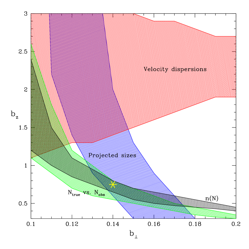
Figure 3.— Regions of the FoF linking length parameter space that do well in recovering galaxy groups that have similar properties to their parent halos. Each shaded region shows the combination of perpendicular and line-of-sight FoF linking lengths that are successful in recovering a particular feature of the group distribution, measured using mock galaxy catalogs. The four features are: (a) the group multiplicity function (black region); (b) the relation between halo and group richness for halos and groups that are matched one-to-one (green region); (c) the projected sizes of groups as a function of group richness (blue region); (d) the line-of-sight velocity dispersion of groups as a function of group richness (red region). The yellow star denotes the FoF parameters that we apply to identify groups in the SDSS.

4.1.2 $N_{\mathrm{true}}$ vs. $N_{\mathrm{obs}}$

The group multiplicity function is an average statistic showing the abundance of all groups as a function of $N$. It is therefore possible, in principle, for it to be unbiased relative to the halo multiplicity function, without the relation between individual halo multiplicities and their recovered group multiplicities being correct. For this reason, we also require that the group-finder yield an unbiased relation between the multiplicity of individual halos, $N_{\mathrm{true}}$, and their recovered groups, $N_{\mathrm{obs}}$. In order to check this, we must match input halos to recovered groups in a one-to-one way. There are many ways to do this matching, and no one way is more correct than another. For example, a halo can be associated with the group that contains most of its galaxies, or the group that contains its central galaxy, or the group whose centroid is closest to the halo center. We associate each halo to the group that contains its central galaxy. When two or more halos are matched to the same group, we choose the halo that shares the largest number of common galaxies with the group. Halos that are not associated with any group are considered “undetected,” and groups that are not associated with any halo (because they don’t contain any halo central galaxies) are considered “spurious”.

The light (and green) shaded region in Figure 3 that roughly tracks and is slightly wider than the $n(N)$ region shows linking lengths that pass the $N_{\mathrm{true}}$ vs. $N_{\mathrm{obs}}$ test. In other words, these linking lengths yield mock group catalogs with an unbiased median relation between $N_{\mathrm{true}}$ and $N_{\mathrm{obs}}$ for associated halos and groups, in the regime $N\geq 10$. We consider the relation to be unbiased if its slope is within $10\%$ of unity. Linking length values that lie along the upper boundary of the shaded region yield associated halos and groups with a median relation $N_{\mathrm{true}}=1.1N_{\mathrm{obs}}$, whereas values that lie along the lower boundary yield the relation $N_{\mathrm{true}}=0.9N_{\mathrm{obs}}$. As expected, most linking lengths that pass the multiplicity function test also pass the $N_{\mathrm{true}}$ vs. $N_{\mathrm{obs}}$ test. This breaks down, however, for values of $b_{\perp}$ greater than 0.16-0.17.

4.1.3 Projected Sizes

The (blue) shaded region in Figure 3, labeled “Projected sizes”, shows linking lengths that pass the projected sizes test. These linking lengths yield mock groups with an unbiased median relation between rms projected size and group multiplicity $N$, in the regime $N\geq 10$. We consider the relation to be unbiased if it is within $10\%$ of the “true” relation between median rms projected halo size and halo multiplicity. This shaded region is roughly vertically oriented because the projected linking length $b_{\perp}$ affects the projected sizes of groups much more than the line-of-sight linking length $b_{\parallel}$. Clearly, increasing $b_{\perp}$ leads to galaxy groups with larger projected sizes. The shaded region is not completely vertical, however, because increasing $b_{\parallel}$ also leads to larger projected size groups, albeit in a much less sensitive way.

4.1.4 Velocity Dispersions

The (red) shaded region in Figure 3, labeled “Velocity dispersions”, shows linking lengths that pass the velocity dispersion test. These linking lengths yield mock groups with an unbiased median relation between group velocity dispersion and group multiplicity $N$, in the regime $N\geq 10$. We consider the relation to be unbiased if it is within $10\%$ of the “true” relation between median halo velocity dispersion and halo multiplicity. This shaded region is roughly horizontally oriented because the line-of-sight linking length $b_{\parallel}$ affects the velocity dispersions of groups much more than $b_{\perp}$. Clearly, increasing $b_{\parallel}$ leads to galaxy groups with larger velocity dispersions. The shaded region is not completely horizontal, because changing $b_{\perp}$ also affects the velocity dispersions of groups, though not consistently in the same sense.

4.1.5 Our Adopted Linking Lengths

It is obvious from Figure 3 that no combination of FoF linking lengths passes all four tests listed above. We can choose linking lengths that successfully recover the abundance and projected sizes, or the abundance and velocity dispersions of groups as a function of multiplicity, but not all three simultaneously. We can also choose linking lengths that successfully recover both the projected sizes and velocity dispersions of groups as a function of multiplicity, but since the multiplicity function of such groups is incorrect, the overall size and velocity dispersion distributions will also be incorrect. This failure to recover all features of groups in redshift space is a fundamental shortcoming of the FoF group-finder when applied to redshift space. Given that most redshift-space group-finding algorithms operate on very similar principles, i.e., they identify overdense regions that are elongated along the line-of-sight, it is likely that this shortcoming is shared by other group-finders as well. To our knowledge, no group-finder has been shown to pass all four of the tests considered here for a single choice of parameters.

Figure 3 shows that in order to recover groups with unbiased velocity dispersions, the line-of-sight linking length must be substantially larger than the mean intergalaxy separation. With $b_{\parallel}$ that large, groups are bound to be linked together along the line-of-sight. The only way to then obtain groups with the correct multiplicity function is to have a transverse linking length small enough that galaxies in the outer parts of halos are not included in the recovered groups. The resulting groups bear little physical resemblance to their parent halos. If, on the other hand, we recover groups with unbiased projected sizes, then the groups will be missing some of their fastest moving galaxies and this decrease in multiplicity will be compensated by including as group members a few galaxies in the infall regions of halos. These groups are much more physically similar to their parent halos. For this reason, we choose to sacrifice velocity dispersions, rather than projected sizes, when selecting values for the FoF linking lengths.

Figure 3 shows the linking length values that we adopt and use in this paper (yellow star). These values are

$$b_{\perp}=0.14,\qquad b_{\parallel}=0.75~{}.$$ (5)

Our mock catalog tests show that the FoF algorithm with these linking lengths finds galaxy groups with $N\geq 10$ that have: (1) an unbiased multiplicity function; (2) an unbiased median relation between the multiplicities of groups and their associated halos; (3) a spurious group fraction of less than $\sim 1\%$; (4) a halo completeness (fraction of halos that are associated one-to-one with groups) of more than $\sim 97\%$; (5) the correct projected size distribution as a function of multiplicity; (6) a velocity dispersion distribution that is $\sim 20\%$ too low at all multiplicities. These results hold for all of the mock catalogs that we have used (see results for other HOD models in the Appendix) and are thus not very sensitive to the HOD model assumed or to the specific realization of the underlying density field. We note that our adopted group-finder only has the above properties when dark matter halos are defined using a FoF algorithm with a linking length of 0.2 times the mean interparticle separation, since that was the definition used to construct our mock catalogs. A different halo definition (such as FoF using a different linking length, or a spherical overdensity halo-finder) will result in a different optimal group-finder.

Previous FoF group analyses have used different linking lengths. For example, eke_etal_04a adopt $b_{\perp}=0.13,b_{\parallel}=1.43$ in their analysis of groups in the 2dF Galaxy Redshift Survey (2dFGRS; colless_etal_01). With a similar transverse linking length but much larger line-of-sight linking length than used here, this parameter combination yields unbiased projected sizes and velocity dispersions, but it overpredicts the abundances of halos by $20-30\%$ at large multiplicities (see Figure 3). These groups are thus poorly suited to our primary objective of using group abundances as a cosmological test. yang_etal_05 and weinmann_etal_05 use a group-finder that assumes a mass, radius, and velocity dispersion for each preliminary group and then includes or discards galaxies from the group based on these assumed properties (similar to a matched filter technique). This method might, in principle, be able to simultaneously recover groups with unbiased abundances, projected sizes, and velocity dispersions - at the expense of model independence - but this remains to be tested.

5. Incompleteness

There are two main sources of incompleteness that will affect the richnesses of groups, and hence the multiplicity function, in our SDSS group catalogs: fiber collisions and survey edges. Both these effects will prevent galaxies from being included in some groups, and thus cause the richness of these groups to be underestimated. These sources of incompleteness and their effects on the measured group multiplicity function must be accounted for.

5.1. Fiber Collisions

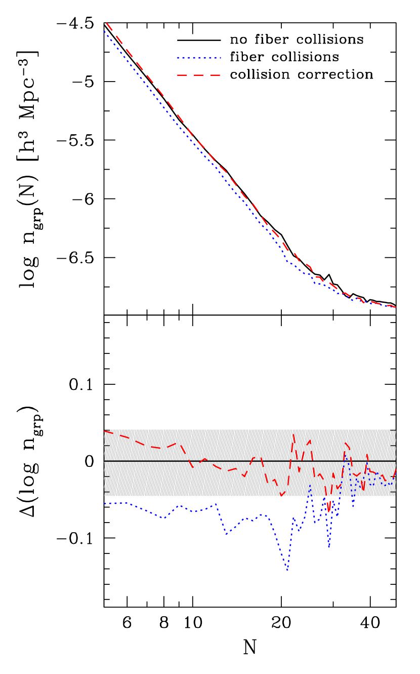
Figure 4.— Effect of fiber collisions on the group multiplicity function measured using mock SDSS galaxy catalogs, which are described in § 3. The top panel shows the differential group multiplicity function for mock catalogs that contain no fiber collisions and thus represent the “true” case (solid black curve), that lose galaxies due to fiber collisions as in the SDSS survey (dotted blue curve), and that are corrected for fiber collisions as described in § 5 (dashed red curve). The bottom panel shows the ratio of each case to the “true” one. The shaded region encloses $\pm 10\%$ deviations from the “true” multiplicity function. These results are averaged over all of our .Mr20 mock catalogs.

Fiber collisions cause an incompleteness that grows with the surface density of galaxies and is thus especially important in group and cluster studies. Moreover, the surface density in groups is likely a function of group richness. The mean surface density of a group of richness $N$, mass $M$, and radius $R$ scales like $\Sigma\sim N/R^{2}\sim N/M^{2/3}$. For a power-law relation between mean richness and halo mass $N\sim M^{\alpha}$, the surface density is $\Sigma\sim N^{1-2/3\alpha}$. This scaling relation is clearly a crude approximation, but it illustrates that the incompleteness due to fiber collisions likely varies with group richness and can thus affect both the amplitude and slope of the multiplicity function.

We use the 100 LANL1-5.Mr20 mock catalogs (5 N-body simulations $\times$ 10 HOD realizations $\times$ 2 mocks per simulation cube) to assess the impact of fiber collisions on the group multiplicity function. We apply the group-finder described in § 4 to the “uncorrected” and “true” versions of these mock catalogs and measure the resulting multiplicity functions. Figure 4 shows these multiplicity functions averaged over all the mock catalogs. The figure shows that dropping collided galaxies from the sample lowers the amplitude of the multiplicity function by more than 10% and also slightly changes its slope. The amplitude drops because some groups in each richness bin lose galaxies and are thus shifted to lower $N$ bins. There are also some groups from higher $N$ bins that are shifted into these bins, but their number is smaller than the number of groups lost because the abundance of groups drops steeply with increasing $N$.

zehavi_etal_05 show that the effect of fiber collisions on the galaxy two-point correlation function can be successfully corrected for by including each collided galaxy at the redshift of its nearest neighbor. We apply the same correction to our mock catalogs to produce a set of “corrected” mocks. Figure 4 shows that this correction works very well in the regime $N\geq 10$, and we therefore adopt it for our group identification.

Figure 5.— Fraction of groups affected by survey edges, measured using mock SDSS galaxy catalogs (described in § 3). Groups are considered affected by edges if they lose any galaxies that would have been included in the absence of edges. The panels show the edge fraction of groups in bins of the distance from their centroids to the closest edge $r_{\mathrm{edge}}$ (left panel) and group richness $N$ (right panel). The right panel also shows the fraction of groups that lose more than $25\%$ of their member galaxies due to edges (dashed curve). These results are averaged over four independent .Mr20 mock catalogs.

5.2. Survey Edges

Groups that are identified near the edges of a given sample could be missing galaxies that are located just outside the sample. Similar to fiber collisions, edge effects always shift groups from higher to lower richness. Moreover, large and extended groups have a higher probability of being affected by edges than do small and compact groups because they can straddle an edge while being further away from it. Edge effects are most severe when the ratio of a sample’s surface area to its enclosed volume is high. Figure 2 shows that the SDSS sample has a highly irregular footprint on the sky, which implies a high surface-to-volume ratio. Edge effects are, therefore, potentially severe in our samples. When the SDSS survey is complete and the gap in the North Galactic cap is filled in, edge effects will be much less important.

We can measure the effects of edges using our mock catalogs, since we know what galaxies lie on the other side of edges. For every group identified in our LANL1-5.Mr20 mock catalogs, we determine how many galaxies are missing due to edges. An edge can lie either in the perpendicular direction, or along the line-of-sight due to a sample’s redshift limits.

The solid curve in the right panel of Figure 5 shows the fraction of mock groups that are missing one or more galaxies due to edges, as a function of group richness $N$. The affected fraction climbs from 10% to 40% as $N$ goes from 5 to 50. Edges clearly affect a large fraction of high richness groups in our sample, but counting a group as affected if it loses only a single galaxy is a very conservative test. It makes more sense to calculate the fraction of groups that lose a fixed fraction of their galaxies, rather than just a single galaxy. The dashed curve in the same panel shows the fraction of groups that lose 25% or more of their galaxies. The affected fraction defined this way is $\sim 10\%$, roughly independent of richness. Figure 6 shows the effect of edges on the multiplicity function (blue curve). The effect of edges on the abundance of mock groups grows from zero at $N=2$ to approximately 20% at $N=50$. It is, therefore, very important to correct for edges, since they systematically change the shape of the multiplicity function and, hence, the derived HOD.

We measure the shortest distance of every galaxy from the survey edges by laying down points around each galaxy at successively larger radii and checking if they also lie within our sample volume. The smallest radius at which points fall outside the sample volume is the distance of the galaxy from the edge. Any group that contains at least one galaxy within a linking length from the edge, whether it is a projected linking length in the tangential direction or a line-of-sight linking length in the redshift direction, is potentially affected, since there could be galaxies on the other side that would be linked to the same group. One possible way to deal with edges is to throw out all such groups. This is a very conservative solution, since it ensures that all groups in our final sample are uncontaminated by edges. However, it is tricky to estimate the new effective volume of the sample, which is necessary for measuring the multiplicity function. Moreover, the effective volume for large groups will be smaller than that for small groups. Another possibility is to keep all groups, but somehow correct the multiplicities of those that are potentially affected by edges. This solution has the advantage that no groups are lost, but it is once again difficult to estimate the effective volume of the sample, even if all multiplicity corrections are exactly right. A third possibility is to reject all groups whose centers lie less than a minimum distance from the edge. This correction has the advantage that it produces an unbiased sample and it is simple to estimate the new effective volume. However, it is important to use the correct minimum distance. If it is too small, then the correction will not work for the largest groups; if it is too big, then we will unnecessarily reduce our sample size.

The left panel of Figure 5 shows the fraction of mock groups that are missing one or more galaxies due to edges, as a function of the distance from the group centroid to the edge. The fraction drops from 20% at 100 Kpc to 5% at 500 Kpc and less than 1% at 1 Mpc. It does not go to zero at larger distance because there are groups with high velocity dispersion that can be far from the edge and still have galaxies within a linking length of the outer or lower redshift limit of our sample. This figure suggests that if we set the minimum distance to 500 Kpc in the tangential direction and 500 km/s in the redshift direction, we should eliminate most groups that are affected by edges. We make this correction on our mock group catalogs, and the number of groups in the resulting catalog is reduced by $\sim 22\%$ on average. We estimate the new effective volume of each group catalog by scaling the original volume by the fraction of groups that survive the edge cut. This estimate, though not exactly accurate, is simple to make and adequate for our purposes. Figure 6 shows that this correction results in a multiplicity function that is unbiased due to edges (dashed red curve).

Our mock catalog tests show that we can deal with survey edges effectively if we measure the multiplicity function after eliminating all groups whose centers (estimated as the centroids of their member galaxy positions) lie less than 500 Kpc from an edge in the tangential direction or less than 500 km/s from an edge in the radial direction. Applying this edge cut to the $Mr20$, $Mr19$, and $Mr18$ SDSS group catalogs reduces the numbers of groups by 22.0%, 30.2%, and 41.1%, respectively. Our measurement of the multiplicity function for these samples includes this correction, though the group catalogs that we present include all groups.

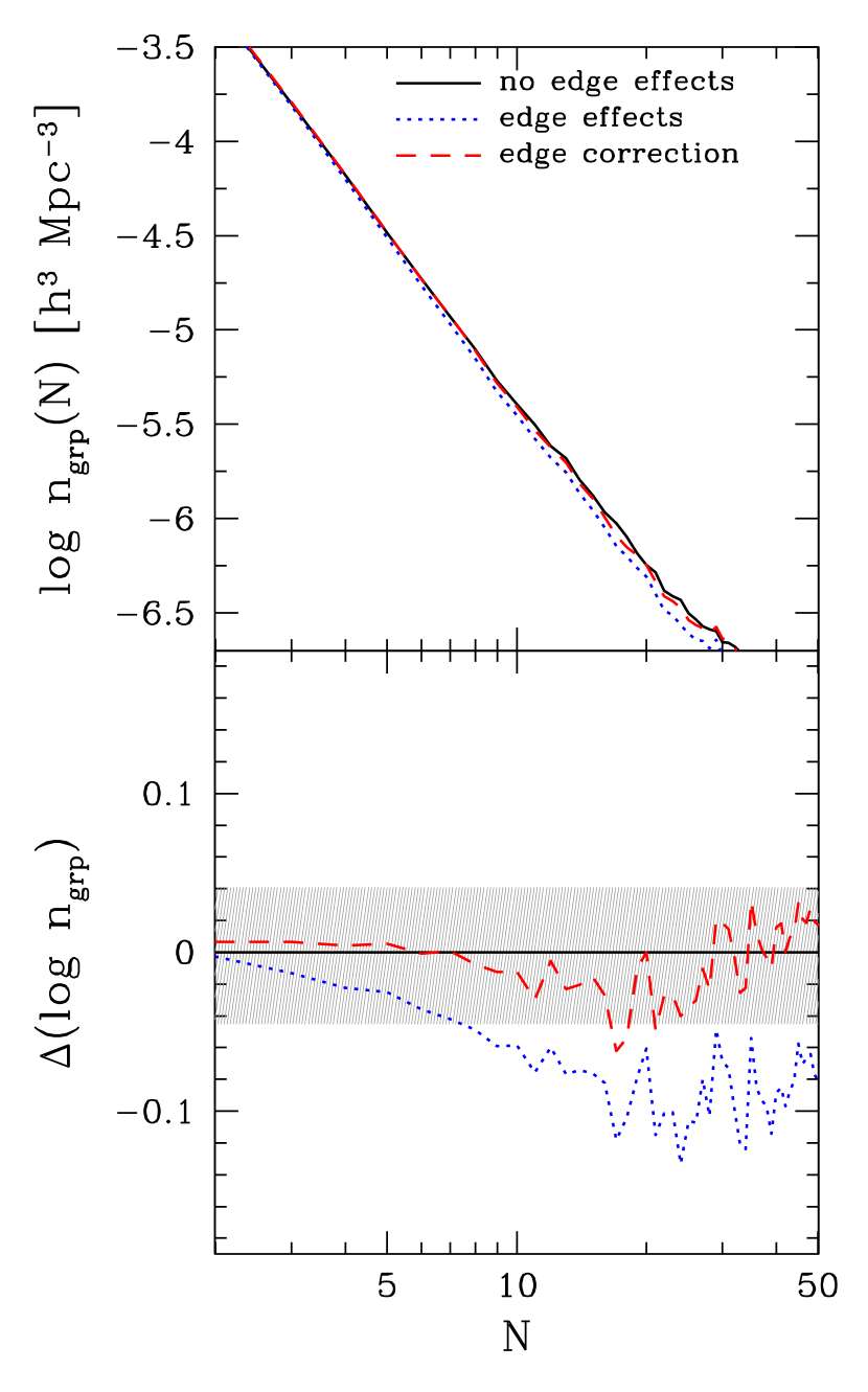
Figure 6.— Effect of survey edges on the group multiplicity function measured using mock SDSS galaxy catalogs (described in § 3). The figure shows the group multiplicity function for mock catalogs that contain no edge effects and thus represent the “true” case (solid black curve), that contain edge effects as in the SDSS survey (dotted blue curve), and that are corrected for edge effects as described in § 5 (dashed red curve). All other features as in Fig. 4. These results are averaged over all of our .Mr20 mock catalogs.

6. Group and Cluster Catalog

We apply our group-finding algorithm to the three volume-limited samples described in § 2 and get three group catalogs. The fractions of ungrouped, isolated galaxies are 43.7%, 41.2%, and 39.8% for the $Mr20$, $Mr19$, and $Mr18$ samples, respectively. The fractions of galaxies grouped in pairs are 19.1%, 18.3%, and 17.9%. The remaining 37.2%, 40.6%, and 42.3% of galaxies are in groups of three or more members. Samples $Mr20$, $Mr19$, and $Mr18$ contain a total of 4107, 2684, and 1357 groups with richness $N\geq 3$, respectively.

Figure 8 shows an equatorial slice with groups identified from sample $Mr20$. The slice is $4^{\circ}$ thick and each point shows the RA and redshift of a group with $N\geq 3$. A comparison of this figure to Figure 7 shows that groups and clusters trace the large-scale structure of galaxies, as expected. Larger groups are preferentially located in higher density regions, whereas smaller groups are more uniformly distributed. It is striking that the majority of very large groups reside within the large supercluster at $z=0.08$. Figure 9 shows the same slice, but with points representing the positions of member galaxies in $N\geq 3$ groups. A visual inspection of the figure shows that group velocity dispersions, which are responsible for the finger-of-God effect, are largest in the most luminous groups.

For each group, we compute an unweighted group centroid, which consists of a group right ascension, declination, and mean redshift. We compute a total group luminosity that is the sum of luminosities of its member galaxies. Since we are dealing with volume-limited samples, the luminosity of a given group in samples $Mr20$, $Mr19$, $Mr18$, only counts galaxies with absolute magnitudes brighter than -19.9, -19, -18, respectively. For example, for the $Mr20$ sample, the total group absolute magnitude is

$$M_{r20}=-2.5\mathrm{log}\left(\sum_{i=1}^{N}10^{-0.4M_{{}^{0.1}\!{r},i}}\right),$$ (6)

and it is equivalent to integrating the galaxy luminosity function within the group from $M_{{}^{0.1}\!{r}}=-19.9$ to $-\infty$. Note that we compute these group absolute magnitudes using the altered absolute magnitudes for galaxies that do not have measured redshifts due to fiber collisions (see § 2). We also compute a total group color, which is simply defined as $(g-r)_{20}=M_{g20}-M_{r20}$. We compute a group one-dimensional velocity dispersion given by

$$\sigma_{v}=\frac{1}{1+\bar{z}}\sqrt{\frac{1}{N-1}\sum_{i=1}^{N}(cz_{i}-c\bar{z})^{2}},$$ (7)

and an rms projected group radius given by

$$R_{\perp,\mathrm{rms}}=\sqrt{\frac{1}{N}\sum_{i=1}^{N}r_{i}^{2}},$$ (8)

where $r_{i}$ is the projected distance between each member galaxy and the group centroid.

In the three portions of Table 3, we present the groups and clusters with $N\geq 3$, selected from samples $Mr20$, $Mr19$, and $Mr18$. For each group, we list a group ID (column 1); the (J2000) right ascension and declination of the group centroid (columns 2, 3); the mean redshift of the cluster (column 4); the group richness $N$ (column 5); the total $r$-band absolute magnitude of the group, $M_{r20}$ (column 6); the total color of the group, $(g-r)_{20}$ (column 7); the line-of-sight velocity dispersion of the group, $\sigma_{v}$ (column 8); the projected rms radius of the group $R_{\perp,\mathrm{rms}}$ (column 9); the perpendicular distance of the group center from the survey edge $r_{\mathrm{edge}}$ (column 10). The groups in each portion of Table 3 are ranked in decreasing order of richness $N$. We show the first few rows of each portion of the table in the text and make the entire table available in the electronic version of the journal, as well as at http://cosmo.nyu.edu/aberlind/Groups.

In Table 4, we present the member galaxies of the groups listed in Table 3. For each galaxy we list the ID of the group to which it belongs (column 1); the (J2000) right ascension and declination (columns 2, 3); the redshift (column 4); the $r$-band absolute magnitude $M_{{}^{0.1}\!{r}}$ (column 5); the ${}^{0.1}\!{(g-r)}$ color (column 6); a fiber collision flag that is equal to 0 if the galaxy has its own measured redshift and 1 if it has been given the redshift of its nearest neighbor (column 7); the perpendicular distance of the galaxy from the survey edge $r_{\mathrm{edge}}$ (column 8). As before, we show the first few rows of each portion of Table 4 in the text and make the entire table available in the electronic version of the journal, as well as at http://cosmo.nyu.edu/aberlind/Groups.

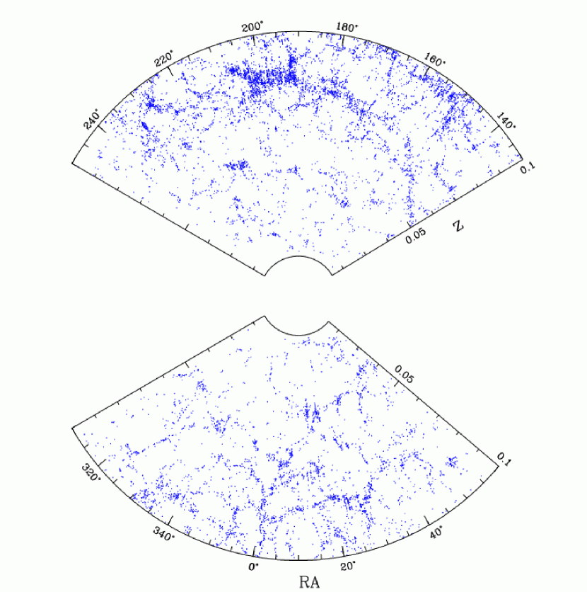
Figure 7.— Equatorial slice through the SDSS volume-limited sample in the redshift range $0.015-0.1$. The slice is $4^{\circ}$ thick and each point shows the RA and redshift of a galaxy in the sample.

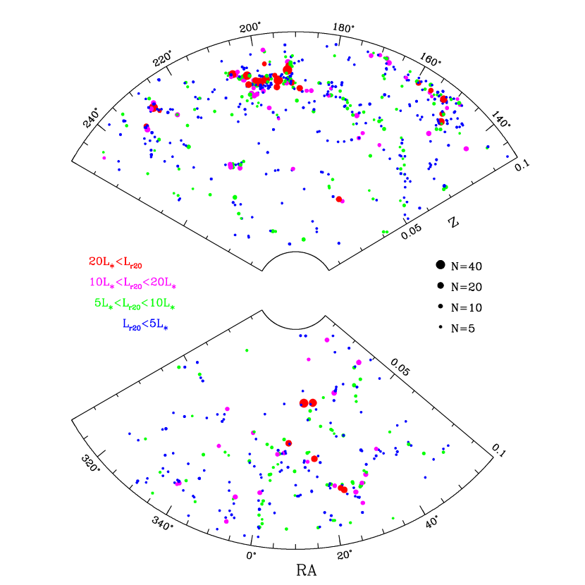
Figure 8.— $4^{\circ}$ thick equatorial slice showing galaxy groups in the $Mr20$ volume-limited sample. Each point shows the location of a group of richness $N\geq 3$. Points have a size proportional to group richness $N$ and a color encoding according to their total $r$-band luminosity $L_{r20}$ (defined in the text) in units of $L_{\ast}$ (where we adopt $M_{\ast}=-20.44$), as listed in the legend.

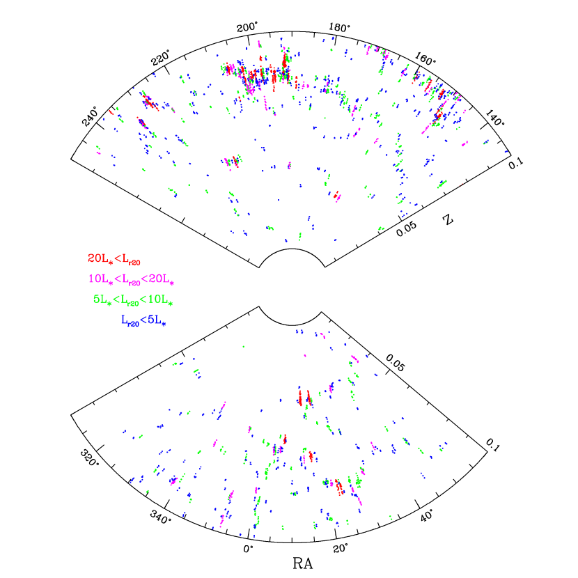
Figure 9.— Same as Fig. 8 except that points show the locations of member galaxies in groups of richness $N\geq 3$.

Table 3. Group and Cluster Catalogs for Samples $Mr20$, $Mr19$, and $Mr18$

ID	RA	DEC	$\bar{z}$	$N$	$M_{r20}$	$(g-r)_{20}$	$\sigma_{v}$	$R_{\perp,\mathrm{rms}}$	$r_{\mathrm{edge}}$
	(deg)	(deg)					(km/s)	($h^{-1}\mathrm{Mpc}$)	($h^{-1}\mathrm{Mpc}$)
$Mr20$
33974	239.580740	27.312343	0.08797	132	-25.920	0.946	723.7	1.371	17.7
16089	247.172589	40.164633	0.03057	97	-25.468	0.891	661.1	1.318	89.3
8817	358.535971	-10.372017	0.07405	61	-25.190	0.921	736.0	0.734	17.9
14552	183.450292	59.266666	0.09386	51	-24.861	0.808	338.3	1.079	22.9
12289	159.824898	4.987457	0.06815	51	-24.859	0.899	661.4	1.161	47.1
3025	195.700154	-2.627141	0.08183	49	-24.805	0.911	377.1	1.247	57.9
20593	169.362355	54.469262	0.06907	49	-24.831	0.906	426.4	1.202	35.5
$Mr19$
9501	246.963120	40.182569	0.03009	197	-25.839	0.886	588.7	1.317	88.2
4915	10.447791	-9.381301	0.05543	95	-25.068	0.927	572.4	0.981	38.8
4634	329.333792	-7.765802	0.05727	86	-25.016	0.724	564.0	0.677	52.5
10986	14.231949	-0.655097	0.04378	86	-24.944	0.935	385.4	1.076	5.2
5585	351.303515	14.909898	0.04113	83	-24.622	0.871	496.8	1.045	53.2
3709	214.187113	1.962572	0.05333	81	-24.902	0.887	368.3	1.160	42.9
11585	18.686704	0.254973	0.04442	68	-24.704	0.903	386.8	0.744	27.0
$Mr18$
4792	247.062059	40.107520	0.03011	311	-25.934	0.865	584.2	1.300	90.5
2748	351.183638	14.580962	0.04128	152	-25.057	0.903	446.6	1.014	72.3
6984	173.640705	49.042739	0.03270	65	-24.086	0.918	526.2	0.533	45.7
1968	220.146510	3.491413	0.02680	54	-23.853	0.946	274.1	0.506	23.6
5607	14.274495	-0.247149	0.04303	52	-24.066	0.915	309.0	0.760	13.0
5948	18.760997	0.307893	0.04326	49	-24.108	0.876	264.9	0.659	26.5
5692	51.279369	-0.496506	0.03664	48	-23.871	0.870	246.1	0.802	44.6

Note—The rest of the table can be found in the electronic version of the ApJ, or at http://cosmo.nyu.edu/aberlind/Groups

Table 4. Member Galaxies of Groups and Clusters for Samples $Mr20$, $Mr19$, and $Mr18$

groupID	RA	DEC	$z$	$M_{{}^{0.1}\!{r}}$	${}^{0.1}\!{(g-r)}$	fibcol	$r_{\mathrm{edge}}$
	(deg)	(deg)					($h^{-1}\mathrm{Mpc}$)
$Mr20$
14	196.769894	-0.039161	0.08086	-20.168	0.945	1	72.3
14	196.799107	-0.024688	0.08051	-20.498	0.918	0	72.3
14	196.788454	-0.029741	0.08086	-20.168	0.945	1	72.3
14	196.779246	-0.038656	0.08086	-20.168	0.945	0	72.3
15	197.264020	-0.053520	0.07962	-20.302	0.457	0	72.4
15	197.207327	0.047123	0.07987	-19.950	0.895	0	72.4
15	197.165432	0.102322	0.08016	-20.467	0.872	0	72.4
$Mr19$
1	169.180550	-0.213320	0.03917	-19.355	0.752	0	13.5
1	169.195964	-0.100215	0.03898	-19.315	0.584	0	13.5
1	169.387065	-0.187503	0.03999	-20.762	0.967	0	13.5
5	199.555960	-0.148218	0.04825	-19.267	0.321	0	65.9
5	199.656619	-0.226944	0.04731	-19.705	0.960	0	65.9
5	199.665084	-0.175183	0.04708	-20.975	0.976	1	65.9
5	199.679052	-0.178932	0.04708	-20.975	0.976	0	65.9
5	199.671638	-0.173772	0.04708	-20.975	0.976	1	65.9
$Mr18$
1	194.342587	-0.630508	0.02247	-18.821	0.744	1	57.7
1	194.353591	-0.622488	0.02247	-18.821	0.744	0	57.7
1	194.313130	-0.657646	0.02295	-18.837	0.894	0	57.7
2	169.180550	-0.213320	0.03917	-19.355	0.752	0	13.4
2	169.195964	-0.100215	0.03898	-19.315	0.584	0	13.4
2	169.387065	-0.187503	0.03999	-20.762	0.967	0	13.4
2	169.300864	-0.189302	0.03972	-18.203	0.819	0	13.4

Note—The rest of the table can be found in the electronic version of the ApJ, or at http://cosmo.nyu.edu/aberlind/Groups

7. Multiplicity Function

With group catalogs in hand, we can now measure the group multiplicity function. The differential group multiplicity function, $n_{\mathrm{grp}}(N)$, is defined as the number density of groups in bins of richness $N$, where richness bins can have a width of unity or more. Before computing $n_{\mathrm{grp}}(N)$, we must make the corrections for incompleteness described in § 5. Though the catalogs presented in § 6 already include the fiber collision correction, we also compute the multiplicity function from an alternate $Mr20$ group catalog that does not include this correction in order to see the magnitude of the correction. Figure 10 shows this uncorrected multiplicity function, as well as the multiplicity function that includes the fiber collision correction. The figure shows that applying the correction boosts the amplitude of the multiplicity function, just as it did in our mock tests in § 5. Figure 10 also shows the effect on the multiplicity function of applying the edge correction described in § 5. This effect is small, typically less than 5%, though it is larger in individual bins at high $N$, where the number of groups is small.

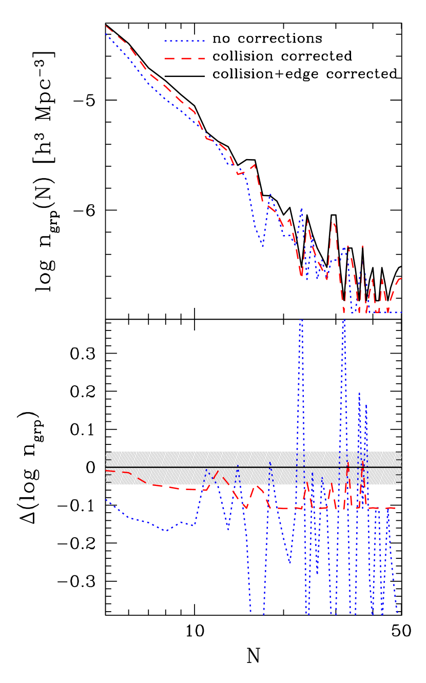
Figure 10.— Differential group multiplicity function for groups identified in the SDSS $Mr20$ volume-limited sample. The different curves are $n_{\mathrm{grp}}(N)$ uncorrected for incompleteness (dotted blue curves), corrected for incompleteness due to fiber collisions (dashed red curves), and corrected for both fiber collisions and edge effects (solid black curves). The bottom panel shows the ratio of each case to the fully corrected one. The shaded region encloses $\pm 10\%$ deviations from the fully corrected multiplicity function. These results are averaged over all of our .Mr20 mock catalogs.

Table 5. Group Multiplicity Function for $Mr20$ Sample

$N_{\mathrm{min}}$–$N_{\mathrm{max}}$	$n_{\mathrm{grp}}(N)$	$\sigma_{n_{\mathrm{grp}}}$	$\sigma_{n_{\mathrm{grp}}}$ (Poisson)
3–3	$2.290\times 10^{-4}$	$1.110\times 10^{-5}$	$5.881\times 10^{-6}$
4–4	$1.054\times 10^{-4}$	$4.890\times 10^{-6}$	$3.990\times 10^{-6}$
5–5	$4.909\times 10^{-5}$	$4.181\times 10^{-6}$	$2.723\times 10^{-6}$
6–6	$3.263\times 10^{-5}$	$4.465\times 10^{-6}$	$2.220\times 10^{-6}$
7–7	$1.962\times 10^{-5}$	$1.979\times 10^{-6}$	$1.722\times 10^{-6}$
8–8	$1.496\times 10^{-5}$	$2.250\times 10^{-6}$	$1.503\times 10^{-6}$
9–9	$1.118\times 10^{-5}$	$2.398\times 10^{-6}$	$1.299\times 10^{-6}$
10–10	$8.906\times 10^{-6}$	$1.502\times 10^{-6}$	$1.160\times 10^{-6}$
11–11	$5.139\times 10^{-6}$	$1.292\times 10^{-6}$	$8.810\times 10^{-7}$
12–12	$4.223\times 10^{-6}$	$8.632\times 10^{-7}$	$7.986\times 10^{-7}$
13–13	$3.780\times 10^{-6}$	$7.200\times 10^{-7}$	$7.555\times 10^{-7}$
14–14	$2.565\times 10^{-6}$	$1.283\times 10^{-6}$	$6.224\times 10^{-7}$
15–15	$2.873\times 10^{-6}$	$9.335\times 10^{-7}$	$6.587\times 10^{-7}$
16–16	$2.868\times 10^{-6}$	$1.165\times 10^{-6}$	$6.581\times 10^{-7}$
17–17	$1.361\times 10^{-6}$	$6.868\times 10^{-7}$	$4.533\times 10^{-7}$
18–18	$1.358\times 10^{-6}$	$4.131\times 10^{-7}$	$4.530\times 10^{-7}$
19–19	$1.209\times 10^{-6}$	$5.133\times 10^{-7}$	$4.273\times 10^{-7}$
20–21	$9.817\times 10^{-7}$	$3.079\times 10^{-7}$	$3.851\times 10^{-7}$
22–24	$6.039\times 10^{-7}$	$2.253\times 10^{-7}$	$3.020\times 10^{-7}$
25–28	$3.401\times 10^{-7}$	$9.522\times 10^{-8}$	$2.266\times 10^{-7}$
29–30	$9.061\times 10^{-7}$	$4.483\times 10^{-7}$	$3.699\times 10^{-7}$
31–34	$3.398\times 10^{-7}$	$7.501\times 10^{-8}$	$2.265\times 10^{-7}$
35–42	$1.699\times 10^{-7}$	$6.455\times 10^{-8}$	$1.602\times 10^{-7}$
43–61	$6.360\times 10^{-8}$	$2.982\times 10^{-8}$	$9.801\times 10^{-8}$

Note—$n_{\mathrm{grp}}$ and $\sigma_{n_{\mathrm{grp}}}$ are in units of $h^{3}{\mathrm{Mpc}}^{-3}$.

We must calculate errorbars for the multiplicity function in order to use it to constrain the HOD. We use our mock catalogs for this purpose. Specifically, we compute fractional errors from the dispersion among 10 independent mock catalogs for the $Mr20$ sample (LANL1-5.Mr20 mocks $\times$ 1 HOD realization $\times$ 2 mocks per simulation cube), and 8 mock catalogs for each of the $Mr19$ and $Mr18$ samples (LANL1-4.Mr19/LANL1-4.Mr18 mocks $\times$ 1 HOD realization $\times$ 2 mocks per simulation cube). Note that we do not use multiple HOD realizations because the underlying halo populations themselves would not be independent. Before computing errors, we correct each mock catalog for fiber collisions and edge effects in the same way as in the data. The computed errors thus implicitly include any contribution from these correction procedures.

The SDSS multiplicity function shown in Figure 10 becomes very noisy at high richness because the abundance of groups drops with $N$ and the figure uses richness bins with a width of unity. It makes more sense to increase the bin width with $N$ so as to beat down the noise. Moreover, since we calculate errorbars for the multiplicity function using our mock catalogs, each richness bin must contain enough mock groups so that an errorbar can be reliably estimated. We choose richness bins for each group catalog so that each bin contains at least eight SDSS groups and twenty mock groups (among all mock catalogs used). At low multiplicities, the bin width is always unity because there are many groups with low $N$. At higher multiplicities, however, the richness bins grow wider in order to satisfy these criteria. The bin widths for samples $Mr20$, $Mr19$, and $Mr18$, are listed in the first columns of Tables 5, 6, and 7, respectively. Once a richness bin is defined, the abundance of groups in that bin, $n_{\mathrm{grp}}(N)$, is simply the number of groups having richnesses within the bin, divided by the sample volume and divided by the bin width. The values of $n_{\mathrm{grp}}(N)$ are listed in the second columns of Tables 5, 6, and 7. We use the same richness bins to compute the abundance of mock groups for each independent mock catalog, and we compute errors, $\sigma_{n_{\mathrm{grp}}}$, in the SDSS multiplicity function by measuring the dispersion among the mock multiplicity functions. These errors are listed in the third columns of Tables 5, 6, and 7. Finally, we also compute Poisson errors for the SDSS $n_{\mathrm{grp}}(N)$, which we list in the fourth columns of Tables 5, 6, and 7. In some of the highest multiplicity bins, the Poisson errors are larger than the mock errors. In these cases, the mock errors are likely underestimated and it is best to use the Poisson errors in their place.

Table 6. Group Multiplicity Function for $Mr19$ Sample

$N_{\mathrm{min}}$–$N_{\mathrm{max}}$	$n_{\mathrm{grp}}(N)$	$\sigma_{n_{\mathrm{grp}}}$	$\sigma_{n_{\mathrm{grp}}}$ (Poisson)
3–3	$4.514\times 10^{-4}$	$2.872\times 10^{-5}$	$1.545\times 10^{-5}$
4–4	$1.889\times 10^{-4}$	$1.201\times 10^{-5}$	$9.996\times 10^{-6}$
5–5	$1.085\times 10^{-4}$	$9.323\times 10^{-6}$	$7.575\times 10^{-6}$
6–6	$6.292\times 10^{-5}$	$8.977\times 10^{-6}$	$5.769\times 10^{-6}$
7–7	$5.027\times 10^{-5}$	$5.465\times 10^{-6}$	$5.157\times 10^{-6}$
8–8	$2.856\times 10^{-5}$	$2.434\times 10^{-6}$	$3.887\times 10^{-6}$
9–9	$1.853\times 10^{-5}$	$2.832\times 10^{-6}$	$3.131\times 10^{-6}$
10–10	$1.534\times 10^{-5}$	$2.799\times 10^{-6}$	$2.849\times 10^{-6}$
11–11	$1.534\times 10^{-5}$	$2.577\times 10^{-6}$	$2.849\times 10^{-6}$
12–12	$1.164\times 10^{-5}$	$2.236\times 10^{-6}$	$2.482\times 10^{-6}$
13–13	$8.994\times 10^{-6}$	$2.135\times 10^{-6}$	$2.181\times 10^{-6}$
14–14	$7.936\times 10^{-6}$	$2.105\times 10^{-6}$	$2.049\times 10^{-6}$
15–15	$5.819\times 10^{-6}$	$1.186\times 10^{-6}$	$1.755\times 10^{-6}$
16–16	$5.819\times 10^{-6}$	$1.718\times 10^{-6}$	$1.755\times 10^{-6}$
17–18	$5.819\times 10^{-6}$	$1.318\times 10^{-6}$	$1.755\times 10^{-6}$
19–20	$2.380\times 10^{-6}$	$5.168\times 10^{-7}$	$1.122\times 10^{-6}$
21–23	$2.292\times 10^{-6}$	$5.243\times 10^{-7}$	$1.101\times 10^{-6}$
24–26	$1.587\times 10^{-6}$	$4.621\times 10^{-7}$	$9.164\times 10^{-7}$
27–32	$7.054\times 10^{-7}$	$2.228\times 10^{-7}$	$6.109\times 10^{-7}$
33–38	$7.054\times 10^{-7}$	$3.069\times 10^{-7}$	$6.109\times 10^{-7}$
39–51	$3.256\times 10^{-7}$	$4.634\times 10^{-8}$	$4.151\times 10^{-7}$
52–86	$1.209\times 10^{-7}$	$3.602\times 10^{-8}$	$2.529\times 10^{-7}$

Note—Same units as Table 5.

Table 7. Group Multiplicity Function for $Mr18$ Sample

$N_{\mathrm{min}}$–$N_{\mathrm{max}}$	$n_{\mathrm{grp}}(N)$	$\sigma_{n_{\mathrm{grp}}}$	$\sigma_{n_{\mathrm{grp}}}$ (Poisson)
3–3	$7.311\times 10^{-4}$	$6.909\times 10^{-5}$	$4.000\times 10^{-5}$
4–4	$3.436\times 10^{-4}$	$3.325\times 10^{-5}$	$2.742\times 10^{-5}$
5–5	$1.948\times 10^{-4}$	$2.200\times 10^{-5}$	$2.065\times 10^{-5}$
6–6	$1.248\times 10^{-4}$	$1.629\times 10^{-5}$	$1.652\times 10^{-5}$
7–7	$1.182\times 10^{-4}$	$1.546\times 10^{-5}$	$1.608\times 10^{-5}$
8–8	$5.686\times 10^{-5}$	$9.917\times 10^{-6}$	$1.116\times 10^{-5}$
9–9	$3.284\times 10^{-5}$	$5.340\times 10^{-6}$	$8.477\times 10^{-6}$
10–10	$3.066\times 10^{-5}$	$5.777\times 10^{-6}$	$8.191\times 10^{-6}$
11–11	$2.626\times 10^{-5}$	$8.403\times 10^{-6}$	$7.581\times 10^{-6}$
12–13	$1.423\times 10^{-5}$	$1.629\times 10^{-6}$	$5.580\times 10^{-6}$
14–15	$8.756\times 10^{-6}$	$1.443\times 10^{-6}$	$4.378\times 10^{-6}$
16–17	$1.203\times 10^{-5}$	$1.761\times 10^{-6}$	$5.132\times 10^{-6}$
18–23	$3.647\times 10^{-6}$	$7.402\times 10^{-7}$	$2.825\times 10^{-6}$
24–31	$2.188\times 10^{-6}$	$6.091\times 10^{-7}$	$2.188\times 10^{-6}$
32–152	$1.447\times 10^{-7}$	$1.673\times 10^{-8}$	$5.627\times 10^{-7}$

Note—Same units as Table 5.

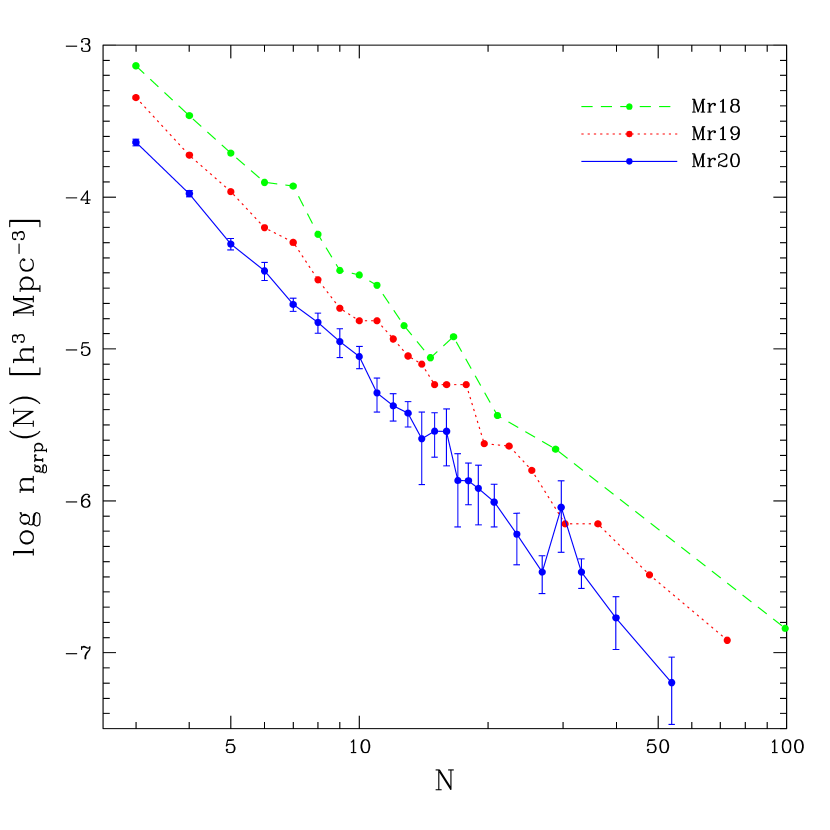
Figure 11.— Differential group multiplicity functions for SDSS groups. The three curves show $n_{\mathrm{grp}}(N)$ for groups identified in our three volume-limited samples: $Mr20$, $Mr19$, and $Mr18$ (colors and line types are listed in the top-right corner of the panel). $n_{\mathrm{grp}}(N)$ is measured in richness bins whose widths are chosen so that the bins contain a minimum of 8 SDSS groups and 20 mock groups. Points are placed at the mean richness of groups within each bin. Errors are shown for the $Mr20$ sample and are estimated from the dispersion among 10 independent SDSS mock catalogs.

Figure 11 shows the SDSS multiplicity functions for the three volume-limited samples, along with the mock errorbars for the $Mr20$ sample. Though we measure and show the multiplicity function down to a multiplicity of $N=3$, our tests with mock catalogs have shown that it is only unbiased with respect to the true halo multiplicity function for $N\geq 10$. When using this measured multiplicity function to constrain the HOD, we must either only use bins with $N\geq 10$, or attempt to calibrate the relation between the measured group multiplicity function and the true halo multiplicity function at lower values of $N$. The central curve of Figure 14, discussed in the Appendix, effectively provides this calibration for $Mr20$ and the cosmology adopted in our mock catalogs.

The multiplicity functions shown in Figure 11 appear to be close to power-law relations. In order to test this, we perform a simple power-law fit to each multiplicity function in the regime $N\geq 10$. We use only the diagonal errors of the full covariance matrix (i.e., the errors listed in Tables 5, 6, and  7). We find that all three multiplicity functions are well-fit by power-law relations, with best-fit slopes of $-2.72\pm 0.16$, $-2.48\pm 0.14$, and $-2.49\pm 0.28$ for the $Mr20$, $Mr19$, and $Mr18$ samples, respectively.

8. Summary and Discussion

We have used a simple friends-of-friends algorithm to identify galaxy groups in volume-limited samples of the SDSS redshift survey. We have selected FoF linking lengths that are best at grouping together galaxies that occupy the same dark matter halos. We based this choice on extensive tests with mock galaxy catalogs, which we constructed by populating halos in N-body simulations with galaxies. The result of our mock tests is that no combination of perpendicular and line-of-sight linking lengths can yield groups that successfully recover all aspects of the parent halo distribution, even for large richness systems. Specifically, FoF cannot identify groups that simultaneously have unbiased abundances, projected sizes, and velocity dispersions. The ideal group-finding parameters for a given study depend on its scientific objectives. Given our objective of using the multiplicity function to constrain the HOD, it makes sense to sacrifice velocity dispersions and obtain groups with unbiased abundances and projected sizes. Our choice of linking lengths results in a group catalog that, for groups of ten or more members, has an unbiased multiplicity function, an unbiased median relation between the multiplicities of groups and their parent halos, an unbiased projected size distribution as a function of multiplicity, and a velocity dispersion distribution that is $\sim 20\%$ too low for all multiplicities. We correct for fiber collisions and survey edge effects and present three SDSS group catalogs (for three different volume-limited samples) and their measured multiplicity functions.

It is important to recognize that our adopted group finder has the above properties only for halos defined using FoF with a linking length of 0.2 times the mean interparticle separation, since this is how halos were identified in our mock catalogs. A different halo definition (such as FoF with a different linking length, or spherical overdensity halos) would require a different set of optimal group-finding parameters. This is not a problem as long as the same halo definition is used consistently. For example, an HOD measured from these group catalogs will hold for this halo definition, and any theoretical model should use the same halo definition to compare its predictions to the measured HOD. We chose this particular halo finder because it has been widely used and tested, and the properties of the resulting halo distribution (e.g., mass function) are well understood.

The groups and clusters that we present here are intended to be systems of galaxies that belong to the same virialized dark matter halo. We can test whether these systems are virialized by computing crossing times for the groups and checking if they are sufficiently less than the Hubble time. We define the crossing time divided by the hubble time as

$$\frac{t_{\mathrm{cross}}}{t_{\mathrm{H}}}=\frac{(R_{\mathrm{rms}}/h^{-1}\mathrm{Mpc})}{(\sigma_{v}/100{\,{\rm km}\,{\rm s}^{-1}})},$$ (9)

where $R_{\mathrm{rms}}$ is the one-dimensional group radius, which is equal to the projected (two-dimensional) radius, $R_{\perp,\mathrm{rms}}$, divided by the square root of two. We correct for the velocity dispersion bias revealed in our mock tests by applying a 20% upward correction to all group velocity dispersions, and we compute $t_{\mathrm{cross}}/t_{\mathrm{H}}$ for all groups. We find that, for all three group catalogs, the median value of $t_{\mathrm{cross}}/t_{\mathrm{H}}$ is $\sim 0.15$, and 80% of all groups have values less than $\sim 0.29$. These numbers can be interpreted in terms of the spherical infall model (gunn_gott_72; gott_turner_77a), or other analytic or numerical models. However, at a first glance, the numbers are encouraging and suggest that most of our groups are likely virialized systems.

The group and cluster catalogs presented here are well-suited for testing many of the predictions and assumptions made by galaxy formation models regarding the relationship between galaxies and their underlying dark matter halos. We will investigate several of these issues in subsequent papers.

Appendix

In this appendix, we describe the mock catalog tests that help us choose optimal FoF parameters. Since our primary goal for identifying groups is to measure the group multiplicity function and use it to constrain the HOD, we clearly require our FoF algorithm to produce groups that have an unbiased multiplicity function with respect to the true halo multiplicity function. In addition, we require an unbiased relation between the multiplicities of groups and their associated halos. Finally, we would like our groups to have unbiased projected size and velocity dispersion distributions as a function of multiplicity. We create a grid of FoF linking lengths and check how each set of linking lengths performs in the above tests, for each of the four HOD model mock cubes (.Mr20, .Mr20b, .Mr19, .Mr18). In the case of each HOD model, we average results over the 10 HOD realizations described in § 3 and over the LANL1 and LANL4 N-body simulations.

Before focusing on redshift space, we briefly examine how well FoF recovers the true multiplicity function in real space, since this represents the best possible case (any group finder will almost certainly perform worse in redshift space). We apply FoF to the real-space cube mocks using a single linking length (the linking volume around each mock galaxy is a sphere), and investigate how the recovered multiplicity function varies with the value of this linking length. In particular, we compare the mock group multiplicity functions to the input halo multiplicity functions that were used to construct the mock catalogs. Figure 12 shows this comparison for the .Mr20 mocks. The bottom panel of the figure shows the logarithm of the ratio of group to halo multiplicity function, and the horizontal solid line therefore denotes the “unbiased” case. The figure reveals that, at large $N$, the group multiplicity function has an unbiased shape that is independent of the choice of linking length (at least for the range of linking lengths shown). The amplitude, however, is dependent on the linking length used, with larger linking lengths leading to a higher abundance of groups at large $N$. A linking length of $b=0.2$ (in units of the mean intergalaxy separation) yields a group multiplicity function with an unbiased amplitude at large $N$. This is not surprising given that the same value was used to identify dark matter halos in the N-body simulations while constructing mock catalogs.

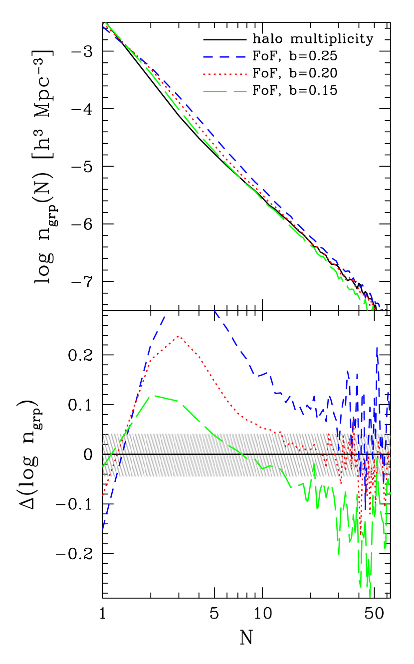
Figure 12.— Effect of changing the FoF linking length on the group multiplicity function in real space, measured using mock galaxy catalogs (described in § 3). In the top panel, the solid black curve shows the input halo multiplicity function for mock catalogs and thus represents the “true” case. The other three curves show the recovered group multiplicity functions for three different linking lengths, which are listed at the top right of the panel in units of the mean inter-galaxy separation. The bottom panel shows the ratio of each case to the “true” one. The shaded region encloses $\pm 10\%$ deviations from the “true” multiplicity function. These results are averaged over all of our .Mr20 mock catalogs.

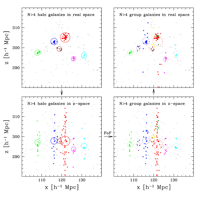
Figure 13.— Illustrated behavior of the Friends-of-Friends (FoF) group finder. Each panel shows a $40\times 40\times 10h^{-1}\mathrm{Mpc}$ slice through a mock galaxy catalog. Moving counter-clockwise starting from the top left panel, the panels show: galaxies in dark matter halos in real space (top left), the same galaxies in redshift space (bottom left), galaxies in groups recovered using FoF (bottom right), and these group galaxies in their real-space positions (top right). In each case, galaxies in halos or groups with $N>4$ are shown as colored points, with each halo or group represented by a unique color. Large open circles are centered on the halo or group centers and have radii equal to the halo virial radii (left panels) and the estimated group virial radii (right panels).

At low $N$, the multiplicity function is highly biased, both in shape and amplitude. The abundance of groups relative to halos at a given multiplicity $N$ decreases when FoF splits these halos into smaller groups or merges them to form larger groups. This decrease is countered by an increase due to the merging of smaller halos or the splitting of larger halos. The balance between these competing effects determines whether the multiplicity function is biased or not. For linking lengths near $b=0.2$, merging dominates over splitting, which means that group abundances at a given multiplicity are mainly determined by a balance between halos at that $N$ merging to yield larger groups and smaller halos merging to replenish the lost groups. However, this balance breaks at $N=1$ because, while FoF merges $N=1$ halos (i.e., isolated galaxies) to form larger groups, there are no smaller halos that can merge to replenish $N=1$ groups. The abundance of $N=1$ groups is therefore necessarily less than that of $N=1$ halos (it can only be more if the linking length is so small - approximately $b\sim 0.1$ - that single galaxy groups splinter off in large numbers from larger halos). Since most galaxies live in $N=1$ halos ($\sim 70\%$ in these mock catalogs), merging a small fraction of them to form larger groups will fractionally increase the abundance of larger $N=2,3,4$, etc. groups significantly. This is seen in Figure 12: the abundance of $N=1$ groups is lower than that of halos by $\sim 20\%$ for $b=0.2$, causing the abundance of $N=2$ and $N=3$ groups to be $\sim 50\%$ higher. Only for $N>10$ does the group abundance settle down and become unbiased. This behavior is a fundamental limitation of the FoF algorithm, and it has the consequence that group abundances can only be trusted for large multiplicity groups.

In redshift space, group finding is much more challenging because finger-of-god distortions stretch groups along the line-of-sight, making it more likely that single halos will be split into multiple groups and that neighboring halos will be merged into the same groups. Figure 13 illustrates these effects by showing the performance of FoF in a small slice through a single mock catalog (one HOD realization of the LANL4.Mr20 mock catalog). The top-left panel shows the mock galaxies in real space, with each $N>4$ halo denoted by a unique color. The bottom-left panel shows the same galaxies in redshift space, where the line-of-sight is oriented along the $z$-axis of the mock cube. Large open circles have radii equal to the halo virial radii and are centered at the halo centers in real space, and the galaxy centroids in redshift space. We run our adopted FoF group-finder (described in § 4) on the redshift-space mock and denote each resulting $N>4$ group with a unique color in the bottom-right panel. Finally, we show the group galaxies’ real-space positions in the top-right panel. Large dotted circles are centered at the group centroids and have virial radii that are estimated by assuming a halo mass function and a monotonic relation between group multiplicity and mass. A visual comparison of the real- and redshift-space panels reveals many of the failure modes of FoF group-finding in redshift space. The halo denoted by green in the left-side panels is fairly well recovered by FoF as the group denoted by green in the right-side panels. However, a couple of halo galaxies are missed in group finding, such as the one whose velocity moved it the furthest away from the center of the halo. Most of the galaxies in the halo denoted by blue are linked together in the same group, also denoted by blue. However, many galaxies that do not belong to the “blue” halo are also linked to the same group. This is seen clearly in the top-right panel, where seven of the “blue” group galaxies’ real-space positions place them well outside the halo. A similar thing occurs to the halos and corresponding groups denoted by magenta and cyan. Most of the galaxies in the large “red” halo are recovered correctly into the “red” group, but there are some galaxies added to this group that do not belong to the “red” halo, as well as a few galaxies that do belong to that halo, but have splintered off into a different group (denoted by dark green). Despite these imperfections, there is clearly a substantial correspondence between the groups identified by FoF and the true population of halos in this slice.

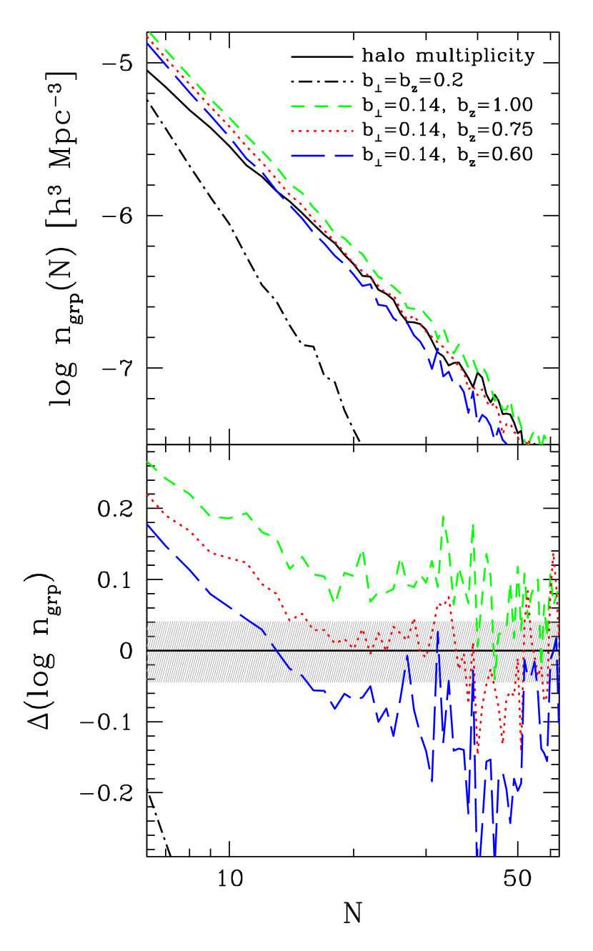
Figure 14.— Same as Fig. 12, but for redshift space. The solid black curve shows the input halo multiplicity function. The dot-dashed black curve shows the recovered group multiplicity function if a single linking length is used. The other three curves show the recovered multiplicity functions for fixed perpendicular and three different line-of-sight linking lengths, which are listed in the top panel in units of the mean inter-galaxy separation. All other features are as in Fig. 12.

We now examine the relative multiplicity functions of groups and halos when the groups are identified in redshift space. If we use the same linking length in transverse and line-of-sight directions, finger-of-god distortions will cause halos to be split into multiple small groups along the line-of-sight. This is demonstrated by the dashed curve in Figure 14, which shows the multiplicity function of groups identified with a single linking length of $b=0.2$. The abundance of groups is vastly underestimated for $N\gtrsim 5$, and the effect grows with $N$ because richer halos have higher velocity dispersions. We therefore need to use different linking lengths in the line-of-sight and perpendicular directions. We apply FoF to our redshift-space cube mocks for a grid of perpendicular and line-of-sight linking lengths and find that we can recover an unbiased multiplicity function at large $N$ for the right combinations of linking lengths. Figure 14 shows one such combination ($b_{\perp}=0.14$, $b_{z}=0.75$) and demonstrates how the group multiplicity function changes with the line-of-sight linking length $b_{z}$. Generally, larger linking lengths in either direction lead to a higher abundance of groups at large $N$. We record all linking length combinations that yield unbiased multiplicity functions in the large $N$ regime and show the successful parameter space in Figure 3, as discussed in § 4.

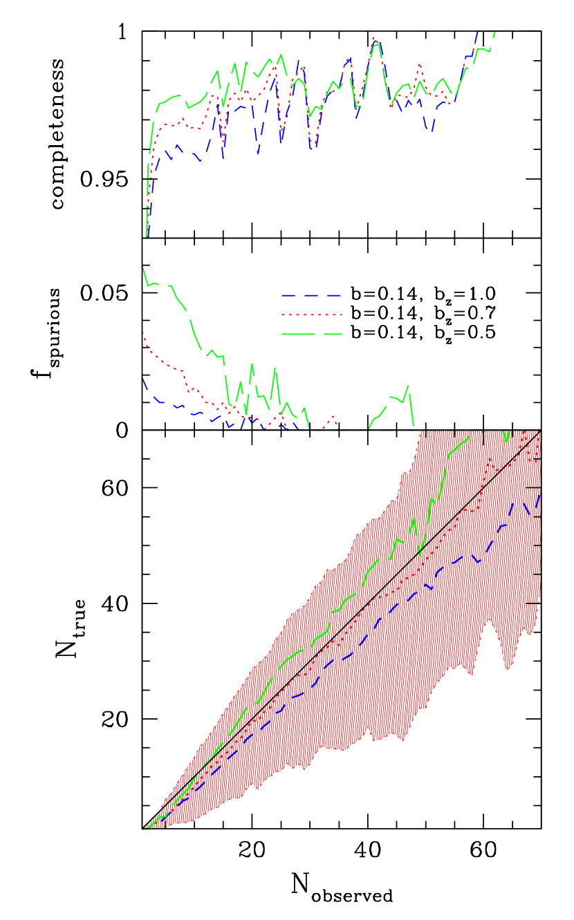
Figure 15.— Effect of changing the FoF linking lengths on the relation between the distributions of input halo richness and recovered group richness in redshift space, measured using mock galaxy catalogs. Each input halo is matched one-to-one to a recovered group whenever possible; however, some halos have no corresponding group and some groups have no one-to-one parent halo. The top panel shows the halo completeness as a function of halo richness, i.e., the fraction of halos at each richness that can be matched one-to-one with a recovered group. The middle panel shows the spurious fraction of groups as a function of group richness, i.e., the fraction of groups at each richness that cannot be matched one-to-one with a parent halo. The bottom panel shows the relation between halo and group richness for halos and groups that are matched one-to-one. Middle curves show the median relation and outer curves show the 10 and 90 percentiles (they enclose $80\%$ of the group-halo pairs). The area between these outer curves is shaded. In all panels, different line types and colors show fixed perpendicular and different line-of-sight linking lengths, which are listed in the top panel in units of the mean inter-galaxy separation. To avoid confusion, the 10 and 90 percentile curves (as well as the shading between them) in the bottom panel are only shown for one of the linking length combinations. All results are averaged over twenty mock galaxy catalogs.

Recovering an unbiased multiplicity function does not guarantee that the one-to-one relation between the multiplicities of halos and their recovered groups is also unbiased. We therefore also investigate this relation. As described in § 4, we associate each halo to the recovered group that contains the halo’s central galaxy. Groups that contain central galaxies from more than one halo are associated with the halo with which they share the largest number of galaxies. Halos that end up not being associated with any group are considered “undetected,” and groups that are not associated with any halo (i.e., they contain no halo central galaxies) are considered “spurious”. Once we have associated mock groups one-to-one with their parent halos, we can look at the relation between the halo and group multiplicities (i.e., $N_{\mathrm{true}}$ vs. $N_{\mathrm{obs}}$). In addition, we can look at the fraction of halos that are detected and the fraction of groups that are spurious. Figure 15 shows how these relations depend on the line-of-sight linking length. The bottom panel of the figure shows one set of linking lengths ($b_{\perp}=0.14$, $b_{z}=0.70$) that yields an unbiased median relation between $N_{\mathrm{true}}$ and $N_{\mathrm{obs}}$, but the scatter around this relation is large and quite asymmetric. 90% of groups at a given $N_{\mathrm{obs}}$ are associated with halos that have up to 40% higher and 60% lower $N_{\mathrm{true}}$. Increasing the line-of-sight linking length causes groups to grow and thus biases the median $N_{\mathrm{true}}$ vs. $N_{\mathrm{obs}}$ relation by tilting it toward larger $N_{\mathrm{obs}}$. As before, we record all linking length combinations that yield unbiased median relations between group and halo multiplicities, and we show the successful parameter space in Figure 3.

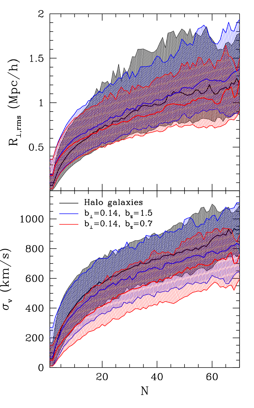
Figure 16.— Effect of changing the FoF linking lengths on the size distribution of groups in redshift space, measured using mock galaxy catalogs. The top panel shows the projected 2-dimensional rms group radius distribution as a function of group richness $N$. The bottom panel shows the same for the 1-dimensional line-of-sight velocity dispersion $\sigma_{v}$. In both panels, the black curves and shading show the size distributions of galaxy systems that occupy the same dark matter halo and thus represent the “true” cases. The sets of colored curves and shadings show the size distributions of recovered groups for fixed perpendicular and three different line-of-sight linking lengths, which are listed in the bottom panel in units of the mean inter-galaxy separation. Middle curves show the median relation and outer curves show the 10 and 90 percentiles. The area between these outer curves is shaded. All results are averaged over twenty mock galaxy catalogs.

The top panel of Figure 15 shows the completeness (fraction of halos that are associated one-to-one with groups) as a function of halo multiplicity $N_{\mathrm{true}}$, and the middle panel shows the spurious group fraction as a function of group multiplicity $N_{\mathrm{obs}}$. Over a wide range of FoF linking lengths, the completeness for halos with $N\gtrsim 5$ is over 95%, and the spurious fraction for groups with $N\gtrsim 5$ is less than 5%. Increasing the line-of-sight linking length causes a drop in the halo completeness and a corresponding drop in the spurious group fraction, since more halos get linked to the same groups. For the final linking lengths that we use (see § 4), the halo completeness is greater than 97% and the spurious group fraction less than 1% for $N\gtrsim 10$. The high completeness and low spurious fraction are a result of how we associate groups to halos. Since we only require a group to have a halo’s central galaxy in order to be associated with it, most groups and halos have one-to-one associations. If we used a more stringent criterion for group-halo association, for example by requiring that a group contain some minimum fraction of a halo’s galaxies, then the halo completeness would be lower and the spurious group fraction higher, but the scatter in $N_{\mathrm{true}}$ vs. $N_{\mathrm{obs}}$ would be reduced. The three panels of Figure 15, put together, characterize the errors in the FoF group finder. Changing the definition for how groups are associated to halos does not change the errors in group-finding; it merely redistributes the errors among the three panels.

In addition to requiring that our groups have unbiased abundances and multiplicities, we would also like them to have unbiased size distributions. For every group in our redshift-space cube mocks, we measure the projected rms radius and the line-of-sight velocity dispersion of galaxies. We compare these to the projected rms radii and actual velocity dispersions of halo galaxies. Figure 16 shows the median, 10th, and 90th percentile projected size and velocity dispersion as a function of multiplicity for halos, compared to that for groups identified with two different line-of-sight linking lengths. Increasing the line-of-sight linking length produces groups with higher velocity dispersions, but it has less impact on the projected size distributions. The opposite is naturally true when we increase the perpendicular linking length. Linking length combinations that yield groups with unbiased abundances and projected sizes tend to yield velocity dispersions that are biased low. This is illustrated in Figure 16, which shows that the linking length combination $b_{\perp}=0.14$, $b_{z}=0.7$ yields groups with velocity dispersions that are $\sim 20\%$ too low relative to halos. The line-of-sight linking length must be more than doubled to repair this bias, but then the abundances of groups would be too high.

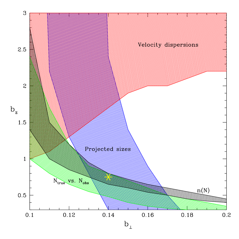
Figure 17.— Same as Fig. 3, but using the .Mr20b set of mock catalogs, which are constructed with a different input relation between halo richness and dark matter halo mass, as described in § 3.

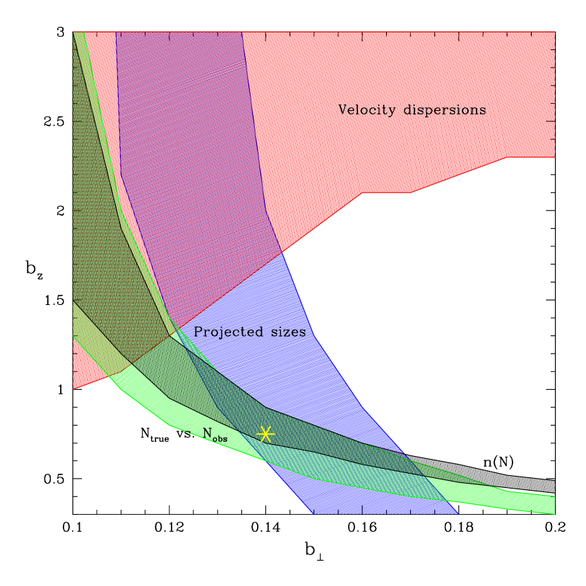
Figure 18.— Same as Fig. 3, but using the .Mr19 set of mock catalogs, described in § 3.

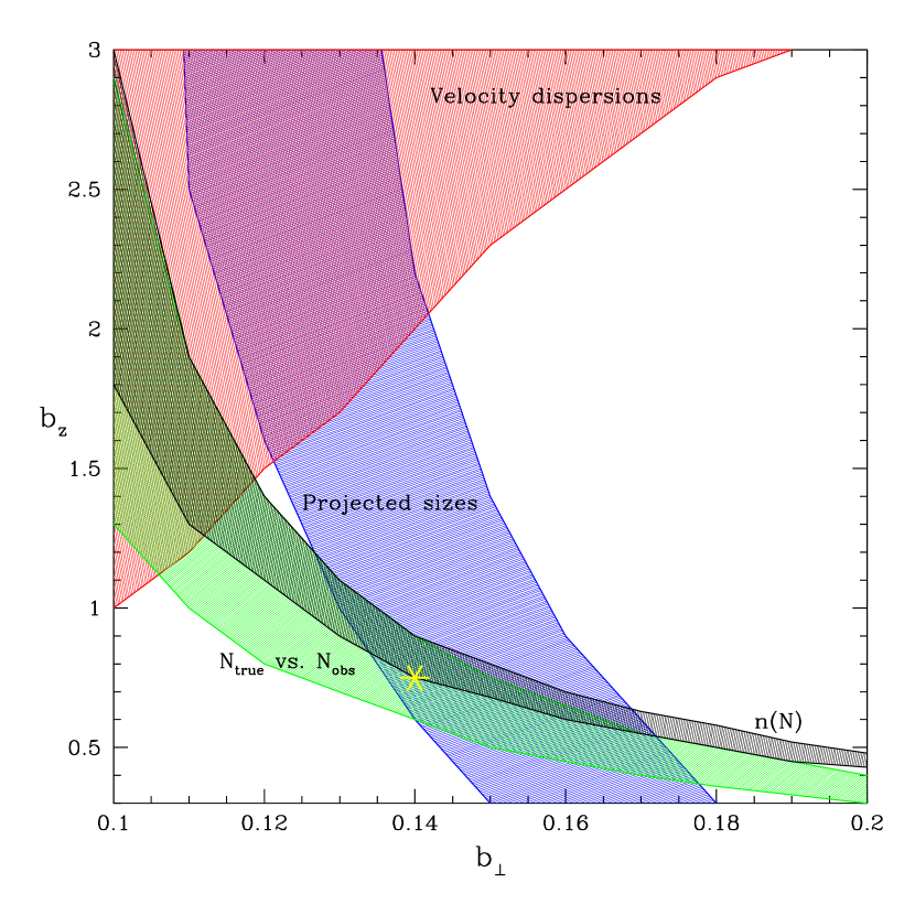
Figure 19.— Same as Fig. 3, but using the .Mr18 set of mock catalogs, described in § 3.

Figure 3 shows the linking length parameter space that satisfies each of the above tests. As discussed in § 4, there is no combination of perpendicular and line-of-sight linking lengths that yields groups with unbiased abundances, projected sizes, and velocity dispersions, even at high multiplicity. We choose to sacrifice velocity dispersions and adopt the parameters $b_{\perp}=0.14$, $b_{z}=0.75$. All the above tests and resulting choice of linking lengths were done using the .Mr20 mock catalogs. Since we plan to use our group catalog to constrain the HOD, it is vital that our choice of linking lengths does not depend sensitively on the input HOD assumed when constructing the mocks. For this reason, we repeat all the above tests with the .Mr20b mock catalogs, which use a different input HOD to model the same $Mr20$ sample of SDSS galaxies. The results are shown in Figure 17. It is clear that our adopted group finder performs equally well in both sets of mock catalogs, demonstrating that our choice of linking lengths is insensitive to the underlying HOD. It is also important to show how well our linking lengths work on lower luminosity galaxy samples, since we apply them to the SDSS $Mr19$ and $Mr18$ samples. We thus repeat our mock tests with the .Mr19 and .Mr18 mock catalogs and show the results in Figures 18 and 19, respectively. The figures show that lower luminosity (higher density) samples require slightly higher line-of-sight linking lengths in order to retain unbiased multiplicity functions. However, this effect is small. When applied to the .Mr18 mock catalogs, our adopted linking lengths yield a multiplicity function that is 10% too low in amplitude. Overall, Figures 3, 17, 18, and 19 demonstrate that our choice of linking lengths is fairly robust.