astro-ph/0601333

January 2006

Constraints on the coupled quintessence from cosmic microwave background anisotropy and matter power spectrum

Seokcheon Lee¹, Guo-Chin Liu,² and Kin-Wang Ng^1,2

¹Institute of Physics,
Academia Sinica, Taipei, Taiwan 11529, R.O.C.

²Institute of Astronomy and Astrophysics,
Academia Sinica, Taipei, Taiwan 11529, R.O.C.

Abstract

We discuss the evolution of linear perturbations in a quintessence model in which the scalar field is non-minimally coupled to cold dark matter. We consider the effects of this coupling on both cosmic microwave background temperature anisotropies and matter perturbations. Due to the modification of the scale of cold dark matter as $\rho_{c}=\rho_{c}^{(0)}a^{-3+\xi}$, we can shift the turnover in the matter power spectrum even without changing the present energy densities of matter and radiation. This can be used to constrain the strength of the coupling. We find that the phenomenology of this model is consistent with current observations up to the coupling power $n_{c}\leq 0.01$ while adopting the current parameters measured by WMAP. Upcoming cosmic microwave background observations continuing to focus on resolving the higher peaks may put strong constraints on the strength of the coupling.

1 Introduction

Analysis of the Hubble diagram of high redshift Type Ia supernovae (SNe Ia) has discovered that the expansion of the Universe is currently accelerating [1]. In addition, combining measurements of the acoustic peaks in the angular power spectrum of the cosmic microwave background (CMB) anisotropy which indicate the flatness of the Universe [2] and the matter power spectrum of large scale structure (LSS) which is inferred from galaxy redshift surveys like the Sloan Digital Sky Survey (SDSS) [3] and the $2$-degree Field Galaxy Redshift Survey ($2$dFGRS) [4] has confirmed that a component with negative pressure (dark energy) should be added to the matter component to make up the critical density today.

The cosmological constant and/or a quintessence field are the most commonly accepted candidates for dark energy. The latter is a dynamical scalar field leading to a time dependent equation of state, $\omega_{\phi}$. Also, this scalar field has a fluctuating, inhomogeneous component in order to conserve the equivalence principle corresponding to the response of the new component to the inhomogeneities in the surrounding cosmological fluid [5].

Several new observational effects produced by the existence of quintessence are imprinted in the CMB anisotropies and the matter power spectrum when compared to models with the cosmological constant. The locations of the acoustic peaks in the CMB angular power spectrum are shifted due to their dependence on the amount of dark energy today and at last scattering as well as $\omega_{\phi}$ [6, 7]. Usually the Universe is dominated by the quintessence at late times ($z\sim{\cal O}(1)$), when the gravitational potential associated with the density perturbations is changed due to a time dependent $\omega_{\phi}$. This enhances the CMB anisotropies at large angular scales by the integrated Sachs-Wolfe effect (ISW) [8]. Thus the amplitudes of both CMB angular and matter power spectra decrease at large scale for the fixed Cosmic Background Explorer Satellite (COBE) normalization compared to those in the cold dark matter model with a cosmological constant ($\Lambda$CDM) [9].

The possibility that a scalar field at early cosmological times follows an attractor-type solution and tracks the evolution of the visible matter-energy density has been explored [10]. This may help alleviate the severe fine-tuning associated with the cosmological constant problem. However, this still cannot explain the reason why the dark energy and the dark matter have comparable energy densities at present. Recently models considering the coupling of quintessence to dark matter have been investigated as a possible solution for this late time coincidence problem [11]. However, several of these models using a simple coupling can be ruled out by observational constraints [12].

These non-minimally coupled quintessence models have several different observational effects compared to the minimally coupled models. One of the most important effects is a different scaling of the cold dark matter (CDM) compared to that of CDM of the minimally coupled case. Since CDM scales as $\rho_{c}=\rho_{c}^{(0)}a^{-3+\xi}$ where $\xi<0$, there will be more CDM energy density at early epoch compared to the case with $\xi=0$ (i.e. $n_{c}=0$). As the coupling is increased, the locations of the acoustic peaks are also shifted to smaller scales. However, the amplitudes of the odd-number peaks decrease due to the decrease of the baryon density at early time and the increasing ISW effect as the coupling scaled with the COBE normalization. The amplitudes of the even-number peaks increase due to the increase of the CDM energy density. Even though the ratios of the height of the first peak to those of higher peaks between different couplings are quite similar to one another, these are quite different from the $\Lambda$CDM model [13]. The location of the turnover in the matter power spectrum corresponds to the scale that entered the Hubble radius when the universe became matter-dominated ($a_{eq}$). Thus the coupling might shift the turnover scale.

This paper is organized as follows. In the next section we show the basic equations of linear perturbations of the coupled quintessence model. In Sec. 3, we derive the formal entropy perturbation due to multiple fluids. We also consider the possibility of isocurvature perturbations of the quintessence. We check the coupling effects on CMB and matter power spectrum in Sec. 4. The effect of coupling on the metric perturbation is considered in Sec. 5. Our conclusion is in the last section.

2 Linear perturbations

We will consider the perturbation effect of the quintessence model which is coupled to the CDM. First we start from the metric in the conformal Newtonian (longitudinal) gauge, which is restricted only for the scalar mode of the metric perturbations [14]. The line element is given by

$$ds^{2}=a^{2}(\eta)\Biggl{[}-\Bigl{(}1+2\Psi(\eta,\vec{x})\Bigr{)}d\eta^{2}+\Bigl{(}1-2\Phi(\eta,\vec{x})\Bigr{)}dx^{i}dx_{i}\Biggr{]},$$ (2.1)

where $\eta$ is the conformal time, $\Psi$ is the amplitude of perturbation in the lapse function, and $\Phi$ is the amplitude of perturbation of a unit spatial volume. We will consider only a flat universe case. If the coupling is derived by a Brans-Dicke Lagrangian, the radiation is decoupled from the dark energy [15]. Due to the strong constraint on the coupling to the baryons from the local gravity experiments such as radar time-delay measurements, we will assume that the baryons are decoupled from quintessence [16]. Also from the violation of the weak equivalence principle, even though it is in a still way that is locally unobservable, we can have the species-dependent couplings [17]. So we will make an assumption that the scalar field $\phi$ is coupled only to CDM by means of a general function $\exp[B_{c}(\phi)]$ and there is no coupling to the baryons or the radiation [18]. We can write the general equation including this interaction as

$$S=-\int d^{4}x\sqrt{-g}\Biggl{\{}\frac{\bar{M}^{2}}{2}[\partial^{\mu}\phi\partial_{\mu}\phi-R]+V(\phi)-{\cal L}_{c}-{\cal L}_{r}-{\cal L}_{b}\Biggr{\}},$$ (2.2)

where $\bar{M}=1/\sqrt{8\pi G}$ is the reduced Planck mass and ${\cal L}_{i}$s denote respectively CDM, radiation, and baryons. If we regard the matter as a gas of pointlike particles with masses $m_{c}$ and paths $x_{c}^{\nu}(t)$, then we can write ${\cal L}_{c}$ as

$${\cal L}_{c}=-\frac{m_{c}}{\sqrt{-g}}\delta(\vec{x}-\vec{x}_{c}(t))(-g_{\mu\nu}\dot{x}_{c}^{\mu}\dot{x}_{c}^{\nu})^{1/2},$$ (2.3)

where $m_{c}=e^{B_{c}(\phi)}m^{*}_{c}$ ($m_{c}^{*}$ being a bare mass of the CDM)  [19, 20]. Each fluid element has an energy-momentum tensor $T^{\mu}_{(\beta)\nu}$ where $\beta$ includes all of the species. The total energy-momentum tensor is covariantly conserved, however the energy-momentum transfer between CDM and quintessence is written as

$$\sum_{\beta}\nabla_{\mu}T^{\mu}_{(\beta)\nu} = 0,$$ (2.4)

$$\nabla_{\mu}T^{\mu}_{(\gamma)\nu} = 0,$$ (2.5)

$$\nabla_{\mu}T^{\mu}_{(d)\nu} = Q_{(d)\nu},$$ (2.6)

where $\gamma$ denotes baryons or radiation, $d$ denotes CDM or quintessence, and $Q_{(d)\nu}$ is the energy-momentum transfer vector which shows the energy transfer to the $d$-fluid [21]. This transfer vector is constrained as

$$\sum_{d}Q_{(d)\nu}=0.$$ (2.7)

From the above action (2.2) we have the following equation which will give the constraint equation for the interaction between the quintessence and the CDM:

$$\bar{M}^{2}\Box\phi-\frac{\partial V}{\partial\phi}-\frac{\partial B_{c}}{\partial\phi}{\cal L}_{c}=0.$$ (2.8)

From this we can find the unperturbed part of the field equation,

$$\phi^{\prime\prime}+2{\cal H}\phi^{\prime}+\frac{a^{2}}{\bar{M}^{2}}\frac{\partial V(\phi)}{\partial\phi}=-\frac{a^{2}}{\bar{M}^{2}}\frac{\partial B_{c}(\phi)}{\partial\phi}\rho_{c},$$ (2.9)

where the prime means $d/d\eta$, ${\cal H}=a^{\prime}/a$, and $\rho_{c}$ means the energy density of CDM. As we mentioned before the energy-momentum of each species may not be conserved due to the scalar field coupling even though the total energy momentum does conserve. If we use this fact, then we can rewrite Eqs. (2.4), (2.5), and (2.6) as

$$\rho_{\rm{tot}}^{\prime} = -3{\cal H}(\rho_{\rm{tot}}+p_{\rm{tot}}),$$ (2.10)

$$\rho_{\gamma}^{\prime} = -3{\cal H}(\rho_{\gamma}+p_{\gamma}),$$ (2.11)

$$\rho_{c}^{\prime} = -3{\cal H}(\rho_{c}+p_{c})+B_{c,\phi}\phi^{\prime}\rho_{c}\equiv-3{\cal H}(\rho_{c}+p_{c})(1-{\cal B}_{c}),$$ (2.12)

$$\rho_{\phi}^{\prime} = -3{\cal H}(\rho_{\phi}+p_{\phi})-B_{c,\phi}\phi^{\prime}\rho_{c}\equiv-3{\cal H}(\rho_{\phi}+p_{\phi})(1-{\cal B}_{\phi}),$$ (2.13)

where $B_{c,\phi}=\partial B_{c}/\partial\phi$. Henceafter we will adopt the potential and the coupling as given in Ref. [20]:

$$V(\phi) = V_{0}\exp\Bigl{(}\frac{\lambda\phi^{2}}{2}\Bigr{)},$$ (2.14)

$$\exp[B_{c}(\phi)] = \Biggl{(}\frac{b_{c}+V(\phi)/V_{0}}{1+b_{c}}\Biggr{)}^{n_{c}},~{}~{}~{}{\rm with}~{}~{}b_{c}+1>0,$$ (2.15)

where $V_{0}$, $\lambda$, $b_{c}$, and $n_{c}$ are constant parameters. Here we will consider only $b_{c}=0$ case.

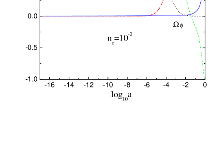
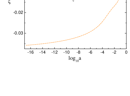
Figure 1: (a) Cosmological evolution of the equation of state parameter, $\omega_{\phi}$, and the energy density parameters, $\Omega_{i}$, of each component for $\lambda=5$ and $n_{c}=10^{-2}$. The evolution of the parameters is similar for other choices of $\lambda$. (b) Deviations of the scaling of the CDM energy density ($\xi$) from $a^{-3}$ for couplings with $n_{c}=10^{-3}$ (dashed line) and $n_{c}=10^{-2}$ (dash-dotted line).

From these we have the evolution of the background quantities as shown in the first panel of Fig. 1. The parameters we use in this figure for the present energy density contrasts of the quintessence and the CDM are $\Omega_{\phi}^{(0)}=0.76$ and $\Omega_{c}^{(0)}=0.20$, respectively. To be compatible with observational data, the energy density of the quintessence must be subdominant during the big-bang nucleosynthesis (BBN) $\Omega_{\phi}^{\rm{BBN}}(a\sim 10^{-10})<0.2$ at $T\sim 1\,{\rm MeV}$ [10], and the energy density at present must be comparable to the preferred range for dark energy, $0.60\leq\Omega_{\phi}^{(0)}(a=0)\leq 0.85$  [2]. The stronger bound on the energy density of the quintessence during BBN, $\Omega_{\phi}^{\rm{BBN}}(a\sim 10^{-10})<0.045$ [22], is also well satisfied in this model. We note that the equation of state (EOS) of the quintessence $\omega_{\phi}\equiv p_{\phi}/\rho_{\phi}\approx\omega_{r}=1/3$ during the radiation dominated era as in other tracker solutions. Instead of falling from the tracking value of $1/3$ towards $-1$, as in the uncoupled case, $\omega_{\phi}$ increases towards higher values ($\leq+1$), before ultimately dropping to $-1$ at later times. This is due to the fact that when the matter density increases, the effect on the effective potential $V_{eff}(\phi)=V(\phi)+\rho_{c}$ given in Eq. (2.9) drives the faster evolution of $\phi$. From Eq. (2.12), we find that the scaling of the CDM energy density differs from the usual $a^{-3}$ due to the coupling :

$$\rho_{c}(a) = \rho_{c}^{(0)}a^{-3}\Bigl{(}\exp[B_{c}(\phi(x))-B_{c}(\phi(0))]\Bigr{)}\equiv\rho_{c}^{(0)}a^{-3+\xi},$$ (2.16)

$$\xi\cdot x = B_{c}(\phi(x))-B_{c}(\phi(0)),$$ (2.17)

where we set the present scale factor as one ($a^{(0)}=1$), $x=\ln a$, and $\xi$ is the deviation of the CDM redshift as a result of the coupling to a scalar field. This is shown in the second panel of Fig. 1. As the coupling is increased, the magnitude of $\xi$ is increased. The $\xi$ depends also on the scale factor. Consequently, the location of the turnover in the matter power spectrum will be shifted due to the coupling as well (see below).

We can find the time-component of the source term in the unperturbed background ($\bar{Q}_{(d)0}$) from Eqs. (2.6), (2.7), (2.12), and (2.13) which is given by

$$\bar{Q}_{(c)0}=-\bar{Q}_{(\phi)0}=-B_{c,\bar{\phi}}\bar{\phi}^{\prime}\bar{\rho}_{c}.$$ (2.18)

Due to the conservation of the total energy-momentum (2.4), we can find the constraint equation of ${\cal B}_{c}$ and ${\cal B}_{\phi}$,

$$(\rho_{c}+p_{c}){\cal B}_{c}+(\rho_{\phi}+p_{\phi}){\cal B}_{\phi}=0.$$ (2.19)

To consider the perturbation we can decompose the scalar field as

$$\phi(\eta,\vec{x})=\bar{\phi}(\eta)+\delta\phi(\eta,\vec{x}),$$ (2.20)

where $\bar{\phi}$ is the unperturbed part and $\delta\phi$ is the perturbed part of the scalar field. We will express the perturbed parts of each quantities by means of Fourier expansions. So the above perturbed scalar field will be expressed as

$$\delta\phi(\eta,\vec{x})=\sum_{k}\delta\phi_{k}(\eta)e^{i\vec{k}\cdot\vec{x}},$$ (2.21)

where

$$\delta\phi_{k}(\eta)=\frac{1}{V}\int\delta\phi(\eta,\vec{x})e^{-i\vec{k}\cdot\vec{x}}d^{3}{\vec{x}}.$$ (2.22)

Therefore, the energy-momentum tensor of the scalar field can be decomposed into the unperturbed part and the perturbed one. The background energy-momentum tensors are

$${}^{(0)}T^{0}_{(\phi)0} = -\Bigl{(}\frac{\bar{M}^{2}}{2a^{2}}\bar{\phi^{\prime}}^{2}+V(\bar{\phi})\Bigr{)}\equiv-\bar{\rho}_{\phi},$$ (2.23)

$${}^{(0)}T^{i}_{(\phi)j} = \Bigl{(}\frac{\bar{M}^{2}}{2a^{2}}\bar{\phi^{\prime}}^{2}-V(\bar{\phi})\Bigr{)}\delta^{i}_{j}\equiv\bar{p}_{\phi}\delta^{i}_{j}\equiv\omega_{\phi}\bar{\rho}_{\phi}\delta^{i}_{j},$$ (2.24)

and the first-order perturbed parts are

$$\delta T^{0}_{(\phi)0} = \frac{1}{a^{2}}\Bigl{(}\bar{M}^{2}\bar{\phi^{\prime}}^{2}\Psi-\bar{M}^{2}\bar{\phi}^{\prime}\delta\phi^{\prime}-a^{2}\frac{\partial V(\bar{\phi})}{\partial\bar{\phi}}\delta\phi\Bigr{)},$$ (2.25)

$$\delta T^{i}_{(\phi)j} = \frac{1}{a^{2}}\Bigl{(}-\bar{M}^{2}\bar{\phi^{\prime}}^{2}\Psi+\bar{M}^{2}\bar{\phi}^{\prime}\delta\phi^{\prime}-a^{2}\frac{\partial V(\bar{\phi})}{\partial\bar{\phi}}\delta\phi\Bigr{)}\delta^{i}_{j},$$ (2.26)

$$\delta T^{0}_{(\phi)i} = -\frac{\bar{M}^{2}}{a^{2}}\bar{\phi}^{\prime}\partial_{i}(\delta\phi).$$ (2.27)

We can repeat the similar consideration for the other components. We will regard the CDM as a perfect fluid of energy density $\rho_{c}$ and pressure $p_{c}$. To the linear order in the perturbations the energy momentum tensors are given by

$$T^{0}_{(c)0} = -\Biggl{(}\bar{\rho}_{c}+\frac{\partial B_{c}(\bar{\phi})}{\partial\bar{\phi}}\delta\phi\bar{\rho}_{c}+\delta\rho_{c}\Biggr{)}\equiv-\Biggl{(}\bar{\rho}_{c}+\delta\bar{\rho}_{c}\Biggr{)},$$ (2.28)

$$T^{0}_{(c)i} = (\bar{\rho}_{c}+\bar{p}_{c}){\it v}_{(c)i}=-T^{i}_{(c)0},$$ (2.29)

$$T^{i}_{(c)j} = \Biggl{(}\bar{p}_{c}+\frac{\partial B_{c}(\bar{\phi})}{\partial\bar{\phi}}\delta\phi\bar{p}_{c}+\delta p_{c}\Biggr{)}\delta^{i}_{j}+\Sigma^{i}_{(c)j}\equiv\Biggl{(}\bar{p}_{c}+\delta\bar{p}_{c}\Biggr{)}\delta^{i}_{j}+\Sigma^{i}_{(c)j},$$ (2.30)

where ${\it v}^{i}=dx^{i}/d\eta$ and $\Sigma^{i}_{j}$ is an anisotropic shear perturbation. Here we define the perturbed part of the CDM as $\delta\bar{\rho}_{c}=B_{c,\bar{\phi}}\delta\phi\bar{\rho}_{c}+\delta\rho_{c}$, where the first term of the right hand side is due to the coupling of the scalar field to t the CDM . For the baryons and the radiation we have the following equations,

$$T^{0}_{(\gamma)0} = -\Bigl{(}\bar{\rho}_{\gamma}+\delta\rho_{\gamma}\Bigr{)},$$ (2.31)

$$T^{0}_{(\gamma)i} = \Biggl{(}\bar{\rho}_{\gamma}+\bar{p}_{\gamma}\Biggr{)}{\it v}_{(\gamma)i}=-T^{i}_{(\gamma)0},$$ (2.32)

$$T^{i}_{(\gamma)j} = \Bigl{(}\bar{p}_{\gamma}+\delta p_{\gamma}\Bigr{)}\delta^{i}_{j}+\Sigma^{i}_{(\gamma)j}.$$ (2.33)

For a flat Friedmann-Robertson-Walker universe we can collect the unperturbed equations for each species:

$$3{\cal H}^{2} = \frac{a^{2}}{\bar{M}^{2}}\Bigl{(}\bar{\rho}_{r}+\bar{\rho}_{b}+\bar{\rho}_{c}+\bar{\rho}_{\phi}\Bigr{)}\equiv\frac{a^{2}}{\bar{M}^{2}}\sum_{\beta}\bar{\rho}_{\beta}\equiv\frac{a^{2}}{\bar{M}^{2}}\bar{\rho}_{cr},$$ (2.34)

$${\cal H}^{\prime} = -\frac{a^{2}}{6\bar{M}^{2}}\sum_{\beta}(1+3\omega_{\beta})\bar{\rho}_{\beta}=-\sum_{\beta}\frac{(1+3\omega_{\beta})}{2}\bar{\Omega}_{\beta}{\cal H}^{2},$$ (2.35)

$$\bar{\rho}_{\gamma}^{\prime} = -3{\cal H}(\bar{\rho}_{\gamma}+\bar{p}_{\gamma}),$$ (2.36)

$$\bar{\rho}_{c}^{\prime} = -3{\cal H}(\bar{\rho}_{c}+\bar{p}_{c})+B_{c,\bar{\phi}}\bar{\phi}^{\prime}\bar{\rho}_{c}\equiv-3{\cal H}(\bar{\rho}_{c}+\bar{p}_{c})(1-\bar{{\cal B}}_{c}),$$ (2.37)

$$\bar{\rho}_{\phi}^{\prime} = -3{\cal H}(\bar{\rho}_{\phi}+\bar{p}_{\phi})-B_{c,\bar{\phi}}\bar{\phi}^{\prime}\bar{\rho}_{c}\equiv-3{\cal H}(\bar{\rho}_{\phi}+\bar{p}_{\phi})(1-\bar{{\cal B}_{\phi}}).$$ (2.38)

If we include terms up to the first order of the energy transfer vector (2.6), then we can write $Q_{(d)\nu}$ as

$$Q_{(d)0} = -\bar{Q}_{(d)}(1+\Psi)-\delta Q_{(d)},$$ (2.39)

$$Q_{(d)i} = \Bigl{(}f_{(d)}+\bar{Q}_{(d)}v_{(d)i}\Bigr{)}_{,i}.$$ (2.40)

where $\delta Q_{(d)}$ and $f_{(d)}$ is the energy and momentum transfer of the CDM or quintessence, respectively. These terms should be included in the coupled quintessence models when we use the conformal Newtonian gauge [21]. If we missed this term, then we would have $2\Psi B_{c,\bar{\phi}}$ instead of $3\Psi B_{c,\bar{\phi}}$ in the last term of Eq.  (2.41). With using Eqs. (2.39) and (2.40), we can find the perturbed part of the energy momentum conservation equations in $k$-space. The perturbed equations for the scalar field and the fluids which can be obtained from Eqs. (2.5) and (2.6) are given by

$$\delta\phi^{\prime\prime} + k^{2}\delta\phi+2{\cal H}\delta\phi^{\prime}+2\Psi\frac{a^{2}}{\bar{M}^{2}}V_{,\bar{\phi}}+\frac{a^{2}}{\bar{M}^{2}}V_{,\bar{\phi}\bar{\phi}}\delta\phi-(\Psi^{\prime}+3\Phi^{\prime})\bar{\phi}^{\prime}$$ (2.41)

$$= -\frac{a^{2}}{\bar{M}^{2}}\bar{\rho}_{c}\Biggl{(}B_{c,\bar{\phi}\bar{\phi}}\delta\phi+B_{c,\bar{\phi}}^{2}\delta\phi+B_{c,\bar{\phi}}\delta_{c}+3\Psi B_{c,\bar{\phi}}\Biggr{)}$$

$$= -\frac{a^{2}}{\bar{M}^{2}}\bar{\rho}_{c}\Biggl{(}B_{c,\bar{\phi}\bar{\phi}}\delta\phi+B_{c,\bar{\phi}}\bar{\delta}_{c}+3\Psi B_{c,\bar{\phi}}\Biggr{)},$$

$$\frac{\delta\rho_{c}^{\prime}}{\bar{\rho}_{c}} = -(1+\omega_{c})(\theta_{c}-3\Phi^{\prime})-3{\cal H}\Bigl{(}\frac{\delta p_{c}}{\delta\rho_{c}}+1\Bigr{)}\delta_{c}+B_{c,\bar{\phi}}\bar{\phi}^{\prime}\Bigl{(}\delta_{c}+\Psi\Bigr{)},$$ (2.42)

$$\frac{\delta\bar{\rho}_{c}^{\prime}}{\bar{\rho}_{c}} = -(1+\omega_{c})(\theta_{c}-3\Phi^{\prime})-3{\cal H}\Bigl{(}\frac{\delta\bar{p}_{c}}{\delta\bar{\rho}_{c}}+1\Bigr{)}\bar{\delta}_{c}+B_{c,\bar{\phi}\bar{\phi}}\bar{\phi}^{\prime}\delta\phi$$ (2.43)

$$+ B_{c,\bar{\phi}}\Bigl{(}\bar{\phi}^{\prime}\bar{\delta}_{c}+\delta\phi^{\prime}+\bar{\phi}^{\prime}\Psi\Bigr{)},$$

$$\delta_{c}^{\prime} = -(1+\omega_{c})(\theta_{c}-3\Phi^{\prime})-3{\cal H}\Bigl{(}\frac{\delta p_{c}}{\delta\rho_{c}}-\omega_{c}\Bigr{)}\delta_{c}+B_{c,\bar{\phi}}\bar{\phi}^{\prime}\Psi,$$ (2.44)

$$\bar{\delta}_{c}^{\prime} = -(1+\omega_{c})(\theta_{c}-3\Phi^{\prime})-3{\cal H}\Bigl{(}\frac{\delta p_{c}}{\delta\rho_{c}}-\omega_{c}\Bigr{)}\bar{\delta}_{c}+B_{c,\bar{\phi}\bar{\phi}}\bar{\phi}^{\prime}\delta\phi+B_{c,\bar{\phi}}\delta\phi^{\prime}$$ (2.45)

$$+ B_{c,\bar{\phi}}\bar{\phi}^{\prime}\Psi,$$

$$\theta_{c}^{\prime} = -{\cal H}(1-3\omega_{c})\theta_{c}-\frac{\omega_{c}^{\prime}}{1+\omega_{c}}\theta_{c}+\frac{\delta p_{c}/\delta\rho_{c}}{1+\omega_{c}}k^{2}\delta_{c}-k^{2}\sigma_{c}+k^{2}\Psi$$

$$+ \frac{\omega_{c}}{(1+\omega_{c})}k^{2}B_{c,\bar{\phi}}\delta\phi-\frac{\omega_{c}}{(1+\omega_{c})}B_{c,\bar{\phi}}\bar{\phi}^{\prime}\theta_{c}$$

$$= -{\cal H}(1-3\omega_{c})\theta_{c}-\frac{\omega_{c}^{\prime}}{1+\omega_{c}}\theta_{c}+\frac{\delta\bar{p}_{c}/\delta\bar{\rho}_{c}}{1+\omega_{c}}k^{2}\bar{\delta}_{c}-k^{2}\sigma_{c}+k^{2}\Psi$$

$$- \frac{\omega_{c}}{(1+\omega_{c})}B_{c,\bar{\phi}}\bar{\phi}^{\prime}\theta_{c},$$ (2.47)

where we define $\delta_{c}=\delta\rho_{c}/\bar{\rho}_{c}$, $\bar{\delta}_{c}=\delta\bar{\rho}_{c}/\bar{\rho}_{c}$, $\theta_{c}=i\vec{k}\cdot\vec{v}$, $\omega_{c}$ denotes the equation of state parameter (EOS) of the CDM, and $\sigma_{c}$ is related to the CDM anisotropic stress perturbation $\Pi_{c}$, by $\sigma_{c}=2\Pi_{c}\,\bar{p_{c}}/3(\bar{\rho}_{c}+\bar{p}_{c})$. We express both $\delta_{c}^{\prime}$ and $\bar{\delta}_{c}^{\prime}$ explicitly in order to show that the equations of the energy density perturbation can be different with different definitions. However, it is the coupled energy density which is measured in observations. As such, we will use $\bar{\delta}_{\beta}$ as the energy density contrast of each species. Every term containing $B_{c}(\phi)$ in the above equations comes from the coupling. If we drop all these terms, then they are obviously identical to the expressions Ref. [23]. If we have more than one ideal gas components, then we have entropy perturbation ($\delta S$) which can be expressed as

$$\delta p_{\rm{tot}}=\sum_{\beta}\Bigl{[}(\partial p_{\beta}/\partial\rho_{\beta})|_{S}\,\delta\rho_{\rm{tot}}+(\partial p_{\beta}/\partial S_{\beta})|_{\rho}\,\delta S_{\rm{tot}}\Bigr{]}\equiv c_{\rm{tot}}^{2}\delta\rho_{\rm{tot}}+p_{\rm{tot}}\Gamma_{\rm{tot}},$$ (2.48)

where $c_{\rm{tot}}^{2}$ is the overall adiabatic sound speed squared and $\Gamma_{\rm{tot}}$ is the total entropy perturbation. We will consider this more carefully in the following section. We can write the perturbed equations for the CDM from the above generic perturbation equations (2.45) and (2.47). However due to the coupling between the baryons and the photons we also need to consider the Thomson scattering term in the baryon-photon fluid. After including this we have the following equations.

$$\delta_{b}^{\prime} = -\theta_{b}+3\Phi^{\prime},$$ (2.49)

$$\theta_{b}^{\prime} = -{\cal H}\theta_{b}+c_{s}^{2}k^{2}\delta_{b}+k^{2}\Psi+\frac{4\bar{\rho}_{\gamma}}{3\bar{\rho}_{b}}an_{e}\sigma_{T}(\theta_{\gamma}-\theta_{b}),$$ (2.50)

$$\delta_{c}^{\prime} = -\theta_{c}+3\Phi^{\prime}+B_{c,\bar{\phi}}\bar{\phi}^{\prime}\Psi,$$ (2.51)

$$\bar{\delta}_{c}^{\prime} = -\theta_{c}+3\Phi^{\prime}+B_{c,\bar{\phi}\bar{\phi}}\bar{\phi}^{\prime}\delta\phi+B_{c,\bar{\phi}}\delta\phi^{\prime}+B_{c,\bar{\phi}}\bar{\phi}^{\prime}\Psi,$$ (2.52)

$$\theta_{c}^{\prime} = -{\cal H}\theta_{c}+k^{2}\Psi,$$ (2.53)

$$\delta_{r}^{\prime} = -\frac{4}{3}\theta_{r}+4\Phi^{\prime},$$ (2.54)

$$\theta_{r}^{\prime} = k^{2}\Bigl{(}\frac{1}{4}\delta_{r}-\sigma_{r}\Bigr{)}+k^{2}\Psi+an_{e}\sigma_{T}(\theta_{b}-\theta_{\gamma}),$$ (2.55)

where $n_{e}$ is the electron number density, $\sigma_{T}$ is the cross section for the Thomson scattering.

3 Entropy perturbation

Let us start from the definition of the total energy density perturbation and that of the total pressure perturbation,

$$\delta\bar{\rho}_{\rm{tot}} = \sum_{\beta}\delta\bar{\rho}_{\beta},$$ (3.1)

$$\delta\bar{p}_{\rm{tot}} = \sum_{\beta}\delta\bar{p}_{\beta}.$$ (3.2)

For a given $p_{\rm{tot}}(\rho,S)$, the pressure fluctuation can be expressed as

$$\delta p_{\rm{tot}}\equiv c_{\rm{tot}}^{2}\delta\rho_{\rm{tot}}+p_{\rm{tot}}\Gamma_{\rm{int}}+p_{\rm{tot}}\Gamma_{\rm{rel}},$$ (3.3)

where $S$ is an entropy, $c_{\rm{tot}}^{2}$ is the overall adiabatic sound speed squared, $\Gamma_{\rm{int}}$ and $\Gamma_{\rm{rel}}$ are the intrinsic and the relative entropy perturbations respectively. We have

$$p_{\rm{tot}}\Gamma_{\rm{int}} = \sum_{\beta}p_{\beta}\Gamma_{\beta},$$ (3.4)

$$p_{\rm{tot}}\Gamma_{\rm{rel}} = \sum_{\beta}(c_{\beta}^{2}-c_{\rm{tot}}^{2})\delta\rho_{\beta},$$ (3.5)

$$c_{\rm{tot}}^{2} = \frac{\sum_{\beta}c_{\beta}^{2}\rho_{\beta}^{\prime}}{\rho_{\rm{tot}}^{\prime}},$$ (3.6)

where $\Gamma_{\rm{int}}$ is the sum of the intrinsic entropy perturbation of each fluid and $\Gamma_{\rm{rel}}$ arises from the relative evolution between fluids with different sound speeds. As we mentioned before the energy momentum of each species may not be conserved due to the scalar field coupling even though the total energy momentum does conserve. We can rewrite the equation for the total adiabatic sound speed (3.6) as

$$c_{\rm{tot}}^{2}=\sum_{\beta}c_{\beta}^{2}(1-{\cal B}_{\beta})\frac{\rho_{\beta}+p_{\beta}}{\rho_{\rm{tot}}+p_{\rm{tot}}}.$$ (3.7)

Now we can rewrite the relative entropy perturbation as

$$p_{\rm{tot}}\Gamma_{\rm{rel}}=\frac{1}{2}\sum_{\beta,\alpha}\frac{(\rho_{\beta}+p_{\beta})(\rho_{\alpha}+p_{\alpha})}{\rho_{\rm{tot}}+p_{\rm{tot}}}(c_{\beta}^{2}-c_{\alpha}^{2})S_{\beta\alpha}+\sum_{\beta}{\cal B}_{\beta}c_{\beta}^{2}(\rho_{\beta}+p_{\beta})\Delta,$$ (3.8)

where

$$S_{\beta\alpha} = \Delta_{\beta}-\Delta_{\alpha},$$ (3.9)

$$\Delta_{\beta} = \frac{\delta\rho_{\beta}}{\rho_{\beta}+p_{\beta}},$$ (3.10)

$$\Delta = \frac{\delta\rho_{\rm{tot}}}{\rho_{\rm{tot}}+p_{\rm{tot}}},$$ (3.11)

where $S_{\beta\alpha}$ is the entropy perturbation [21]. Due to the $\Delta$-term the relative entropy perturbation is non-vanishing even without the non-adiabatic perturbation. This is improper, so we redefine the new quantities as

$$\hat{\Delta}_{\beta} = \frac{\delta\rho_{\beta}}{(1-{\cal B}_{\beta})(\rho_{\beta}+p_{\beta})},$$ (3.12)

$$\hat{S}_{\beta\alpha} = \hat{\Delta}_{\beta}-\hat{\Delta}_{\alpha}.$$ (3.13)

With these quantities we can rewrite Eq. (3.8) as

$$p_{\rm{tot}}\Gamma_{\rm{rel}}=\frac{1}{2}\sum_{\beta,\alpha}\frac{(1-{\cal B}_{\beta})(1-{\cal B}_{\alpha})(\rho_{\beta}+p_{\beta})(\rho_{\alpha}+p_{\alpha})}{\rho_{\rm{tot}}+p_{\rm{tot}}}(c_{\beta}^{2}-c_{\alpha}^{2})\hat{S}_{\beta\alpha}.$$ (3.14)

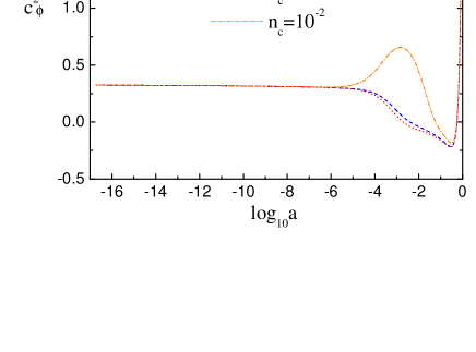
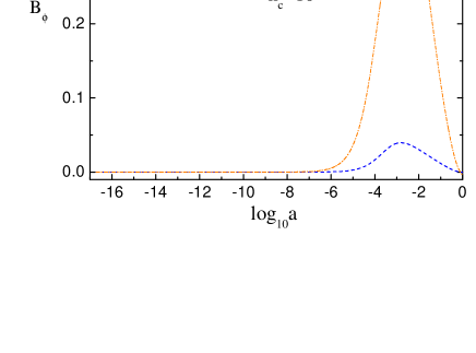
Figure 2: (a) Cosmological evolution of the adiabatic sound speed $c_{\phi}^{2}$ of the scalar field for different values of $n_{c}=0$ (dotted line), $n_{c}=10^{-3}$ (dashed line), and $n_{c}=10^{-2}$ (dash-dotted line) when $\lambda=5$. (b) Behavior of the coupling modification, ${\cal B}_{\phi}$ as a function of the scale factor $a$ for different values of $n_{c}$.

3.1 Isocurvature condition

Due to the out of thermal equilibrium nature of the quintessence, we need to check the isocurvature evolution of the scalar field perturbation [24]. We can analytically show this in the tracking region. First of all the adiabatic sound speed squared $c_{\phi}^{2}$ of the quintessence can be represented as

$$c_{\phi}^{2}=\frac{\bar{p}_{\phi}^{\prime}}{\bar{\rho_{\phi}}^{\prime}}=1+\frac{2\bar{\phi}^{\prime}V_{,\bar{\phi}}}{3{\cal H}(\bar{\rho}_{\phi}+\bar{p}_{\phi})(1-{\cal B}_{\phi})}=\omega_{\phi}-\frac{\omega_{\phi}^{\prime}}{3{\cal H}(1+\omega_{\phi})(1-{\cal B}_{\phi})},$$ (3.15)

where we have used Eq. (2.13). From this equation we can find the second derivative of the potential,

$$\frac{a^{2}}{\bar{M}^{2}}V_{,\bar{\phi}\bar{\phi}}=\frac{3}{2}{\cal H}c_{\phi}^{2^{\prime}}(1-{\cal B}_{\phi})+\frac{3}{2}{\cal H}^{2}(c_{\phi}^{2}-1)(1-{\cal B}_{\phi})\Bigl{[}\frac{{\cal H}^{\prime}}{{\cal H}^{2}}-1-\frac{3}{2}(c_{\phi}^{2}+1)(1-{\cal B}_{\phi})\Bigr{]}-\frac{3}{2}{\cal H}(c_{\phi}^{2}-1){\cal B}_{\phi}^{\prime}.$$ (3.16)

The relation between ${\cal H}^{2}$ and ${\cal H}^{\prime}$ can be found from Eq. (2.35) :

$$\frac{{\cal H}^{\prime}}{{\cal H}^{2}} = -\frac{1}{2}(1+3\omega_{\rm{tot}}),$$ (3.17)

$$\omega_{\rm{tot}} = \sum_{\beta}\omega_{\beta}\Omega_{\beta},$$ (3.18)

where $\omega_{\rm{tot}}$ is the weighted EOS. As long as we use the background as shown in the pervious model, the tracking region is well established during the radiation dominated era [20]. During this era we can find the following relation,

$$c_{\phi}^{2}=\frac{\bar{p}_{\phi}^{\prime}}{\bar{\rho}_{\phi}^{\prime}}=\omega_{\phi}=\omega_{r}.$$ (3.19)

This is shown in the first panel of Fig. 2. As the coupling is increased we can have the non-monotonic behavior of $c_{\phi}^{2}$ as shown in the $n_{c}=10^{-2}$ case. In addition, we can rewrite the coupling term as

$${\cal B}_{\phi}=-\frac{B_{c,\bar{\phi}}\bar{\phi}^{\prime}\bar{\rho}_{c}}{3{\cal H}(\bar{\rho}_{\phi}+\bar{p}_{\phi})}=-\frac{{\cal H}}{\bar{\phi}^{\prime}}B_{c,\bar{\phi}}\bar{\Omega}_{c}.$$ (3.20)

As shown in the second panel of Fig. 2, this term is negligible during the radiation dominated epoch. The coupling drives a faster evolution of $\phi$ when matter energy dominates the Universe and the magnitude of ${\cal B}_{\phi}$ depends on the energy density of the CDM. With these facts we can have the approximate expression of Eq. (3.16),

$$\frac{a^{2}}{\bar{M}^{2}}V_{,\bar{\phi}\bar{\phi}}\simeq\frac{3}{2}{\cal H}^{2}(c_{\phi}^{2}-1)\Bigl{[}\frac{{\cal H}^{\prime}}{{\cal H}^{2}}-\frac{3}{2}(c_{\phi}^{2}+1)\Bigr{]}=-\frac{3}{4}{\cal H}^{2}(c_{\phi}^{2}-1)\Bigl{[}3\omega_{\rm{tot}}+3c_{\phi}^{2}+4\Bigr{]},$$ (3.21)

where we have used Eq. (3.17) in the second equality. The isocurvature mode in the radiation dominated epoch can be obtained from Eq. (2.41) and using the fact that $a\propto\eta$ during the radiation dominated era. To check this we can put $\Phi=0$ and then we have

$$\delta\phi^{\prime\prime}+\frac{4}{(3\omega_{r}+1)\eta}\delta\phi^{\prime}+\Bigl{[}k^{2}-(c_{\phi}^{2}-1)\frac{3}{(3\omega_{r}+1)^{2}\eta^{2}}(3\omega_{r}+3c_{\phi}^{2}+4)\Bigr{]}\delta\phi=0.$$ (3.22)

If we use the tracking solution (3.19), then we can rewrite the above equation as

$$\delta\phi^{\prime\prime}+\frac{2}{\eta}\delta\phi^{\prime}+\Bigl{[}k^{2}+\frac{3}{\eta^{2}}\Bigr{]}\delta\phi=0.$$ (3.23)

The solutions of this equation are Bessel functions,

$$\delta\phi(\eta)={\rm const}~{}\eta^{-1/2}~{}J_{\pm|i\sqrt{11}/2|}(k\eta).$$ (3.24)

Thus both solutions decay in time. At the superhorizon scale the $k$-dependent term can be neglected and we obtain the power-law solutions, $\delta\phi\propto\eta^{\nu}$, where the power index $\nu=(-1\pm i\sqrt{11})/2$. Therefore, any initial nonzero isocurvature fluctuation of the quintessence is damped to zero with time. We will use only the adiabatic perturbations in the following section.

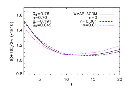
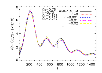
Figure 3: (a) CMB large-scale anisotropy power spectra of $\Lambda$CDM (solid line), minimally coupled $n_{c}=0$ (dotted line), and non-minimally coupled $n_{c}=10^{-3},10^{-2}$ (dashed, dash-dotted line respectively) quintessence models. (b) Same spectra for the entire scales.

4 Effects of coupling

The non-minimally coupled quintessence models have been investigated as a possible solution for the late time coincidence problem [11]. The coupling gives rise to the additional mass and source terms of the evolution equations for CDM and scalar field perturbations. This also affects the perturbation of radiation indirectly through the background bulk ${\cal H}$ and the metric perturbations [25]. The value of the energy density contrast of the CDM ($\Omega_{c}$) is increased in the past when the coupling is increased.

4.1 CMB

The temperature anisotropy measured in a given direction of the sky can be expanded in spherical harmonics as

$$\Theta\equiv\frac{\Delta T}{T}(\hat{n})=\sum_{\ell m}a_{\ell m}Y_{\ell m}(\hat{n}),$$ (4.1)

where $\Theta$ is the temperature brightness function that is the fractional perturbation of the temperature of the photons $T=T_{0}(1+\Theta)$, $\hat{n}$ is the direction of the photon momentum, and $a_{\ell m}$ are the multipoles. We can also expand the brightness function as a Legendre polynomial, $P_{\ell}$ :

$$\Theta=\sum_{\ell}(-i)^{\ell}\,(2\ell+1)\,\Theta_{\ell}\,P_{\ell}.$$ (4.2)

From the inflationary scenario, the multipoles are Gaussian random variables which satisfy

$$\langle a^{*}_{\ell m}\,a_{\ell^{\prime}m^{\prime}}\rangle=C_{\ell}\,\delta_{\ell\ell^{\prime}}\,\delta_{mm^{\prime}}.$$ (4.3)

The angular power spectrum ($C_{\ell}$) contains all the information about the statistical properties of CMB and is defined as [26]

$$\frac{2\ell+1}{4\pi}C_{\ell}=\frac{1}{2\pi^{2}}\int d\eta\frac{dk}{k}\frac{k^{3}|\Theta_{\ell}(k,\eta)|^{2}}{2\ell+1}.$$ (4.4)

In the standard recombination model the acoustic oscillations will be frozen into the CMB. A generalization of the free-streaming equation in a flat universe gives the resulting anisotropies :

$$\frac{\Theta_{\ell}(\eta)}{2\ell+1}=[\Theta_{0}+\Psi](\eta_{ls})j_{\ell}(k(\eta-\eta_{ls}))+\Theta_{1}(\eta_{ls})\frac{1}{k}\frac{d}{d\eta}j_{\ell}(k(\eta-\eta_{ls}))+\int_{\eta_{\,ls}}^{\eta}(\Psi^{\prime}-\Phi^{\prime})j_{\ell}(k(\eta-\tilde{\eta}))d\tilde{\eta}$$ (4.5)

where $j_{\ell}$ is the spherical Bessel function and $\eta_{\,ls}$ is the conformal time at last scattering. Photon density perturbation is related to the temperature perturbation in the matter rest frame :

$$\delta_{r}=4\Theta_{0}+4{\cal H}\frac{\theta_{\rm{tot}}}{k^{2}},$$ (4.6)

and the gravitational potentials will be given in Eq. (5.1) - (5.4) in the following section. We use the fact that in the absence of anisotropic stress, the two scalar potentials $\Psi$ and $\Phi$ defined in the conformal Newtonian gauge (2.1) are equal and they coincide with the usual gravitational potential in the Newtonian limit.

Now, we investigate the effects of non-minimal coupling of a scalar field to the CDM on the CMB power spectrum. Firstly, the Newtonian potential at late times changes more rapidly as the coupling increases, as shown in Eq. (5.1). This leads to an enhanced ISW effect as indicated in the last term of Eq. (4.5). Thus we have a relatively larger $C_{\ell}$ at large scales (i.e. small $\ell$). Thus, if the CMB power spectrum normalized by COBE, then we will have smaller quadrupole [27]. This is shown in the first panel of Fig. 3. One thing that should be emphasized is that we use different parameters for the $\Lambda$CDM and the coupled quintessence models to match the amplitude of the first CMB anisotropy peak. The parameter used for the quintessence model is indicated in Fig. 3 (i.e. $\Omega_{\phi}^{(0)}=0.76$, $\Omega_{m}^{(0)}=0.191$, $\Omega_{b}^{(0)}=0.049$, and $h=0.7$, where $h$ is the present Hubble parameter in the unit of $100{\rm kms^{-1}Mpc^{-1}}$). However, these parameters are well inside the $1\,\sigma$ region given by the WMAP data. We use the WMAP parameters for the $\Lambda$CDM model (i.e. $\Omega_{\phi}^{(0)}=0.73$, $\Omega_{m}^{(0)}=0.23$, $\Omega_{b}^{(0)}=0.04$, and $h=0.72$). In both models we use the same spectral index $n_{s}=1$. The heights of the acoustic peaks at small scales (i.e large $\ell$) can be affected by the following two factors. One is the fact that the scaling of the CDM energy density deviates from that of the baryon energy density. Therefore for the given CDM and baryon energy densities today, the energy density contrast of baryons at decoupling ($\Omega_{b}^{(ls)}$) is getting lower as the coupling is being increased. This suppresses the amplitude of compressional (odd number) peaks while enhancing rarefaction (even number) peaks. The other is that for models normalized by COBE, which approximately fixes the spectrum at $\ell\simeq 10$, the angular amplitude at small scales is suppressed in the coupled quintessence. This is shown in the second panel of Fig. 3. The third peak in this model is smaller than that in the $\Lambda$CDM model. The WMAP data do not show the value of the third peak but quote a compilation of other experiments [28]. The ratio of the amplitude between the second and the third peaks is $1.03\pm 0.02$. In the $\Lambda$CDM model this value is $0.986$ and in our model these values are $1.08$ and $1.11$ for without and with the coupling equal to $n_{c}=0.01$ respectively. We also show the $n_{c}=0.02$ case in this figure. With the same parameters this case can be ruled out from the current data. In all cases, we have used the CMBFAST code [29] with the modified Boltzmann equations to compute the CMB power spectrum.

Secondly, for $\ell>200$ we can see that the locations of the acoustic peaks are slightly shifted to smaller scales (i.e. larger $\ell$). This can be explained as follows. The locations of peaks and troughs can be parametrized as

$$\ell_{m}=\ell_{A}(m-\varphi_{m})=\ell_{A}(m-\bar{\varphi}-\delta\varphi_{m}),$$ (4.7)

where $\ell_{A}$ is the acoustic scale dependent on the geometry of the Universe, $\bar{\varphi}$ is the overall peak shift, and $\delta\varphi_{m}$ is the relative shift of the $m$-th peak relative to the first one [6]. The overall peak shift, $\bar{\varphi}$ is given by

$$\bar{\varphi}\simeq 0.267\Bigl{(}\frac{r_{ls}}{0.3}\Bigr{)}^{0.1},$$ (4.8)

where $r_{ls}=\rho_{r}^{(ls)}/\rho_{m}^{(ls)}$ is the ratio of the energy densities of radiation to matter at last scattering. The shift is due to both driving effects from the decay of the gravitational potential and contributions from the Doppler shift of the oscillating fluid. The acoustic scale $\ell_{A}$ depends on both the sound horizon $s_{ls}$ at decoupling and the angular diameter distance $D$ to the last scattering surface:

$$\ell_{A}=\pi\frac{D}{s_{ls}}=\pi\frac{\eta_{0}-\eta_{\,ls}}{\bar{c}_{s}\eta_{\,ls}},$$ (4.9)

where $\bar{c}_{s}$ is the average sound speed before last scattering :

$$\bar{c}_{s}={\eta}_{\,ls}^{-1}\int_{0}^{\eta_{\,ls}}c_{s}d\eta\hskip 14.45377pt{\rm with}\hskip 14.45377ptc_{s}^{-2}=3+\frac{9}{4}\frac{\rho_{b}}{\rho_{r}}.$$ (4.10)

Also from the Hubble parameter,

$$\Biggl{(}\frac{da}{d\eta}\Biggr{)}^{2}=H_{0}^{2}\Biggl{\{}\Omega_{r}^{(0)}+\Omega_{b}^{(0)}a+\Omega_{m}^{(0)}a^{1+\xi}+\frac{\rho_{\phi}}{\rho_{cr}^{(0)}}a^{4}\Biggr{\}},$$ (4.11)

where $H_{0}$ is the present value of the Hubble parameter, we can find the angular diameter distance,

$$D=\eta_{0}-\eta_{ls}=H_{0}^{-1}\int_{a_{ls}}^{a^{(0)}}\frac{da}{\sqrt{\Omega_{r}^{(0)}+\Omega_{b}^{(0)}a+\Omega_{m}^{(0)}a^{1+\xi}+\rho_{\phi}/\rho_{cr}^{(0)}a^{4}}}.$$ (4.12)

The sound horizon is not affected by the coupling and the effect of coupling on the angular diameter distance is also quite small in our model. However, the overall shift and the relative shift are affected by the coupling. As the coupling is increased, the value of $r_{ls}$ is decreased. Hence, the locations of the peaks are shifted to the right. However, this shift is quite small. We show this in the second panel of Fig. 3. The heights and the locations of the acoustic peaks in various models are summarized in Table 1. There is a significant difference for the heights of the peaks of the second and the third peaks between the models. Thus upcoming observations continuing to focus on resolving the higher peaks may constrain the strength of the coupling.

Table 1: Summary of the heights and the locations of the considered models. The heights of peaks, $A_{i}$ have been scaled by a factor of $10^{10}$. $A_{i:j}$ is the ratio of the $i$-th peak height to the $j$-th. The locations of peaks, $\ell_{i}$.

Model	$A_{1}$	$A_{2}$	$A_{3}$	$\ell_{1}$	$\ell_{2}$	$\ell_{3}$	$A_{1:2}$	$A_{2:3}$
$\Lambda$CDM	$7.26$	$3.25$	$3.30$	$220$	$536$	$812$	$2.23$	$0.986$
$n_{c}=0$	$7.04$	$3.23$	$3.00$	$217$	$532$	$811$	$2.18$	$1.08$
$n_{c}=10^{-2}$	$7.02$	$3.36$	$3.03$	$218$	$535$	$818$	$2.09$	$1.11$

4.2 Matter power spectrum

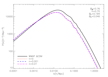
Figure 4: Matter power spectra for the models using the same parameters in Fig. 3.

The effects of quintessence on structure formation in several other models have been investigated [30, 31]. Structure as a function of physical scale size is usually described in terms of a power spectrum :

$$P(k)=\langle|\delta_{k}|^{2}\rangle=Ak^{n_{s}}T^{2}(k),$$ (4.13)

where $A$ is the COBE normalization, $n_{s}$ is a power index, and $T(k)$ is the transfer function. The coupling of quintessence to the CDM can change the shape of matter power spectrum because the location of the turnover corresponds to the scale that entered the Hubble radius when the Universe became matter-dominated. This shift on the scale of matter and radiation equality is indicated in the second panel of Fig. 1:

$$a_{eq}\simeq\frac{\rho_{r}^{(0)}}{\rho_{c}^{(0)}}\exp[B_{c}(\phi_{0})-B_{c}(\phi_{eq})],$$ (4.14)

where $\rho_{r}^{(0)}$ and $\rho_{c}^{(0)}$ are the present values of the energy densities of radiation and CDM respectively, and the approximation comes from the fact that the present energy density of CDM is bigger than that of baryons ($\rho_{c}^{(0)}>\rho_{b}^{(0)}$). Increasing the coupling shifts the epoch of matter-radiation equality further from the present, thereby moving the turnover in the power spectrum to smaller scale. If we define $k_{eq}$ as the wavenumber of the mode which enters the horizon at radiation-matter equality, then we will obtain

$$k_{eq}=\frac{2\pi}{\eta_{eq}}.$$ (4.15)

However, from the previous subsection, we notice that the value of $\eta_{eq}$ remains unchanged for different couplings and this degeneracy is indicated in Fig. 4. We have used different parameters for the $\Lambda$CDM and quintessence models; the matter power spectra look different between the models. There is a slight suppression in the quintessence models. Note that a bias factor could resolve the discrepancy and perhaps a parameter fitting may also help this. However, the detailed parameter fitting is beyond the scope of this paper.

We can write the equation of the matter fluctuation in the synchronous gauge during the matter dominated epoch :

$$\bar{\delta}_{c}^{\prime\prime}+{\cal H}\bar{\delta}_{c}^{\prime}-\frac{3}{2}{\cal H}^{2}\frac{(\delta\bar{\rho}_{c}+\delta\bar{p}_{c})}{\bar{\rho}_{cr}}-\frac{(aF(\phi))^{\prime}}{a}=0,$$ (4.16)

where the coupling term $F(\phi)$ is given by

$$F(\phi)=B_{c,\bar{\phi}\bar{\phi}}\bar{\phi}^{\prime}\delta\phi+B_{c,\bar{\phi}}\delta\phi^{\prime}=n_{c}\lambda(\bar{\phi}\delta\phi)^{\prime}.$$ (4.17)

This equation can be rewritten by the structure growth exponent $f$, which is defined as

$$f(a)=\frac{d\ln\bar{\delta}_{c}(a)}{dx}.$$ (4.18)

Hence, we have the following equation for $f(a)$ which is identical to Eq. (4.16):

$$\frac{df}{dx}+f^{2}+\Bigl{(}2+\frac{d\ln({\cal H}/a)}{dx}\Bigr{)}f-\frac{3}{2}\Omega_{c}=\frac{d\Bigl{[}aF(\phi)\Bigr{]}}{dx}\frac{1}{a{\cal H}\bar{\delta}_{c}},$$ (4.19)

If we use Eq. (2.16), then we can find that $a\propto\eta^{2/(1-\xi)}$ and ${\cal H}=2/(1-\xi)\eta^{-1}$ for a matter dominated universe. As we can see from the above Eq. (4.19) that the coupling term is negligible because $\phi$ varies much slower than ${\cal H}$. Thus we can ignore the last term in Eq. (4.16). From this we can rewrite the above equation in a matter dominated era :

$$\bar{\delta}_{c}^{\prime\prime}+\frac{2}{(1-\xi)\eta}\bar{\delta}_{c}^{\prime}-\frac{6}{(1-\xi)^{2}\eta^{2}}\bar{\delta}_{c}=0.$$ (4.20)

This equation has two solutions,

$$\bar{\delta}_{c}^{\pm}=c_{\pm}\eta^{\nu_{\pm}},$$ (4.21)

where $c_{\pm}$ are arbitrary constants and

$$\nu_{\pm}=\frac{-(1+\xi)\pm\sqrt{24+(1+\xi)^{2}}}{2(1-\xi)}.$$ (4.22)

$\bar{\delta}_{c}^{+}$ indicates a growing mode, which is only relevant today because $|\bar{\delta}_{c}^{+}|$ is small at early time and we can ignore the decaying mode $\bar{\delta}_{c}^{-}$. If we remove the coupling effect in this solution, then we can recover the well known solution $\delta_{c}^{+}=\eta^{2/3}$. This effect is shown in Fig. 4.

As the coupling is increased, we have little more matter at early times and this increases the height of the matter power spectrum. Again this effect is tiny and we can hardly see the difference between various couplings.

5 Metric perturbation

In addition to these, the perturbed equations of the metric can be obtained from the Einstein equations:

$$k^{2}\Phi+3{\cal H}\Bigl{(}\Phi^{\prime}+{\cal H}\Psi\Bigr{)} = \frac{3}{2}\frac{{\cal H}^{2}}{\bar{\rho}_{tot}}\delta T^{0}_{(tot)0},$$ (5.1)

$$\Phi^{\prime\prime}+{\cal H}(\Psi^{\prime}+2\Phi^{\prime})+\Bigl{(}2{\cal H}^{\prime}+{\cal H}^{2}\Bigr{)}\Psi+\frac{k^{2}}{3}(\Phi-\Psi) = \frac{1}{2}\frac{{\cal H}^{2}}{\bar{\rho}_{tot}}\delta T^{i}_{(tot)i},$$ (5.2)

$$k^{2}\Bigl{(}\Phi^{\prime}+{\cal H}\Psi\Bigr{)} = \frac{3}{2}{\cal H}^{2}\sum_{\beta}(1+\omega_{\beta})\bar{\Omega}_{\beta}\theta_{\beta},$$ (5.3)

$$k^{2}(\Phi-\Psi) = \frac{9}{2}{\cal H}^{2}\sum_{\beta}(1+\omega_{\beta})\bar{\Omega}_{\beta}\sigma_{\beta},$$ (5.4)

where we have used the unperturbed equations (2.34) and (2.35) . From Eqs. (5.1) and (5.2), we can find the metric perturbation equation,

$$\Phi^{\prime\prime}+{\cal H}(\Psi^{\prime}+5\Phi^{\prime})+2({\cal H}^{\prime}+2{\cal H}^{2})\Psi+\frac{k^{2}}{3}(4\Phi-\Psi)$$

$$=-\frac{a^{2}}{2\bar{M}^{2}}[(1-c_{tot}^{2})\delta\rho_{tot}-p_{tot}\Gamma_{int}-p_{tot}\Gamma_{rel}].$$ (5.5)

If we use Eq. (5.1), this equation can be rewritten as

$$\Phi^{\prime\prime}+{\cal H}\Bigl{[}\Psi^{\prime}+(2+3c_{tot}^{2})\Phi^{\prime}\Bigr{]}+\Bigl{[}2{\cal H}^{\prime}+{\cal H}^{2}(1+3c_{tot}^{2})\Bigr{]}\Psi+\frac{k^{2}}{3}\Bigl{[}(1+3c_{tot}^{2})\Phi-\Psi\Bigr{]}$$

$$=\frac{a^{2}}{2\bar{M}^{2}}\Bigl{(}p_{tot}\Gamma_{int}+p_{tot}\Gamma_{rel}\Bigr{)}\equiv\frac{a^{2}}{2\bar{M}^{2}}p_{tot}\Gamma_{tot},$$ (5.6)

where we define $\Gamma_{tot}=\Gamma_{int}+\Gamma_{rel}$ in the last equality. The last term in this equation comes from the coupling of the scalar field. So even if we start from the adiabatic condition ( $p_{tot}\Gamma_{tot}=0$), we can analytically solve the above equation for the specific case. Let us first put $\Psi=\Phi$ (no anisotropic stress) and $k^{2}c_{tot}^{2}\Phi=0$ (consider the superhorizon scale), then Eq. (5.6) is simplified as

$$\Phi^{\prime\prime}+3{\cal H}(1+c_{tot}^{2})\Phi^{\prime}+\Bigl{[}2{\cal H}^{\prime}+{\cal H}^{2}(1+3c_{tot}^{2})\Bigr{]}\Phi=\frac{a^{2}}{2\bar{M}^{2}}p_{tot}\Gamma_{tot}.$$ (5.7)

If you use the background equations, this equation can be rewritten as

$$\Phi^{\prime\prime}-\Bigl{(}\ln[\rho_{tot}+p_{tot}]\Bigr{)}^{\prime}\Phi^{\prime}+\Bigl{(}\ln[\rho_{tot}/(\rho_{tot}+p_{tot})]\Bigr{)}^{\prime}{\cal H}\Phi=\frac{3{\cal H}^{2}}{2}\frac{p_{tot}}{\rho_{tot}}\Gamma_{tot}.$$ (5.8)

If we consider the adiabatic condition ($p_{tot}\Gamma_{tot}=0$), then the above equation is identical to the equation in Bardeen’s article [32].As such, the metric perturbation can be rewritten as the curvature perturbation [33],

$$\zeta=\frac{({\cal H}^{-1}\Phi^{\prime}+\Phi)}{(1+\omega_{tot})}+\frac{3}{2}\Phi.$$ (5.9)

With this we can express Eq. (5.7) in the adiabatic case as

$$\zeta^{\prime}=0.$$ (5.10)

This result looks the same to the minimally coupled case and there seems to have no difference from the non-minimally coupled case. Nevertheless, the coupling information is absorbed in both $c_{tot}^{2}$ and the perturbation equation of each species.

6 Conclusions

We have analyzed the linear perturbations of the cosmological models for the scalar field with its self-interaction potential, $V(\phi)=V_{0}\exp(\lambda\phi^{2}/2)$, and its coupling to the CDM, $\exp[B_{c}(\phi)]=\exp(n_{c}\lambda\phi^{2}/2)$. The evolution of the non-perturbed background scalar field $\bar{\phi}$ occurred in the tracking regime throughout the radiation dominated epoch. The full analysis of the non-perturbed and perturbed equation of each species in the conformal Newtonian gauge has been done including the proper energy-momentum transfer vector due to the coupling, $Q_{(d)\nu}$. The Boltzmann equations have been modified as to account for the coupling between a scalar field and the CDM.

We have seen that the energy-momentum of each species may not be conserved as a result of the coupling of the scalar field to the CDM. Thus we have redefined the concepts of entropy perturbations. We have shown that the isocurvature perturbation of the quintessence has been damped to zero with time in the tracking regime during the radiation epoch. Thus we have constrained our considerations on the adiabatic perturbation.

We have considered the CMB anisotropy spectrum and the matter power spectrum for the non-minimally coupled models. Additional mass and source terms in the Boltzmann equations induced by the coupling give the rapid changes of the Newtonian potential $\Phi$ and enhance the ISW effect in the CMB power spectrum. The modification of the evolution of the CDM, $\rho_{c}=\rho_{c}^{(0)}a^{-3+\xi}$, changes the energy density contrast of the CDM at early epoch. We have adopted the current cosmological parameters measured by WMAP within $1\sigma$ level. With the COBE normalization and the WMAP data we have found the constraint of the coupling $n_{c}\leq 0.01$. The locations and the heights of the CMB anisotropy peaks have been changed due to the coupling. Especially, there is a significant difference for the heights of the second and the third peaks among the models. Thus upcoming observations continuing to focus on resolving the higher peaks may constrain the strength of the coupling. The suppression of the amplitudes of the matter power spectra could be lifted by a bias factor. However, a detailed fitting is beyond the scope of this paper. The turnover scale of the matter power spectrum may be used to constrain the strength of the coupling $n_{c}$.

Finally, we have investigated the metric perturbations including the coupling between the scalar field and the CDM. There is no difference to the curvature perturbation $\zeta$ for the different couplings in the adiabatic case. However, the effects of the coupling have been absorbed in the Boltzmann equations already.

7 Acknowledgements

This work was supported in part by the National Science Council, Taiwan, ROC under the Grant NSC94-2112-M-001-024 (K.W.N.).

References

- [1] A. G. Riess et al. [Supernova Search Team Collaboration], Astron. J. 116, 1009 (1998) [astro-ph/9805201]; Astrophys. J. 607, 665 (2004) [astro-ph/0402512]; S. Perlmutter et al. [Supernova Cosmology Project Collaboration], Astrophys. J. 517, 565 (1999) [astro-ph/9812133]; N. A. Bahcall, J. P. Ostriker, S. Perlmutter, and P. J. Steinhardt, Science 284, 1481 (1999) [astro-ph/9906463]; T. Padmanabhan and T. R. Choudhury, Mon. Not. Roy. Astron. Soc. 344, 823 (2003) [astro-ph/0212573]; Astron. Astrophys. 429, 807 (2005) [astro-ph/0311622]; P. Astier et al., [astro-ph/0510447].
- [2] C. L. Bennett et al., Astrophys. J. Suppl . Ser 148, 1 (2003) [astro-ph/0302207]; D. N. Spergel et al., Astrophys. J. Suppl. Ser. 148, 175 (2003) [astro-ph/0302209].
- [3] M. Tegmark et al., Phys. Rev. D 69, 103501 (2004) [astro-ph/0310723].
- [4] M. Colless et al., Mon. Not. Roy. Astron. Soc. 328, 1039 (2001) [astro-ph/0106498]; [astro-ph/0306581].
- [5] R. R. Caldwell, R. Dave, and P. J. Steinhardt, Phys. Rev. Lett 80, 1582 (1998) [astro-ph/9708069].
- [6] M. Doran, M. J. Lilley, J. Schwindt, and C. Wetterich, Astrophys. J. 559, 501 (2001) [astro-ph/0012139]; M. Doran and M. J. Lilley, Mon. Not. Roy. Astron. Soc. 330, 965 (2002) [astro-ph/0104486]; W. Lee and K.-W. Ng, Phys. Rev. D 67, 107302 (2003) [astro-ph/0209093].
- [7] S. Lee, Phys. Rev. D 71, 123528 (2005) [astro-ph/0504650].
- [8] R. K. Sachs and A. M. Wolfe, Astrophys. J. 147, 73 (1967).
- [9] K. Coble, S. Dodelson, and J. A. Frieman, Phys. Rev. D 55, 1851 (1997) [astro-ph/9608122].
- [10] B. Ratra and P. J. E. Peebles, Phys. Rev. D 37, 3406 (1988); Astrophys. J. 325, L117 (1988); C. Wetterich, Nucl. Phys. B 302, 668 (1988); P. G. Ferreira and M. Joyce, Phys. Rev. D 58, 023503 (1998) [astro-ph/9711102].
- [11] J. P. Uzan, Phys. Rev. D 59, 123510 (1999) [gr-qc/9903004]; L. Amendola, Phys. Rev. D 62, 043511 (2000) [astro-ph/9808023]; W. Zimdahl, D. Pavn, and L. P. Chimento, Phys. Lett. B 521, 133 (2001) [astro-ph/0105479]; D. Tocchini-Valentini and L. Amendola, Phys. Rev. D 65, 063508 (2002) [astro-ph/0108143]; D. Pavn, Gen. Relativ. Grav. 35, 413 (2003) [astro-ph/0210484]; L. P. Chimento, A. S. Jakubi, D. Pavn, and W. Zimdahl, Phys. Rev. D 67, 083513 (2003) [astro-ph/0303145]; D. Pavn, S. Sen, and W. Zimdahl, J. Cosmol. Astropart. Phys. 05 (2004) 9 [astro-ph/0402067]; G. Olivares, F. Atrio-Barandela, and D. Pavn, Phys. Rev. D 71, 063523 (2005) [astro-ph/0503242].
- [12] M. B. Hoffman [astro-ph/0307350]; T. Koivisto, Phys. Rev. D 72, 043516 (2005) [astro-ph/0504571].
- [13] M. Kawasaki, T. Moroi, and T. Takahashi, Phys. Rev. D 64, 083009 (2001) [astro-ph/0105161].
- [14] V. F. Mukhanov, H. A. Feldman, and R. H. Brandenberger, Phys. Rep. 215, 203 (1992).
- [15] L. Amendola, Phys. Rev. D 60, 043501 (1999) [astro-ph/9904120].
- [16] T. Damour, G. W. Gibbons, and C. Gundlach, Phys. Rev. Lett. 64, 123 (1990); T. Damour and C. Gundlach, Phys. Rev. D 43, 3873 (1991).
- [17] T. Damour and K. Nordtvedt, Phys. Rev. Lett. 70, 2217 (1993); Phys. Rev. D 48, 3436 (1993); T. Damour and A. M. Polyakov, Nucl. Phys. B 423, 532 (1994); Gen. Relativ. Gravit. 26, 043511 (1994).
- [18] R. Bean and J. Magueijo, Phys. Lett. B 517, 177 (2001) [astro-ph/0007199], L. Amendola and D. Tocchini-Valentini, Phys. Rev. D 64, 043509 (2001) [asstro-ph/0011243].
- [19] P. J. E. Peebles, Principles of Physical Cosmology (Princeton University Press, Princeton, 1993).
- [20] S. Lee, K. A. Olive, and M. Pospelov, Phys. Rev. D 70, 083503 (2004) [astro-ph/0406039].
- [21] H. Kodama and M. Sasaki, Prog. Theor. Phys. Suppl. 78, 1 (1984).
- [22] R. Bean, S. H. Hansen, and A. Melchiorri, Phys. Rev. D 64, 103508 (2001) [astro-ph/0104162].
- [23] C.-P. Ma and E. Bertschinger, Astrophys. J. 455, 7 (1995) [astro-ph/9506072].
- [24] P. Brax, J. Martin, and A. Riazuelo, Phys. Rev. D 62, 103505 (2000) [astro-ph/0005428]; L. R. Abramo and F. Finelli, Phys. Rev. D 64, 083513 (2001) [astro-ph/0101014]; M. Kawasaki, T. Moroi, and T. Takahashi, Phys. Lett. B 533, 294 (2002) [astro-ph/0108081].
- [25] R. Bean, Phys. Rev. D 64, 123516 (2001) [astro-ph/0104464].
- [26] W. Hu and N Sugiyama, Phys. Rev. D 51, 2599 (1995) [astro-ph/9407093].
- [27] M. White and E. F. Bunn, Astrophys. J 450, 477 (1995); Erratum-ibid. 477, 460 (1995) [astro-ph/9503054].
- [28] X. Wang, M. Tegmark, B. Jain, and M. Zaldarriaga, Phys. Rev. D 68, 123001 (2003) [astro-ph/0212417].
- [29] U. Seljak and M. Zaldarriaga, Astrophys. J 469, 437 (1996) [astro-ph/9603033].
- [30] L. Wang and P. J. Steinhardt, Astrophys.J 508, 483 (1998) [astro-ph/9804015].
- [31] C. Skordis and A. Albrecht, Phys. Rev. D 66 043523 (2002) [astro-ph/0012195]; M. Doran, J. M. Schwindt, and C. Wetterich, Phys. Rev. D 64, 123520 (2001) [astro-ph/0107525]; M. Kunz, P. S. Corasaniti, D. Parkinson, and E. J. Copeland, Phys. Rev. D 70, 041301 (2004) [astro-ph/0307346]; C. Horellou and J. Berge, Mon. Not. Roy. Astron. Soc 360 1393 (2005) [astro-ph/0504465].
- [32] J. Bardeen, Phys. Rev. D 22, 1882 (1980) .
- [33] D. Lyth, Phys. Rev. D 31, 1792 (1985) .