Nonlinear perturbations for dissipative and interacting relativistic fluids

Abstract

We develop a covariant formalism to study nonlinear perturbations of dissipative and interacting relativistic fluids. We derive nonlinear evolution equations for various covectors defined as linear combinations of the spatial gradients of the local number of e-folds and of some scalar quantities characterizing the fluid, such as the energy density or the particle number density. For interacting fluids we decompose perturbations into adiabatic and entropy components and derive their coupled evolution equations, recovering and extending the results obtained in the context of the linear theory. For non-dissipative and noninteracting fluids, these evolution equations reduce to the conservation equations that we have obtained in recent works. We also illustrate geometrically the meaning of the covectors that we have introduced.

1 Introduction

Recently, we have developed [1, 2] a new formalism for nonlinear relativistic perturbations, based on a covariant approach [3, 4] and inspired by the work of Ellis and Bruni [5]. A key quantity in our formalism is the covector $\zeta_{a}$, a linear combination of the spatial gradients of the energy density $\rho$ and of $\alpha$, the local number of e-folds, or integrated expansion along each worldline of the fluid.

As we showed in [1, 2], $\zeta_{a}$, for a barotropic fluid, obeys a remarkably simple conservation equation, which is exact and fully nonlinear. In the linear approximation, this conservation equation reduces to the usual conservation law for the linear curvature perturbation on uniform energy density hypersurfaces, usually denoted $\zeta$. Thus, our covector $\zeta_{a}$ can be seen as a covariant and nonlinear generalization of the usual $\zeta$.

It must be stressed that, although our initial motivations were related to cosmology, our formalism applies, in fact, to any relativistic fluid, whatever the underlying geometry. Thus, in the following we will not assume any particular type of spacetime, unless specified.

The purpose of the present work is to clarify the geometrical meaning of $\zeta_{a}$, and to extend our formalism in two new directions. Whereas our formalism has been developed so far for a perfect fluid, we consider here its extension to the case of dissipative relativistic fluids. Moreover, we consider the possibility of having several different interacting fluids.

The covariant formalism of Ellis and Bruni [5] was first extended to a dissipative multifluid system in [6, 7], where both the exact and the linear form of perturbation equations were given for noninteracting fluids. It was later generalized to the case of interacting fluids in [8] for linear perturbations.

The extension to interacting fluids is particularly useful in cosmology, where several types of matter coexist. As a typical example, one can mention the analysis of the cosmic microwave background anisotropies, which has been for instance considered within the covariant formalism and at linear order in [9].

In this paper we work in the framework of our nonlinear formalism [1, 2], based on covectors such as $\zeta_{a}$. As in the single perfect fluid case, we show that it is possible to derive simple, exact, and fully nonlinear evolution equations for various covectors, constructed as linear combinations of the spatial gradients of scalar quantities that characterize the fluids, such as the energy density or the number particle, and of the local number of e-folds $\alpha$.

The equations we obtain represent nonlinear generalizations of linear perturbation equations, some of which have been already studied in the context of linear cosmological perturbations (see, in particular, [10, 11]). However, our equations are covariant, i.e., independent of the coordinate system, and nonlinear, and it is straightforward to linearize or expand them up to second, or higher, order in the perturbations. Furthermore, our covariant approach allows to identify easily which properties belong specifically to the linear or second order expansion, and which properties remain valid at higher orders.

This work is organized as follows. In Sec. 2 we introduce the covariant formalism for dissipative fluids while in Sec. 3 we discuss the geometrical meaning of the nonlinear covector $\zeta_{a}$. In Sec. 4 we derive an identity that can be used to construct conservation equations for various nonlinear covectors, representing the perturbations of scalar quantities of a dissipative fluid. The conservation equations for these quantities are derived in Sec. 5, while in Sec. 6 we extend our formalism to interacting fluids. Finally, in Sec. 7, we conclude.

2 Covariant formalism

In this section, we briefly review the covariant description for a dissipative relativistic fluid. There is a substantial literature on dissipative relativistic fluids, which is reviewed, for instance, in [12]. The extension of irreversible thermodynamics to relativistic fluids is hampered by subtle issues. In particular, the first extensions, due to Eckart in 1940 and to Landau and Lifshitz in the 1950’s suffer from non-causal behavior. An extended theory, which does not suffer from this problem was developed by Israel and Stewart [13]. In the present work, we will not need to enter the details of these various formulations and, for details, we refer the reader to [12], whose presentation and notation will be followed here.

We first define the unit four-velocity of the fluid $u^{a}$ as the average velocity of the fluid particles. This means that $u^{a}$ is proportional to the particle current $n^{a}$, which can thus be written as

$$n^{a}=nu^{a},\qquad u^{a}u_{a}=-1,$$ (1)

where $n$ is the particle number density.

In addition to the particle number density $n$, the fluid is characterized by local equilibrium scalars: the energy density $\rho$, the pressure $p$, the entropy $S$ and the temperature $T$. In general the effective pressure deviates from the local equilibrium pressure so that $p_{\rm eff}=p+\Pi$. The energy-momentum tensor can be written in the form

$$T_{ab}=\rho u_{a}u_{b}+\left(p+\Pi\right)h_{ab}+q_{a}u_{b}+q_{b}u_{a}+\pi_{ab},$$ (2)

where $h_{ab}$ is the projection tensor orthogonal to the fluid velocity $u^{a}$,

$$h_{ab}=g_{ab}+u_{a}u_{b},\quad\quad(h^{a}_{\ b}h^{b}_{\ c}=h^{a}_{\ c}\,,\quad h_{a}^{\ b}u_{b}=0),$$ (3)

and where the energy flow $q_{a}$ and the anisotropic stress $\pi_{ab}$ satisfy the following properties:

$$q_{a}u^{a}=0,\quad\pi_{ab}=\pi_{ba},\quad\pi_{a}^{\ a}=0,\quad\pi_{ab}u^{b}=0.$$ (4)

It is useful to introduce the familiar decomposition

$$\nabla_{b}u_{a}=\sigma_{ab}+\omega_{ab}+{1\over 3}\Theta h_{ab}-\dot{u}_{a}u_{b},$$ (5)

with the (symmetric) shear tensor $\sigma_{ab}$, and the (antisymmetric) vorticity tensor $\omega_{ab}$; the volume expansion, $\Theta$, is defined by

$$\Theta\equiv\nabla_{a}u^{a},$$ (6)

while $\dot{u}^{a}$ is the acceleration, with the dot denoting the covariant derivative projected along $u^{a}$, i.e., $\dot{}\equiv u^{a}\nabla_{a}$.

We also introduce the covariant spatial derivative, which is defined as

$$D_{a}\chi\equiv h_{a}^{\ b}\nabla_{b}\chi,\quad\quad D_{a}\chi_{b}=h_{a}^{\ c}h_{b}^{\ d}\nabla_{c}\chi_{d},\quad\quad{\rm etc,}$$ (7)

where $\chi$ and $\chi_{a}$ are a generic scalar and covector, respectively. As illustrated in [5], the covariant spatial derivative is particularly useful to deal with cosmological perturbations in a covariant way, as an alternative to the standard coordinate based approach.

The conservation of the energy-momentum tensor,

$$\nabla_{a}T^{a}_{\ b}=0,$$ (8)

yields, by projection along $u^{a}$, the energy conservation equation,

$$\dot{\rho}+\Theta(\rho+p+\Pi)+\pi^{b}_{\ a}\nabla_{b}u^{a}+\nabla_{a}q^{a}+q^{a}\dot{u}_{a}=0.$$ (9)

Using the decomposition (5) and the definition of the spatial covariant derivative (7), one can rewrite the above equation in the form

$$\dot{\rho}+\Theta(\rho+p)={\cal D},\quad\quad{\cal D}=-\left(\Theta\Pi+\pi^{ab}\sigma_{ab}+D_{a}q^{a}+2q^{a}\dot{u}_{a}\right).$$ (10)

The scalar quantity ${\cal D}$ thus contains all the dissipative terms and vanishes for a perfect fluid.

In irreversible thermodynamics, the entropy is not conserved but increases according to the second law of thermodynamics. This can be expressed by the inequality

$$\nabla_{a}S^{a}\geq 0,$$ (11)

where $S^{a}$ is the entropy current. One usually writes $S^{a}$ in the form

$$S^{a}=Snu^{a}+\frac{R^{a}}{T},$$ (12)

where $R^{a}$ is a dissipative term. As discussed in [12], the explicit form for $R^{a}$ varies according to the formalisms which have been introduced in the literature. The entropy $S$ and temperature $T$ are the local equilibrium quantities, which are related via the Gibbs equation,

$$TdS=d\left(\frac{\rho}{n}\right)+p\,d\left(\frac{1}{n}\right).$$ (13)

This implies, in particular,

$$nT\dot{S}=\dot{\rho}+\Theta\left(\rho+p\right),$$ (14)

where we have assumed conservation of the particle number, i.e.

$$\nabla_{a}n^{a}=0\quad\Leftrightarrow\quad\dot{n}+\Theta n=0.$$ (15)

Using the energy conservation equation (10), this can be rewritten as

$$nT\dot{S}={\cal D}.$$ (16)

In terms of the entropy density $s=nS$, this gives, using once more the particle conservation equation,

$$\dot{s}+\Theta s=\frac{{\cal D}}{T}.$$ (17)

Using this equation, one gets

$$\nabla_{a}S^{a}=\frac{{\cal D}}{T}+\nabla_{a}\left(\frac{R^{a}}{T}\right).$$ (18)

In the case of a non-dissipative fluid, the right hand side is zero and the above relation then expresses the conservation of entropy.

3 Nonlinear covector

Here we illustrate the geometrical meaning of the nonlinear covector that we introduced in [1, 2]. This interpretation can easily be extended to the other covectors of the same form that will be defined in this paper.

As we showed in our recent works [1, 2] (see also [14, 15, 16] for other recent formulations of conserved nonlinear perturbations), a crucial quantity to define conserved nonlinear perturbations is the spatial gradient of the local number of e-folds, $\alpha$, which is defined as the integration of $\Theta$ along the fluid world lines with respect to the proper time $\tau$,

$$\alpha\equiv{1\over 3}\int d\tau\,\Theta.$$ (19)

It follows that

$$\Theta=3\dot{\alpha}=3u^{a}\nabla_{a}\alpha.$$ (20)

In [1, 2], we have introduced, for a perfect fluid, a linear combination of the spatial covariant derivatives of $\alpha$ and $\rho$,

$$\zeta_{a}=D_{a}\alpha-\frac{\dot{\alpha}}{\dot{\rho}}D_{a}\rho.$$ (21)

This covector is fully conserved on all scales for adiabatic perturbations, and can be seen as the nonlinear generalization of the usual $\zeta$. In Sec. 5 we will rederive the conservation equation for this quantity.

At this stage, it is instructive to give a graphical representation of $\zeta_{a}$. To work with a scalar quantity rather than a covector, let us consider an infinitesimal vector $e^{a}$ which is orthogonal to the fluid four-velocity $u^{a}$ at some spacetime point $q$. One can then write

$$e^{a}\zeta_{a}=\Delta\alpha-\frac{\dot{\alpha}}{\dot{\rho}}\Delta\rho,$$ (22)

with

$$\Delta\alpha\equiv e^{a}\nabla_{a}\alpha,\quad\quad\Delta\rho\equiv e^{a}\nabla_{a}\rho.$$ (23)

As shown in Fig. 1, starting from our fiducial reference point $q$, the infinitesimal quantity $\Delta\alpha$ corresponds to the shift in $\alpha$ when one goes from $q$ to the neighboring point $q^{\prime}$ indicated by $e^{a}$. Thus $q^{\prime}$ belongs to the hypersurface $\Sigma_{\alpha+\Delta\alpha}$ characterized by the constant value $\alpha+\Delta\alpha$. Similarly, $q^{\prime}$ belongs to the constant energy density hypersurface $\Sigma_{\rho+\Delta\rho}$. Now, these two hypersurfaces also intersect the fluid worldline that goes through $q$, but in general the intersections differ.

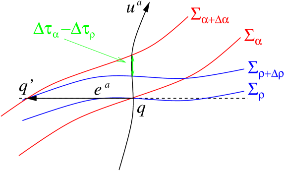
Figure 1: Geometric interpretation of $\zeta_{a}$.

The quantity $e^{a}\zeta_{a}$ quantifies, in terms of the number of e-folds, the separation between these two intersection points. Indeed, the proper time interval between $q$ and the intersection of the hypersurface $\Sigma_{\alpha+\Delta\alpha}$ with the worldline of $q$ is $\Delta\tau_{\alpha}\equiv{\Delta\alpha}/{\dot{\alpha}}$ while the proper time interval between $q$ and the intersection of the hypersurface $\Sigma_{\rho+\Delta\rho}$ with the worldline of $q$ is $\Delta\tau_{\rho}\equiv{\Delta\rho}/{\dot{\rho}}$. The difference between these two proper time intervals is shown in the figure and the corresponding variation of $\alpha$ during this time difference interval is $e^{a}\zeta_{a}=\dot{\alpha}(\Delta\tau_{\alpha}-\Delta\tau_{\rho})$.

4 An identity for nonlinear covectors

In this section we will derive a general identity which we will use later for various cases. Namely, we will show that if one starts with an equation of the form

$$\dot{f}+\Theta g=0,$$ (24)

where $f$ and $g$ are two scalar quantities and, as before, the dot denotes the derivative along $u^{a}$, one finds the identity

$${\cal L}_{u}\left(D_{a}\alpha-\frac{\dot{\alpha}}{\dot{f}}D_{a}f\right)=3\frac{\dot{\alpha}^{2}}{\dot{f}}\left(D_{a}g-\frac{\dot{g}}{\dot{f}}D_{a}f\right).$$ (25)

To show this, let us start by rewriting Equation (24) as

$$\dot{\alpha}+\frac{\dot{f}}{3g}=0.$$ (26)

Taking the spatially projected derivative, one gets

$$D_{a}\dot{\alpha}-\frac{\dot{\alpha}}{\dot{f}}D_{a}\dot{f}+\frac{\dot{\alpha}}{g}D_{a}g=0.$$ (27)

We now wish to invert the time derivative and the spatial gradient. In order to do so, it is convenient to introduce the Lie derivative along $u^{a}$, ${\cal L}_{u}$. Its action on a covector is given by the expression

$${\cal L}_{u}\chi_{a}\equiv u^{c}\nabla_{c}\chi_{a}+\chi_{c}\nabla_{a}u^{c}=u^{c}\partial_{c}\chi_{a}+\chi_{c}\partial_{a}u^{c}.$$ (28)

For a scalar, ${\cal L}_{u}f=\dot{f}$. The Lie derivation along $u^{a}$ and the spatial gradient $D_{a}$ do not commute. Instead, one finds [1, 2]

$$D_{a}\left(\dot{f}\right)={\cal L}_{u}\left(D_{a}f\right)-\dot{u}_{a}\dot{f}.$$ (29)

Applying this identity both to $\alpha$ and $f$, one obtains

$$D_{a}\dot{\alpha}-\frac{\dot{\alpha}}{\dot{f}}D_{a}\dot{f}={\cal L}_{u}\left(D_{a}\alpha\right)-\frac{\dot{\alpha}}{\dot{f}}{\cal L}_{u}\left(D_{a}f\right).$$ (30)

Substituting in (27), one finds

$${\cal L}_{u}\left(D_{a}\alpha-\frac{\dot{\alpha}}{\dot{f}}D_{a}f\right)+{{\left(\frac{\dot{\alpha}}{\dot{f}}\right)}^{\hbox{.}}}D_{a}f-3\frac{\dot{\alpha}^{2}}{\dot{f}}D_{a}g=0,$$ (31)

where we have used Eq. (24) to rewrite the last term. Moreover, Eq. (24) implies

$${{\left(\frac{\dot{\alpha}}{\dot{f}}\right)}^{\hbox{.}}}=3\dot{g}\frac{\dot{\alpha}^{2}}{\dot{f}},$$ (32)

which can be used to rewrite Eq. (31) in the form given in Eq. (25).

For practical purposes, it is useful to note that, for the covectors

$$\zeta_{a}^{(f)}=D_{a}\alpha-\frac{\dot{\alpha}}{\dot{f}}D_{a}f,\qquad\Gamma_{a}^{(g,f)}=D_{a}g-\frac{\dot{g}}{\dot{f}}D_{a}f,$$ (33)

which are defined as very particular linear combinations of spatially projected gradients, one can replace the latter by ordinary gradients and write

$$\zeta_{a}^{(f)}=\partial_{a}\alpha-\frac{\dot{\alpha}}{\dot{f}}\partial_{a}f,\qquad\Gamma_{a}^{(g,f)}=\partial_{a}g-\frac{\dot{g}}{\dot{f}}\partial_{a}f.$$ (34)

This is a consequence of the identity

$$D_{a}\chi=\partial_{a}\chi+u_{a}\dot{\chi},$$ (35)

valid for any scalar quantity $\chi$.

5 Nonlinear (non-)conservation equations

That one can construct conserved cosmological perturbations associated with each quantity whose local evolution is determined entirely by the local expansion of the universe was shown in [14]. There, it was pointed out that such a construction can be extended even in the nonlinear regime, although an explicit expression of the nonlinear perturbation variables was not given.

Here we explicitly construct these variables and their evolution equations. In particular, we use the identity (25) to derive conservation – or non-conservation – equations for various covectors which represent nonlinear perturbations. In this section, we discuss these equations for the nonlinear generalization of the curvature perturbation on hypersurfaces of uniform number density $n$, uniform energy density $\rho$, or uniform entropy density $s$. The corresponding covectors are obtained immediately by replacing the quantity $f$ in Eq. (25) with $n$, $\rho$, or $s$, respectively. As in [1, 2], the curvature perturbation is replaced here by $\alpha$, the local number of e-folds of an observer comoving with the fluid particles.

5.1 Particle conservation

The particle conservation equation,

$$\nabla_{a}(n\,u^{a})=0,$$ (36)

can be rewritten as

$$\dot{n}+\Theta n=0,$$ (37)

which is exactly of the form (24) with $f=g=n$. Equation (25) tells us immediately that the particle conservation law yields, for the covector

$$\zeta_{a}^{(n)}=D_{a}\alpha-{\dot{\alpha}\over\dot{n}}D_{a}n,$$ (38)

the equation

$${\cal L}_{u}\zeta_{a}^{(n)}=0.$$ (39)

This result has already been given in [2].

This can be generalized to the case where the number of particles is not conserved, in which case one can write

$$\nabla_{a}(n\,u^{a})=-\Gamma n,$$ (40)

where $\Gamma$ is the decay rate, which is not supposed to be a constant here. Equivalently, one can write

$$\dot{n}+\Theta n+\Gamma n=0,$$ (41)

which is still of the form (24) with $f=n$ and $g=n+(\Gamma n)/\Theta$. Taking the spatially projected gradients, one thus finds

$${\cal L}_{u}\zeta_{a}^{(n)}=\frac{3\dot{\alpha}^{2}}{\dot{n}}\left(D_{a}\Gamma-\frac{\dot{\Gamma}}{\dot{n}}D_{a}n-D_{a}\Theta+\frac{\dot{\Theta}}{\dot{n}}D_{a}n\right).$$ (42)

The particle annihilation (or production) rate $\Gamma n$ acts here as a source for the evolution of the particle number density perturbation. We will discuss more thoroughly the case of several interacting fluids below in Sec. 6.

5.2 Energy conservation

In the general case, if one introduces the quantity

$$\beta\equiv-\frac{{\cal D}}{\Theta}=(\Theta\Pi+\pi^{ab}\sigma_{ab}+D_{a}q^{a}+2q^{a}\dot{u}_{a})/{\Theta},$$ (43)

then the energy conservation equation (10), becomes

$$\dot{\rho}+\Theta(\rho+p+\beta)=0,$$ (44)

where $\beta$ acts as an extra pressure term, which we will call dissipative pressure.

One can apply the identity derived in the previous section with $f=\rho$ and $g=\rho+p+\beta$. This yields directly

$${\cal L}_{u}\zeta_{a}=\frac{3\dot{\alpha}^{2}}{\dot{\rho}}\left(D_{a}p-\frac{\dot{p}}{\dot{\rho}}D_{a}\rho+D_{a}\beta-\frac{\dot{\beta}}{\dot{\rho}}D_{a}\rho\right),$$ (45)

in terms of the covector $\zeta_{a}$ defined in Eq. (21) and introduced in [1, 2].

Equation (45) is fully nonperturbative and valid at all scales. It holds for any fluid, including dissipative fluids with nonvanishing energy flow and anisotropic stress. It can be rewritten as

$${\cal L}_{u}\zeta_{a}=\frac{3\dot{\alpha}^{2}}{\dot{\rho}}\left(\Gamma_{a}+\Sigma_{a}\right),$$ (46)

where, on the right hand side, one recognizes two covectors: the nonlinear nonadiabatic pressure perturbation,

$$\Gamma_{a}\equiv D_{a}p-{\dot{p}\over\dot{\rho}}D_{a}\rho,$$ (47)

which vanishes for purely adiabatic perturbations, i.e., when the pressure $p$ is solely a function of the energy density $\rho$, and a term combining the gradients of the dissipative pressure and of the energy density,

$$\Sigma_{a}\equiv D_{a}\beta-{\dot{\beta}\over\dot{\rho}}D_{a}\rho\,,$$ (48)

which we will call dissipative nonadiabatic pressure perturbation. This vanishes for a purely perfect fluid.

Note that since the dissipative pressure $\beta$ depends on the local expansion $\Theta$, the dissipative nonadiabatic pressure perturbation $\Sigma_{a}$ depends implicitly on the local expansion. In the appendix, Sec. A, we discuss an alternative formulation of the non-conservation equations which leads to evolution equations where the source terms do not depend on $\Theta$.

5.3 Entropy (non-)conservation

Defining

$$\tilde{\beta}\equiv-\frac{{\cal D}}{\Theta T}=\frac{\beta}{T},$$ (49)

one recognizes in (17) an equation of the form (24) with $f=s$ and $g=s+\tilde{\beta}$. One can thus write the evolution equation

$${\cal L}_{u}\zeta^{(s)}_{a}=\frac{3\dot{\alpha}^{2}}{\dot{s}}\left(D_{a}\tilde{\beta}-\frac{\dot{\tilde{\beta}}}{\dot{s}}D_{a}s\right),$$ (50)

in terms of the covector

$$\zeta^{(s)}_{a}\equiv D_{a}\alpha-\frac{\dot{\alpha}}{\dot{s}}D_{a}s,$$ (51)

which can be seen as the nonlinear generalization of the linear curvature perturbation on constant entropy hypersurfaces.

6 Interacting fluids

We now extend our nonlinear formalism to a system of interacting fluids. Our treatment follows the approach of [10, 11], in the context of the linear theory, and can thus be seen as a nonlinear generalization of these works. In particular, we extend to the non-linear case their study of the coupled evolution of curvature and nonadiabatic perturbations in a multifluid system when energy transfer between the fluids is included.

We work in a common “global” frame defined by a unit four-velocity $u^{a}$. The four-velocity can be conveniently chosen depending on the physical problem (see [8] for a discussion on this point). In this frame, the energy-momentum tensor of each individual fluid can be expressed as

$$T^{{(\alpha)}}_{ab}=\rho^{\alpha}u_{a}u_{b}+p^{\alpha}h_{ab}+q^{{(\alpha)}}_{a}u_{b}+q^{{(\alpha)}}_{b}u_{a}+\pi^{{(\alpha)}}_{ab}.$$ (52)

In the appendix, in Sec. B.1, we give explicitly the transformations from the global frame to each individual $\alpha$-fluid frame. Here, for simplicity, $p^{\alpha}$ denotes the total effective pressure for each fluid and we will not include $\Pi^{\alpha}$ in the dissipative terms.

For each fluid, the (non-)conservation of the energy-momentum tensor reads

$$\nabla_{a}T^{(\alpha)}{}^{ab}=Q^{(\alpha)}{}^{b},$$ (53)

where $Q^{(\alpha)}{}^{a}$ is the energy-momentum transfer to the $\alpha$-fluid. The conservation of the total energy-momentum tensor implies the constraint

$$\sum_{\alpha}Q^{(\alpha)}{}^{a}=0.$$ (54)

Projecting along the four-velocity $u^{a}$ yields an energy conservation equation,

$$\dot{\rho}^{\alpha}+\Theta(\rho^{\alpha}+p^{\alpha})={\cal D}^{\alpha}+{\cal Q}^{\alpha},$$ (55)

with

$${\cal Q}^{\alpha} \equiv -Q_{b}^{(\alpha)}u^{b},$$ (56)

$${\cal D}^{\alpha} \equiv -\left(\pi^{(\alpha)}_{ab}\sigma^{ab}+D_{a}q^{(\alpha)}{}^{a}+2q^{(\alpha)}{}^{a}\dot{u}_{a}\right),$$ (57)

where the dot and the spatial derivative $D_{a}$ are now defined with respect to the four-velocity $u^{a}$ which a priori does not coincide with any fluid frame.

If one then introduces the dissipative pressure of the $\alpha$-fluid,

$$\beta^{\alpha}\equiv-\frac{{\cal D}^{\alpha}}{\Theta},$$ (58)

the energy conservation equation (55), becomes of the form (44), with $\beta^{\alpha}-{\cal Q}^{\alpha}/\Theta$ acting as an extra pressure term. This yields

$${\cal L}_{u}\zeta^{(\alpha)}_{a} = \frac{3\dot{\alpha}^{2}}{\dot{\rho}^{\alpha}}\left(D_{a}p^{\alpha}-\frac{\dot{p}^{\alpha}}{\dot{\rho}^{\alpha}}D_{a}\rho^{\alpha}+D_{a}\beta^{\alpha}-\frac{\dot{\beta}^{\alpha}}{\dot{\rho}^{\alpha}}D_{a}\rho^{\alpha}\right)$$ (59)

$$-\frac{\dot{\alpha}}{\dot{\rho}^{\alpha}}\left(D_{a}{\cal Q}^{\alpha}-\frac{\dot{\cal Q}^{\alpha}}{\dot{\rho}^{\alpha}}D_{a}\rho^{\alpha}\right)+\frac{{\cal Q}^{\alpha}}{3\dot{\rho}^{\alpha}}\left(D_{a}\Theta-\frac{\dot{\Theta}}{\dot{\rho}^{\alpha}}D_{a}\rho^{\alpha}\right).$$

This is the (non-)conservation equation for

$$\zeta^{(\alpha)}_{a}\equiv D_{a}\alpha-\frac{\dot{\alpha}}{\dot{\rho}^{\alpha}}D_{a}\rho^{\alpha},$$ (60)

the nonlinear generalization of the curvature perturbation on uniform density hypersurfaces for the fluid $\alpha$. This perturbation variable associated to the individual fluid $\alpha$ is conserved if the fluid is barotropic, $P^{\alpha}=P^{\alpha}(\rho^{\alpha})$, perfect, ${\cal D}^{\alpha}=0$, and decoupled from the other fluids, ${\cal Q}^{\alpha}=0$.

Note that $\zeta^{(\alpha)}_{a}$ is defined here with respect to the four-velocity $u^{a}$ and not with respect to its own four-velocity $u^{{{(\alpha)}}a}$, as it was the case in (21). This does not really affect the spatial gradients because they can be replaced, as before, by ordinary gradients. Nonetheless, the coefficient ${\dot{\alpha}}/{\dot{\rho}^{\alpha}}$ is different in the two cases, and one may have different definitions of $\zeta^{(\alpha)}_{a}$ depending on $u^{a}$. As discussed in the appendix Sec. B.2, in the situations where the fluid relative velocities are small and the geometry quasi-homogeneous, as in the cosmological context, then the various definitions of $\zeta^{\alpha}$ are equivalent in the linear theory. Their spatial projections (i.e., perpendicular to $u^{a}$) are even equivalent up to second order.

To make the connection with the linear theory, in particular with [10, 11], one can rewrite Eq. (59) as

$${\cal L}_{u}\zeta^{(\alpha)}_{a}=\frac{3\dot{\alpha}^{2}}{\dot{\rho}^{\alpha}}\left(\Gamma_{a}^{(\alpha)}+\Sigma_{a}^{(\alpha)}\right)-\frac{\dot{\alpha}}{\dot{\rho}^{\alpha}}\left({\cal Q}_{a}^{(\alpha,{\rm intr})}+{\cal Q}_{a}^{(\alpha,{\rm rel})}\right),$$ (61)

where we have identified several individual source terms: the intrinsic nonadiabatic pressure perturbation,

$$\Gamma_{a}^{(\alpha)}\equiv D_{a}p^{\alpha}-\frac{\dot{p}^{\alpha}}{\dot{\rho}^{\alpha}}D_{a}\rho^{\alpha},$$ (62)

the dissipative nonadiabatic pressure perturbation,

$$\Sigma_{a}^{(\alpha)}\equiv D_{a}\beta^{\alpha}-\frac{\dot{\beta}^{\alpha}}{\dot{\rho}^{\alpha}}D_{a}\rho^{\alpha},$$ (63)

the intrinsic nonadiabatic energy transfer,

$${\cal Q}_{a}^{(\alpha,{\rm intr})}\equiv D_{a}{\cal Q}^{\alpha}-\frac{\dot{\cal Q}^{\alpha}}{\dot{\rho}^{\alpha}}D_{a}\rho^{\alpha},$$ (64)

and the relative nonadiabatic energy transfer,

$${\cal Q}_{a}^{(\alpha,{\rm rel})}\equiv-\frac{{\cal Q}^{\alpha}}{\Theta}\left(D_{a}\Theta-\frac{\dot{\Theta}}{\dot{\rho}^{\alpha}}D_{a}\rho^{\alpha}\right).$$ (65)

It is convenient, at this stage, to introduce the total energy density and pressure,

$$\rho=\sum_{\alpha}\rho^{\alpha},\qquad p=\sum_{\alpha}p^{\alpha},$$ (66)

which are defined with respect to our unspecified global frame $u^{a}$. By summing the individual energy conservation equations (55), one gets an equation as in (10) with

$${\cal D}=\sum_{\alpha}{\cal D}^{\alpha}.$$ (67)

The sum of the ${\cal Q}^{\alpha}$ vanishes as a consequence of the constraint (54).

The covector $\zeta_{a}$ corresponding to $\rho$ can be expressed as the weighted sum of the individual $\zeta^{(\alpha)}_{a}$,

$$\zeta_{a}=\sum_{\alpha}\frac{\dot{\rho}^{\alpha}}{\dot{\rho}}\zeta^{(\alpha)}_{a},$$ (68)

and its evolution equation is given by Eq. (45). Since now the global fluid is made of individual fluids, it is useful to split the global nonadiabatic pressure $\Gamma_{a}$ into two terms,

$$\Gamma_{a}=\Gamma^{({\rm intr})}_{a}+\Gamma^{({\rm rel})}_{a},$$ (69)

where the intrinsic nonadiabatic pressure perturbation is the sum of the individual nonadiabatic pressure perturbations,

$$\Gamma^{({\rm intr})}_{a}\equiv\sum_{\alpha}\Gamma^{{(\alpha)}}_{a}.$$ (70)

The relative adiabatic pressure perturbation can be written in the form

$$\Gamma^{({\rm rel})}_{a}\equiv-\frac{1}{2\Theta\dot{\rho}}\sum_{\alpha,\beta}\dot{\rho}^{\alpha}\dot{\rho}^{\beta}\left(\frac{\dot{p}^{\alpha}}{\dot{\rho}^{\alpha}}-\frac{\dot{p}^{\beta}}{\dot{\rho}^{\beta}}\right){\cal S}_{a}^{(\alpha\beta)},$$ (71)

where the relative entropy perturbations between the $\alpha$- and $\beta$-fluids ${\cal S}_{a}^{(\alpha\beta)}$ is defined as [10]

$${\cal S}_{a}^{(\alpha\beta)}\equiv 3\left(\zeta_{a}^{(\alpha)}-\zeta_{a}^{(\beta)}\right)=-3\dot{\alpha}\left(\frac{D_{a}\rho^{\alpha}}{\dot{\rho}^{\alpha}}-\frac{D_{a}\rho^{\beta}}{\dot{\rho}^{\beta}}\right).$$ (72)

In order to derive Eq. (69) from the definition (71), it is convenient to use

$$\zeta_{a}^{(\alpha)}=\zeta_{a}+\frac{1}{3}\sum_{\beta}\frac{\dot{\rho}^{\beta}}{\dot{\rho}}{\cal S}^{(\alpha\beta)}.$$ (73)

Note that one can replace the spatial gradients in Eq. (72) with partial derivatives.

A similar decomposition applies to the dissipative nonadiabatic pressure perturbation $\Sigma_{a}$, which can be written as

$$\Sigma_{a}=\Sigma^{({\rm intr})}_{a}+\Sigma^{({\rm rel})}_{a},$$ (74)

with the intrinsic part,

$$\Sigma^{({\rm intr})}_{a}\equiv\sum_{\alpha}\Sigma^{{(\alpha)}}_{a},$$ (75)

and the relative part,

$$\Sigma^{({\rm rel})}_{a}\equiv-\frac{1}{2\Theta\dot{\rho}}\sum_{\alpha,\beta}\dot{\rho}^{\alpha}\dot{\rho}^{\beta}\left(\frac{\dot{\beta}^{\alpha}}{\dot{\rho}^{\alpha}}-\frac{\dot{\beta}^{\beta}}{\dot{\rho}^{\beta}}\right){\cal S}_{a}^{(\alpha\beta)}.$$ (76)

Note that one could also work directly with ${\cal D}^{\alpha}$ instead of $\beta^{\alpha}$, these two quantities being related by Eq. (58). As a consequence, one could separate each corresponding covector $\Sigma_{a}^{(\alpha)}$ into an intrinsic and a relative part, in analogy with our treatment of ${\cal Q}^{(\alpha)}_{a}$.

Let us now rewrite the relative nonadiabatic energy transfer of the $\alpha$-fluid of Eq. (65) as

$${\cal Q}^{(\alpha,{\rm rel})}_{a}=-\frac{{\cal Q}^{\alpha}}{\Theta}\left(D_{a}\Theta-\frac{\dot{\Theta}}{\dot{\rho}}D_{a}\rho\right)-\frac{{\cal Q}^{\alpha}\dot{\Theta}}{\Theta^{2}}\sum_{\beta}\frac{\dot{\rho}^{\beta}}{\dot{\rho}}{\cal S}_{a}^{(\alpha\beta)},$$ (77)

where we have employed Eq. (73) for the last term. By taking the difference between the evolution equations (61) for two fluids, we finally obtain an evolution equation for the relative entropy perturbation,

$${\cal L}_{u}{\cal S}_{a}^{(\alpha\beta)}=\Theta^{2}\left(\frac{\Gamma_{a}^{{(\alpha)}}+\Sigma_{a}^{{(\alpha)}}}{\dot{\rho}^{\alpha}}-\frac{\Gamma_{a}^{{(\beta)}}+\Sigma_{a}^{{(\beta)}}}{\dot{\rho}^{\beta}}\right)-\Theta\left(\frac{{\cal Q}^{(\alpha,{\rm intr})}_{a}}{\dot{\rho}^{\alpha}}-\frac{{\cal Q}^{(\beta,{\rm intr})}_{a}}{\dot{\rho}^{\beta}}\right)\quad$$

$$+\frac{\dot{\Theta}}{\Theta\dot{\rho}}\sum_{\gamma}\dot{\rho}^{\gamma}\left(\frac{{\cal Q}^{\alpha}}{\dot{\rho}^{\alpha}}{\cal S}_{a}^{(\alpha\gamma)}-\frac{{\cal Q}^{\beta}}{\dot{\rho}^{\beta}}{\cal S}_{a}^{(\beta\gamma)}\right)+\left(\frac{{\cal Q}^{\alpha}}{\dot{\rho}^{\alpha}}-\frac{{\cal Q}^{\beta}}{\dot{\rho}^{\beta}}\right)\left(D_{a}\Theta-\frac{\dot{\Theta}}{\dot{\rho}}D_{a}\rho\right).$$

(78)

The above equation represents the nonlinear generalization of the evolution equation for the relative entropy perturbation, established in [11] in the context of the linear theory.

Note that, while the total curvature perturbation $\zeta_{a}$ is sourced by the relative entropy perturbations between the fluids ${\cal S}_{a}^{(\alpha\beta)}$, through Eqs. (71) and (76), the $\zeta_{a}^{(\alpha)}$’s do not appear in the evolution equation for the relative entropy perturbation ${\cal S}_{a}^{(\alpha\beta)}$. However, ${\cal S}_{a}^{(\alpha\beta)}$ is sourced by the last term of Eq. (78), which depends on $\Theta$, i.e., on the local expansion. In the linear theory, this term vanishes on large scales, i.e., on scales larger than the Hubble radius.

7 Conclusion

In the present work, we have extended our covariant formulation for nonlinear perturbations to the case of dissipative relativistic fluids, allowing for interactions. This extension could be used to tackle more sophisticated physical situations. Cosmology is such an example since the matter content of the universe is made of several fluids which can interact.

In our approach, the important quantities are the covectors $\zeta_{a}^{(f)}$, defined as linear combinations of the spatial gradients of the number of e-folds $\alpha$, and of some scalar fluid quantities $f$, for one or several fluids. These covectors are fully nonlinear and generalize the curvature perturbations on hypersurfaces of constant $f$ defined in the context of linear cosmological perturbation theory.

The non-conservation equation for $\zeta_{a}$ associated with the energy density, that we obtain when the fluid is unperfect, can be derived and written in a form analogous to that found in our initial formalism with a single perfect fluid, provided that the pressure is modified such as to include dissipative effects.

For several interacting fluids, we can also define fully nonlinear quantities that generalize analogous quantities introduced in the linear theory. Remarkably, as in our initial formalism with a single perfect fluid, the evolution equations that govern these quantities “mimic” those found in the linear theory, with the advantage that they are covariant, i.e., independent of any coordinate system. Thus, it is straightforward to linearize them or expand them at second, or higher, order in the perturbations.

Moreover, our fully nonlinear approach allows to identify which property is specific to linear (or second) order and which property will remain valid at all orders. For example, in the multifluid case, there are a priori several nonlinear generalizations of the curvature perturbation, which depend on the choice of the reference frame. In the cosmological context, they all reduce to the same quantity at linear order.

Appendix A Alternative formulation of the non-conservation equations

In order to apply our general identity (25) to the case of a dissipative fluid, we have introduced the dissipative pressure $\beta$ which depends on the local expansion $\Theta$. In doing this, we have obtained equations like (45) where the source covectors, on the right hand side, depend implicitly on the local expansion. As we show below, there exists an alternative formulation, which leads to evolution equations where the source terms do not depend on $\Theta$.

Instead of writing the non-conservation equations in the form (24), an alternative possibility is to start from an equation of the form

$$\dot{f}+\Theta g=h.$$ (79)

Taking the spatially projected derivative of the above equation and replacing $\Theta$ by $3\dot{\alpha}$, one gets

$$D_{a}\dot{f}+3gD_{a}\dot{\alpha}+3\dot{\alpha}D_{a}g=D_{a}h.$$ (80)

For the first two terms one can invert the gradient and time derivative by using the identity (29). One obtains

$${\cal L}_{u}\left(D_{a}f\right)+3g{\cal L}_{u}\left(D_{a}\alpha\right)=D_{a}h-3\dot{\alpha}D_{a}g+h\dot{u}_{a},$$ (81)

where we have used Eq. (79) to simplify the terms proportional to $\dot{u}_{a}$. Using again Eq. (79) to replace $3\dot{\alpha}$ on the right hand side, this relation can be rewritten after some straightforward manipulations in the form

$${\cal L}_{u}\left(D_{a}\alpha+\frac{1}{3g}D_{a}f\right)=-\frac{1}{3g^{2}}\left(\dot{g}D_{a}f-\dot{f}D_{a}g+hD_{a}g-gD_{a}h\right)+\frac{h}{3g}\dot{u}_{a}.$$ (82)

We have thus derived an evolution equation for the covector

$${\hat{\zeta}}_{a}^{(f)}\equiv D_{a}\alpha+\frac{1}{3g}D_{a}f,$$ (83)

which is a linear combination of the spatial gradients of $\alpha$ and $f$, but which differs from the covector $\zeta_{a}^{(f)}$, defined in (33), when $h$ in (79) does not vanish. These two quantities have also different geometrical interpretations. In particular, unless $h=0$, ${\hat{\zeta}}_{a}^{(f)}$ does not generalize the curvature perturbation on the hypersurface of uniform $f$, as $\zeta_{a}^{(f)}$ does. However, one advantage of this alternative formulation is that the number of e-folds $\alpha$, or its proper time derivative, the expansion $\Theta$, appears only on the left hand side of the non-conservation equations. On the right hand side, one only finds quantities characterizing the fluid, although the acceleration now appears.

This new identity can be applied to the case where the number of particles is not conserved, in which case one can write

$$\dot{n}+\Theta n=\Xi,$$ (84)

where $\Xi$ is the production rate of particles. Eq. (82) with $f=g=n$ and $h=\Xi$ then yields directly

$${\cal L}_{u}{\hat{\zeta}}_{a}^{(n)}=-\frac{\Xi}{3n}\left(\frac{D_{a}n}{n}-\frac{D_{a}\Xi}{\Xi}-\dot{u}_{a}\right).$$ (85)

The new identity also applies to the non-conservation of energy in the dissipative case, with $f=\rho$, $g=\rho+p$ and $h={\cal D}$. This yields directly, for the covector

$${\hat{\zeta}}_{a}^{(\rho)}\equiv D_{a}\alpha+\frac{1}{3(\rho+p)}D_{a}\rho,$$ (86)

the evolution equation

$${\cal L}_{u}{\hat{\zeta}}_{a}^{(\rho)} = -\frac{1}{3(\rho+p)^{2}}\left[\dot{p}D_{a}\rho-\dot{\rho}D_{a}p+{\cal D}D_{a}(\rho+p)\right.$$ (87)

$$\left.-(\rho+p)D_{a}{\cal D}\right]+\frac{{\cal D}}{3(\rho+p)}\dot{u}_{a}.$$

The first two terms on the right hand side are proportional to the covector $\Gamma_{a}$ defined in (47).

Appendix B Multifluid system

B.1 Frame dependency of the energy-momentum tensor

In a multifluid system, the energy-momentum tensor of each fluid $\alpha$ can be written in the form

$$T^{{(\alpha)}}_{ab}=\tilde{\rho}^{\alpha}u^{{(\alpha)}}_{a}u^{{(\alpha)}}_{b}+\tilde{p}^{\alpha}h^{(\alpha)}_{ab}+\tilde{q}^{{(\alpha)}}_{a}u^{{(\alpha)}}_{b}+\tilde{q}^{{(\alpha)}}_{b}u^{{(\alpha)}}_{a}+\tilde{\pi}^{{(\alpha)}}_{ab},$$ (88)

where $u^{{(\alpha)}}{}^{a}$ is the unit four-velocity of the fluid $\alpha$ – e.g., the rest frame of the particles of the fluid $\alpha$ – and $h^{(\alpha)}_{ab}$ is the projector on the hypersurface orthogonal to $u^{{(\alpha)}}{}^{a}$,

$$h^{(\alpha)}_{ab}\equiv g_{ab}+u_{a}^{(\alpha)}u_{b}^{(\alpha)}.$$ (89)

Quantities with the tilde are written in the $\alpha$-fluid frame.

Each fluid can have a different frame $u^{{(\alpha)}}{}^{a}$. It is preferable, however, to work in an arbitrary global frame defined by a common unit four-velocity $u^{a}$. This is related to the four-velocity of each individual fluid by the relation

$$u^{{(\alpha)}}_{a}=\gamma_{\alpha}\left(u_{a}+v^{{(\alpha)}}_{a}\right),\quad\quad u^{a}v_{a}^{{(\alpha)}}=0,$$ (90)

with the relativistic factor $\gamma_{\alpha}=(1-g^{ab}v_{a}^{(\alpha)}v_{b}^{{(\alpha)}})^{-1/2}$ and $v^{{(\alpha)}}{}^{a}$ a peculiar velocity. The energy momentum tensor of each individual fluid can be rewritten in the global frame as

$$T^{{(\alpha)}}_{ab}=\rho^{\alpha}u_{a}u_{b}+p^{\alpha}h_{ab}+q^{{(\alpha)}}_{a}u_{b}+q^{{(\alpha)}}_{b}u_{a}+\pi^{{(\alpha)}}_{ab}.$$ (91)

The quantities in the (untilted) global frame can be expressed in terms of the tilted quantities and of the peculiar velocities. The corresponding expressions are given by [17] and read

$$\rho^{\alpha} = \gamma_{\alpha}^{2}\tilde{\rho}^{\alpha}+\left(\gamma_{\alpha}^{2}-1\right)\tilde{p}^{\alpha}+2\gamma_{\alpha}\tilde{q}^{(\alpha)}_{a}v^{(\alpha)}{}^{a}+\tilde{\pi}_{ab}^{(\alpha)}v^{(\alpha)}{}^{a}v^{(\alpha)}{}^{b},$$ (92)

$$p^{\alpha} = \frac{1}{3}\left(\gamma_{\alpha}^{2}-1\right)\left(\tilde{\rho}^{\alpha}+\tilde{p}^{\alpha}\right)+\tilde{p}^{\alpha}+\frac{2}{3}\gamma_{\alpha}\tilde{q}^{(\alpha)}_{a}v^{(\alpha)}{}^{a}+\frac{1}{3}\tilde{\pi}_{ab}^{(\alpha)}v^{(\alpha)}{}^{a}v^{(\alpha)}{}^{b},$$ (93)

$$q^{(\alpha)}_{a} = \gamma_{\alpha}^{2}\left(\tilde{\rho}^{\alpha}+\tilde{p}^{\alpha}\right)v_{a}^{(\alpha)}+\gamma_{\alpha}\tilde{q}^{(\alpha)}_{a}+\gamma_{\alpha}\tilde{q}^{(\alpha)}_{b}v^{(\alpha)}{}^{b}\left(v_{a}^{(\alpha)}-u_{a}\right)$$ (94)

$$+\tilde{\pi}^{(\alpha)}_{ab}v^{(\alpha)}{}^{b}-\tilde{\pi}^{(\alpha)}_{bc}v^{(\alpha)}{}^{b}v^{(\alpha)}{}^{c}u_{a},$$

$$\pi^{(\alpha)}_{ab} = \gamma_{\alpha}^{2}\left(\tilde{\rho}^{\alpha}+\tilde{p}^{\alpha}\right)\left(v_{a}^{(\alpha)}v_{b}^{(\alpha)}-\frac{1}{3}h_{ab}v_{c}^{(\alpha)}v^{c}{}^{(\alpha)}\right)$$ (95)

$$+\gamma_{\alpha}\left(\tilde{q}^{(\alpha)}_{a}v^{(\alpha)}_{b}+\tilde{q}^{(\alpha)}_{b}v^{(\alpha)}_{a}-\frac{2}{3}h_{ab}\tilde{q}^{(\alpha)}_{c}v^{(\alpha)}{}^{c}\right)$$

$$-\gamma_{\alpha}\tilde{q}^{(\alpha)}_{c}v^{(\alpha)}{}^{c}\left(u_{a}v^{(\alpha)}_{b}+u_{b}v^{(\alpha)}_{a}\right)+\tilde{\pi}_{ab}-\left(u_{a}\tilde{\pi}_{bc}+u_{b}\tilde{\pi}_{ac}\right)v^{c}{}^{(\alpha)}$$

$$+\tilde{\pi}^{(\alpha)}_{cd}v^{(\alpha)}{}^{c}v^{(\alpha)}{}^{d}u_{a}u_{b}-\frac{1}{3}h_{ab}\tilde{\pi}^{(\alpha)}_{cd}v^{(\alpha)}{}^{c}v^{(\alpha)}{}^{d}.$$

These equations allow to reexpress in the global frame defined by $u^{a}$, the energy-momentum tensor of each fluid $\alpha$ written in their rest frame $u^{{(\alpha)}}{}^{a}$.

Note that at linear order in the perturbations, if the fluid relative velocities are small and the geometry quasi-homogeneous, as in the cosmological context, then the energy density, pressure and anisotropic stress of the fluids do not depend on the frame. Only the energy flow depends on the peculiar velocity $v^{(\alpha)}{}^{a}$.

B.2 Frame dependency of $\zeta_{a}^{(\alpha)}$

The covector $\zeta_{a}^{(\alpha)}$ defined in Eq. (60) for a fluid $\alpha$ depends on the choice of the global four-velocity $u^{a}$. However, for each individual fluid, one can define a nonlinear generalization of the curvature perturbation on uniform density hypersurfaces, only with respect to its own four-velocity $u^{{{(\alpha)}}a}$. This is defined as

$$\tilde{\zeta}_{a}^{(\alpha)}\equiv D^{(\alpha)}_{a}\alpha-\frac{u^{(\alpha)}{}^{b}\nabla_{b}\alpha}{u^{(\alpha)}{}^{b}\nabla_{b}\rho}D^{(\alpha)}_{a}\rho,$$ (96)

where

$$D^{(\alpha)}_{a}\chi\equiv h^{(\alpha)}_{a}{}^{b}\nabla_{b}\chi,$$ (97)

and $h^{(\alpha)}_{ab}$ is defined in Eq. (89). Note that one can replace the spatial gradients with standard partial derivatives in Eq. (96).

Let us now assume the situation where the relative velocities between the fluids are small and let us consider a common reference velocity $u^{a}$ so that the differences

$$\epsilon^{(\alpha)}{}^{a}=u^{(\alpha)}{}^{a}-u^{a}$$ (98)

are small. One can then treat the $\epsilon^{(\alpha)}{}^{a}$ as perturbations and the expansion of the coefficient in Eq. (96) yields, at first order in $\epsilon^{(\alpha)}{}^{a}$,

$$\frac{u^{(\alpha)}{}^{a}\nabla_{a}\alpha}{u^{(\alpha)}{}^{a}\nabla_{a}\rho}\simeq\frac{\dot{\alpha}}{\dot{\rho}}+\frac{1}{\dot{\rho}}\epsilon^{(\alpha)}{}^{a}\zeta_{a}\,.$$ (99)

Inserting this result into the definition (96) of $\tilde{\zeta}_{a}^{(\alpha)}$, one gets

$$\tilde{\zeta}_{a}^{(\alpha)}=\partial_{a}\alpha-\frac{u^{(\alpha)}{}^{b}\nabla_{b}\alpha}{u^{(\alpha)}{}^{b}\nabla_{b}\rho}\partial_{a}\rho\simeq\zeta_{a}^{(\alpha)}+u_{a}\epsilon^{(\alpha)}{}^{b}\zeta_{b}^{(\alpha)}.$$ (100)

Consequently, the projections of the two covectors $\tilde{\zeta}_{a}^{(\alpha)}$ and $\zeta_{a}^{(\alpha)}$ perpendicular to $u^{a}$ are equivalent up to first order in $\epsilon^{(\alpha)}{}^{a}$.

One can go one step further when the spacetime is approximately homogeneous, as in cosmology, because the spatial gradients can then be considered as perturbations as well. Then, the difference between $\tilde{\zeta}_{a}^{(\alpha)}$ and $\zeta_{a}^{(\alpha)}$ is of second order. This implies that spatial parts of the two covectors, i.e., their projections perpendicular to $u^{a}$, are equivalent up to second order.

References

- [1] D. Langlois and F. Vernizzi, Phys. Rev. Lett. 95, 091303 (2005) [arXiv:astro-ph/0503416].
- [2] D. Langlois and F. Vernizzi, Phys. Rev. D 72, 103501 (2005) [arXiv:astro-ph/0509078].
- [3] S. W. Hawking, Astrophys. J. 145, 544 (1966).
- [4] G. F. R. Ellis, Relativistic Cosmology, in General Relativity and Cosmology, proceedings of the XLVII Enrico Fermi Summer School, edited by R. K. Sachs (Academic, New York, 1971).
- [5] G. F. R. Ellis and M. Bruni, Phys. Rev. D 40, 1804 (1989).
- [6] J. c. Hwang and E. T. Vishniac, Astrophys. J. 353, 1 (1990).
- [7] P. K. S. Dunsby, Class. Quant. Grav. 8, 1785 (1991).
- [8] P. K. S. Dunsby, M. Bruni and G. F. R. Ellis, Astrophys. J. 395, 54 (1992).
- [9] A. Challinor and A. Lasenby, Phys. Rev. D 58, 023001 (1998) [arXiv:astro-ph/9804150].
- [10] K. A. Malik, D. Wands and C. Ungarelli, Phys. Rev. D 67, 063516 (2003) [arXiv:astro-ph/0211602].
- [11] K. A. Malik and D. Wands, JCAP 0502, 007 (2005) [arXiv:astro-ph/0411703].
- [12] R. Maartens, arXiv:astro-ph/9609119.
- [13] W. Israel and J. M. Stewart, Annals Phys. 118, 341 (1979).
- [14] D. H. Lyth and D. Wands, Phys. Rev. D 68, 103515 (2003) [arXiv:astro-ph/0306498].
- [15] D. H. Lyth, K. A. Malik and M. Sasaki, JCAP 0505, 004 (2005) [arXiv:astro-ph/0411220].
- [16] G. I. Rigopoulos and E. P. S. Shellard, Phys. Rev. D 68, 123518 (2003) [arXiv:astro-ph/0306620].
- [17] R. Maartens, Phys. Rev. D 58, 124006 (1998) [arXiv:astro-ph/9808235].