Analysis of the Rotational Properties of Kuiper Belt Objects

Abstract

We use optical data on 10 Kuiper Belt objects (KBOs) to investigate their rotational properties. Of the 10, three (30%) exhibit light variations with amplitude $\Delta m\geq 0.15\,$mag, and 1 out of 10 (10%) has $\Delta m\geq 0.40\,$mag, which is in good agreement with previous surveys. These data, in combination with the existing database, are used to discuss the rotational periods, shapes, and densities of Kuiper Belt objects. We find that, in the sampled size range, Kuiper Belt objects have a higher fraction of low amplitude lightcurves and rotate slower than main belt asteroids. The data also show that the rotational properties and the shapes of KBOs depend on size. If we split the database of KBO rotational properties into two size ranges with diameter larger and smaller than $400\,$km, we find that: (1) the mean lightcurve amplitudes of the two groups are different with 98.5% confidence, (2) the corresponding power-law shape distributions seem to be different, although the existing data are too sparse to render this difference significant, and (3) the two groups occupy different regions on a spin period vs. lightcurve amplitude diagram. These differences are interpreted in the context of KBO collisional evolution.

1. Introduction

The Kuiper Belt (KB) is an assembly of mostly small icy objects, orbiting the Sun beyond Neptune. Kuiper Belt objects (KBOs) are likely to be remnants of outer solar system planetesimals (Jewitt & Luu 1993). Their physical, chemical, and dynamical properties should therefore provide valuable information regarding both the environment and the physical processes responsible for planet formation.

At the time of writing, roughly 1000 KBOs are known, half of which have been followed for more than one opposition. A total of $\approx 10^{5}$ objects larger than 50 km are thought to orbit the Sun beyond Neptune (Jewitt & Luu 2000). Studies of KB orbits have revealed an intricate dynamical structure, with signatures of interactions with Neptune (Malhotra 1995). The size distribution follows a differential power-law of index $q=4$ for bodies $\gtrsim 50\,$km (Trujillo et al. 2001a), becoming slightly shallower at smaller sizes (Bernstein et al. 2004).

KBO colours show a large diversity, from slightly blue to very red (Luu & Jewitt 1996, Tegler & Romanishin 2000, Jewitt & Luu 2001), and seem to correlate with inclination and/or perihelion distance (e.g., Jewitt & Luu 2001, Doressoundiram et al. 2002, Trujillo & Brown 2002). The few low-resolution optical and near-IR KBO spectra are mostly featureless, with the exception of a weak 2$\,\mu$m water ice absorption line present in some of them (Brown et al. 1999, Jewitt & Luu 2001), and strong methane absorption on 2003 UB₃₁₃ (Brown et al. 2005).

About 4% of known KBOs are binaries with separations larger than 0$\farcs$15 (Noll et al. 2002). All the observed binaries have primary-to-secondary mass ratios $\approx$ 1. Two binary creation models have been proposed. Weidenschilling (2002) favours the idea that binaries form in three-body encounters. This model requires a 100 times denser Kuiper Belt at the epoch of binary formation, and predicts a higher abundance of large separation binaries. An alternative scenario (Goldreich et al. 2002), in which the energy needed to bind the orbits of two approaching bodies is drawn from the surrounding swarm of smaller objects, also requires a much higher density of KBOs than the present, but it predicts a larger fraction of close binaries. Recently, Sheppard & Jewitt (2004) have shown evidence that $2001\,\rm{QG}_{298}$ could be a close or contact binary KBO, and estimated the fraction of similar objects in the Belt to be $\sim 10\%$–$20\%$.

Other physical properties of KBOs, such as their shapes, densities, and albedos, are still poorly constrained. This is mainly because KBOs are extremely faint, with mean apparent red magnitude $m_{R}\sim$23 (Trujillo et al. 2001b).

The study of KBO rotational properties through time-series broadband optical photometry has proved to be the most successful technique to date to investigate some of these physical properties. Light variations of KBOs are believed to be caused mainly by their aspherical shape: as KBOs rotate in space, their projected cross-sections change, resulting in periodic brightness variations.

One of the best examples to date of a KBO lightcurve – and what can be learned from it – is that of (20000) Varuna (Jewitt & Sheppard 2002). The authors explain the lightcurve of (20000) Varuna as a consequence of its elongated shape (axes ratio, $a/b\sim 1.5$). They further argue that the object is centripetally deformed by rotation because of its low density, “rubble pile” structure. The term “rubble pile” is generally used to refer to gravitationally bound aggregates of smaller fragments. The existence of rubble piles is thought to be due to continuing mutual collisions throughout the age of the solar system, which gradually fracture the interiors of objects. Rotating rubble piles can adjust their shapes to balance centripetal acceleration and self-gravity. The resulting equilibrium shapes have been studied in the extreme case of fluid bodies, and depend on the body’s density and spin rate (Chandrasekhar 1969).

Lacerda & Luu (2003, hereafter LL03a) showed that under reasonable assumptions the fraction of KBOs with detectable lightcurves can be used to constrain the shape distribution of these objects. A follow-up (Luu & Lacerda 2003, hereafter LL03b) on this work, using a database of lightcurve properties of 33 KBOs (Sheppard & Jewitt 2002, 2003), shows that although most Kuiper Belt objects ($\sim 85\%$) have shapes that are close to spherical ($a/b\leq 1.5$) there is a significant fraction ($\sim 12\%$) with highly aspherical shapes ($a/b\geq 1.7$).

In this paper we use optical data on 10 KBOs to investigate the amplitudes and periods of their lightcurves. These data are used in combination with the existing database to investigate the distributions of KBO spin periods and shapes. We discuss their implications for the inner structure and collisional evolution of objects in the Kuiper Belt.

2. Observations and Photometry

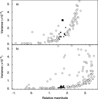
Figure 1.— Frame-to-frame photometric variances (in magnitudes) of all stars (gray circles and black crosses) in the $(35671)\,1998\,\rm{SN}_{165}$ (a) and $(38628)\,\rm{Huya}$ (b) fields, plotted against their relative magnitude. The trend of increasing photometric variability with increasing magnitude is clear. The intrinsically variable stars clearly do not follow this trend, and are located towards the upper left region of the plot. The KBOs are shown as black squares. $(35671)\,1998\,\rm{SN}_{165}$, in the top panel shows a much larger variability than the comparison stars (shown as crosses, see Section 3.1), while $(38628)\,\rm{Huya}$ is well within the expected variance range, given its magnitude.

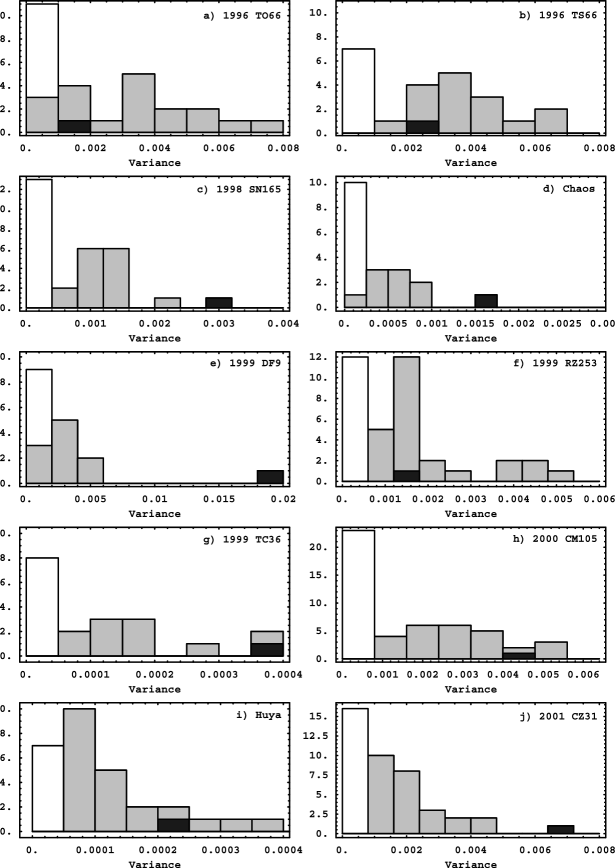
Figure 2.— Stacked histograms of the frame-to-frame variance (in magnitudes) in the optical data on the “reference” stars (in white), “comparison” stars (in gray), and the KBO (in black). In c), e), and j) the KBO shows significantly more variability than the comparison stars, whereas in all other cases it falls well within the range of photometric uncertainties of the stars of similar brightness.

Table 1Observing Conditions and Geometry

Object Designation		ObsDate	Tel.	Seeing	MvtRt	ITime	RA	dec	$R$	$\Delta$	$\alpha$
				[″]	[″/hr]	[sec]	[hhmmss]	[°′″]	[AU]	[AU]	[deg]
(19308)	$1996\,\rm{TO}_{66}$	99-Oct-01	WHT	1.8	2.89	500	23 59 46	+03 36 42	45.950	44.958	0.1594
	$1996\,\rm{TS}_{66}$	99-Sep-30	WHT	1.3	2.62	400,600	02 26 06	+21 41 03	38.778	37.957	0.8619
	$1996\,\rm{TS}_{66}$	99-Oct-01	WHT	1.1	2.67	600	02 26 02	+21 40 50	38.778	37.948	0.8436
	$1996\,\rm{TS}_{66}$	99-Oct-02	WHT	1.5	2.70	600,900	02 25 58	+21 40 35	38.778	37.939	0.8225
(35671)	$1998\,\rm{SN}_{165}$	99-Sep-29	WHT	1.5	3.24	360,400	23 32 46	$-$01 18 15	38.202	37.226	0.3341
(35671)	$1998\,\rm{SN}_{165}$	99-Sep-30	WHT	1.4	3.22	360	23 32 41	$-$01 18 47	38.202	37.230	0.3594
(19521)	Chaos	99-Oct-01	WHT	1.0	1.75	360,400,600	03 44 37	+21 30 58	42.399	41.766	1.0616
(19521)	Chaos	99-Oct-02	WHT	1.5	1.79	400,600	03 44 34	+21 30 54	42.399	41.755	1.0484
(79983)	$1999\,\rm{DF}_{9}$	01-Feb-13	WHT	1.7	3.19	900	10 27 04	+09 45 16	39.782	38.818	0.3124
(79983)	$1999\,\rm{DF}_{9}$	01-Feb-14	WHT	1.6	3.21	900	10 26 50	+09 46 25	39.783	38.808	0.2436
(79983)	$1999\,\rm{DF}_{9}$	01-Feb-15	WHT	1.4	3.22	900	10 26 46	+09 46 50	39.783	38.806	0.2183
(80806)	$2000\,\rm{CM}_{105}$	01-Feb-11	WHT	1.5	3.14	600,900	09 18 48	+19 41 59	41.753	40.774	0.1687
(80806)	$2000\,\rm{CM}_{105}$	01-Feb-13	WHT	1.4	3.12	900	09 18 39	+19 42 40	41.753	40.778	0.2084
(80806)	$2000\,\rm{CM}_{105}$	01-Feb-14	WHT	1.5	3.11	900	09 18 34	+19 43 02	41.753	40.781	0.2303
(66652)	$1999\,\rm{RZ}_{253}$	01-Sep-11	INT	1.9	2.86	600	22 02 57	$-$12 31 06	40.963	40.021	0.4959
(66652)	$1999\,\rm{RZ}_{253}$	01-Sep-12	INT	1.4	2.84	600	22 02 53	$-$12 31 26	40.963	40.026	0.5156
(66652)	$1999\,\rm{RZ}_{253}$	01-Sep-13	INT	1.8	2.82	600	22 02 49	$-$12 31 49	40.963	40.033	0.5381
(47171)	$1999\,\rm{TC}_{36}$	01-Sep-11	INT	1.9	3.85	600	00 16 49	$-$07 34 59	31.416	30.440	0.4605
(47171)	$1999\,\rm{TC}_{36}$	01-Sep-12	INT	1.4	3.86	900	00 16 45	$-$07 35 33	31.416	30.437	0.4359
(47171)	$1999\,\rm{TC}_{36}$	01-Sep-13	INT	1.8	3.88	900	00 16 39	$-$07 36 13	31.416	30.434	0.4122
(38628)	Huya	01-Feb-28	INT	1.5	2.91	600	13 31 13	$-$00 39 04	29.769	29.021	1.2725
(38628)	Huya	01-Mar-01	INT	1.8	2.97	360	13 31 09	$-$00 38 23	29.768	29.009	1.2479
(38628)	Huya	01-Mar-03	INT	1.5	3.08	360	13 31 01	$-$00 36 59	29.767	28.987	1.1976
	$2001\,\rm{CZ}_{31}$	01-Mar-01	INT	1.3	2.72	600,900	09 00 03	+16 29 23	41.394	40.522	0.6525
	$2001\,\rm{CZ}_{31}$	01-Mar-03	INT	1.4	2.65	600,900	08 59 54	+16 30 04	41.394	40.539	0.6954

Table 2Properties of Observed KBOs

Object Designation		Class	$H$	$i$	$e$	$a$
			[mag]	[deg]		[AU]
(19308)	$1996\,\rm{TO}_{66}$	C	4.5	27.50	0.12	43.20
	$1996\,\rm{TS}_{66}$	C	6.4	7.30	0.13	44.00
(35671)	$1998\,\rm{SN}_{165}$	C	5.8	4.60	0.05	37.80
(19521)	Chaos	C	4.9	12.00	0.11	45.90
(79983)	$1999\,\rm{DF}_{9}$	C	6.1	9.80	0.15	46.80
(80806)	$2000\,\rm{CM}_{105}$	C	6.2	3.80	0.07	42.50
(66652)	$1999\,\rm{RZ}_{253}$	C	5.9	0.60	0.09	43.60
(47171)	$1999\,\rm{TC}_{36}$	Pb	4.9	8.40	0.22	39.30
(38628)	Huya	P	4.7	15.50	0.28	39.50
	$2001\,\rm{CZ}_{31}$	C	5.4	10.20	0.12	45.60

We collected time-series optical data on 10 KBOs at the Isaac Newton 2.5m (INT) and William Herschel 4m (WHT) telescopes. The INT Wide Field Camera (WFC) is a mosaic of 4 EEV 2048$\times$4096 CCDs, each with a pixel scale of 0$\farcs$33/pixel and spanning approximately 11$\farcm$3$\times$22$\farcm$5 in the plane of the sky. The targets are imaged through a Johnson R filter. The WHT prime focus camera consists of 2 EEV 2048$\times$4096 CCDs with a pixel scale of 0$\farcs$24/pixel, and covers a sky-projected area of 2$\times$8$\farcm$2$\times$16$\farcm$4. With this camera we used a Harris R filter. The seeing for the whole set of observations ranged from 1.0 to 1.9″FWHM. We tracked both telescopes at sidereal rate and kept integration times for each object sufficiently short to avoid errors in the photometry due to trailing effects (see Table 1). No light travel time corrections have been made.

We reduced the data using standard techniques. The sky background in the flat-fielded images shows variations of less than 1% across the chip. Background variations between consecutive nights were less than 5% for most of the data. Cosmic rays were removed with the package LA-Cosmic (van Dokkum 2001).

We performed aperture photometry on all objects in the field using the SExtractor software package (Bertin & Arnouts 1996). This software performs circular aperture measurements on each object in a frame, and puts out a catalog of both the magnitudes and the associated errors. Below we describe how we obtained a better estimate of the errors. We used apertures ranging from 1.5 to 2.0 times the FWHM for each frame and selected the aperture that maximized signal-to-noise. An extra aperture of 5 FWHMs was used to look for possible seeing dependent trends in our photometry. The catalogs were matched by selecting only the sources that are present in all frames. The slow movement of KBOs from night to night allows us to successfully match a large number of sources in consecutive nights. We discarded all saturated sources as well as those identified to be galaxies.

The KBO lightcurves were obtained from differential photometry with respect to the brightest non-variable field stars. An average of the magnitudes of the brightest stars (the ”reference” stars) provides a reference for differential photometry in each frame. This method allows for small amplitude brightness variations to be detected even under non-photometric conditions.

The uncertainty in the relative photometry was calculated from the scatter in the photometry of field stars that are similar to the KBOs in brightness (the ”comparison” stars, see Fig.1). This error estimate is more robust than the errors provided by SExtractor (see below), and was used to verify the accuracy of the latter. This procedure resulted in consistent time series brightness data for $\sim 100$ objects (KBO + field stars) in a time span of 2–3 consecutive nights.

We observed Landolt standard stars whenever conditions were photometric, and used them to calibrate the zero point of the magnitude scale. The extinction coefficient was obtained from the reference stars.

Since not all nights were photometric the lightcurves are presented as variations with respect to the mean brightness. These yield the correct amplitudes and periods of the lightcurves but do not provide their absolute magnitudes.

The orbital parameters and other properties of the observed KBOs are given in Table 2. Tables 3, 4, 5, and 6 list the absolute $R$-magnitude photometric measurements obtained for $(19308)\,1996\,\rm{TO}_{66}$, $1996\,\rm{TS}_{66}$, $(35671)\,1998\,\rm{SN}_{165}$, and $(19521)\,\rm{Chaos}$, respectively. Tables 7 and 8 list the mean-subtracted $R$-band data for $(79983)\,1999\,\rm{DF}_{9}$ and $2001\,\rm{CZ}_{31}$.

Table 3Photometric measurements of $(19308)\,1996\,\rm{TO}_{66}$

		$m_{R}$
UT Date	Julian Date	[mag]
1999 Oct 1.84831	2451453.34831	21.24 $\pm$ 0.07
1999 Oct 1.85590	2451453.35590	21.30 $\pm$ 0.07
1999 Oct 1.86352	2451453.36352	21.20 $\pm$ 0.07
1999 Oct 1.87201	2451453.37201	21.22 $\pm$ 0.07
1999 Oct 1.87867	2451453.37867	21.21 $\pm$ 0.07
1999 Oct 1.88532	2451453.38532	21.28 $\pm$ 0.07
1999 Oct 1.89302	2451453.39302	21.27 $\pm$ 0.06
1999 Oct 1.90034	2451453.40034	21.30 $\pm$ 0.06
1999 Oct 1.90730	2451453.40730	21.28 $\pm$ 0.06
1999 Oct 1.91470	2451453.41470	21.31 $\pm$ 0.06

Table 4Photometric measurements of $1996\,\rm{TS}_{66}$

		$m_{R}$
UT Date	Julian Date	[mag]
1999 Sep 30.06087	2451451.56087	21.94 $\pm$ 0.07
1999 Sep 30.06628	2451451.56628	21.83 $\pm$ 0.07
1999 Sep 30.07979	2451451.57979	21.76 $\pm$ 0.07
1999 Sep 30.08529	2451451.58529	21.71 $\pm$ 0.07
1999 Sep 30.09068	2451451.59068	21.75 $\pm$ 0.07
1999 Sep 30.09695	2451451.59695	21.67 $\pm$ 0.07
1999 Sep 30.01250	2451451.60250	21.77 $\pm$ 0.07
1999 Sep 30.10936	2451451.60936	21.76 $\pm$ 0.06
1999 Sep 30.11705	2451451.61705	21.80 $\pm$ 0.06
1999 Sep 30.12486	2451451.62486	21.77 $\pm$ 0.06
1999 Sep 30.13798	2451451.63798	21.82 $\pm$ 0.07
1999 Sep 30.14722	2451451.64722	21.74 $\pm$ 0.06
1999 Sep 30.15524	2451451.65524	21.72 $\pm$ 0.06
1999 Sep 30.16834	2451451.66834	21.72 $\pm$ 0.08
1999 Sep 30.17680	2451451.67680	21.83 $\pm$ 0.07
1999 Sep 30.18548	2451451.68548	21.80 $\pm$ 0.06
1999 Sep 30.19429	2451451.69429	21.74 $\pm$ 0.07
1999 Sep 30.20212	2451451.70212	21.78 $\pm$ 0.07
1999 Sep 30.21010	2451451.71010	21.72 $\pm$ 0.07
1999 Sep 30.21806	2451451.71806	21.76 $\pm$ 0.09
1999 Sep 30.23528	2451451.73528	21.73 $\pm$ 0.07
1999 Sep 30.24355	2451451.74355	21.74 $\pm$ 0.08
1999 Oct 01.02002	2451452.52002	21.81 $\pm$ 0.06
1999 Oct 01.02799	2451452.52799	21.82 $\pm$ 0.06
1999 Oct 01.03648	2451452.53648	21.81 $\pm$ 0.06
1999 Oct 01.04422	2451452.54422	21.80 $\pm$ 0.06
1999 Oct 01.93113	2451453.43113	21.71 $\pm$ 0.06
1999 Oct 01.94168	2451453.44168	21.68 $\pm$ 0.06
1999 Oct 01.95331	2451453.45331	21.73 $\pm$ 0.06
1999 Oct 01.97903	2451453.47903	21.69 $\pm$ 0.06
1999 Oct 01.99177	2451453.49177	21.74 $\pm$ 0.06
1999 Oct 02.00393	2451453.50393	21.73 $\pm$ 0.05
1999 Oct 02.01588	2451453.51588	21.78 $\pm$ 0.05
1999 Oct 02.02734	2451453.52734	21.71 $\pm$ 0.05

Table 5Photometric measurements of $(35671)\,1998\,\rm{SN}_{165}$

		$m_{R}$
UT Date	Julian Date	[mag]
1999 Sep 29.87384	2451451.37384	21.20 $\pm$ 0.06
1999 Sep 29.88050	2451451.38050	21.19 $\pm$ 0.05
1999 Sep 29.88845	2451451.38845	21.18 $\pm$ 0.05
1999 Sep 29.89811	2451451.39811	21.17 $\pm$ 0.05
1999 Sep 29.90496	2451451.40496	21.21 $\pm$ 0.05
1999 Sep 29.91060	2451451.41060	21.24 $\pm$ 0.05
1999 Sep 29.91608	2451451.41608	21.18 $\pm$ 0.05
1999 Sep 29.92439	2451451.42439	21.25 $\pm$ 0.05
1999 Sep 29.93055	2451451.43055	21.24 $\pm$ 0.05
1999 Sep 29.93712	2451451.43712	21.26 $\pm$ 0.06
1999 Sep 29.94283	2451451.44283	21.25 $\pm$ 0.06
1999 Sep 29.94821	2451451.44821	21.28 $\pm$ 0.06
1999 Sep 29.96009	2451451.46009	21.25 $\pm$ 0.06
1999 Sep 29.96640	2451451.46640	21.21 $\pm$ 0.06
1999 Sep 29.97313	2451451.47313	21.17 $\pm$ 0.05
1999 Sep 29.97850	2451451.47850	21.14 $\pm$ 0.05
1999 Sep 29.98373	2451451.48373	21.12 $\pm$ 0.06
1999 Sep 29.98897	2451451.48897	21.15 $\pm$ 0.06
1999 Sep 29.99469	2451451.49469	21.15 $\pm$ 0.06
1999 Sep 29.99997	2451451.49997	21.16 $\pm$ 0.06
1999 Sep 30.00521	2451451.50521	21.12 $\pm$ 0.06
1999 Sep 30.01144	2451451.51144	21.09 $\pm$ 0.06
1999 Sep 30.02164	2451451.52164	21.18 $\pm$ 0.06
1999 Sep 30.02692	2451451.52692	21.17 $\pm$ 0.06
1999 Sep 30.84539	2451452.34539	21.32 $\pm$ 0.06
1999 Sep 30.85033	2451452.35033	21.30 $\pm$ 0.06
1999 Sep 30.85531	2451452.35531	21.28 $\pm$ 0.06
1999 Sep 30.86029	2451452.36029	21.31 $\pm$ 0.06
1999 Sep 30.86550	2451452.36550	21.21 $\pm$ 0.06
1999 Sep 30.87098	2451452.37098	21.26 $\pm$ 0.06
1999 Sep 30.87627	2451452.37627	21.28 $\pm$ 0.06
1999 Sep 30.89202	2451452.39202	21.23 $\pm$ 0.05
1999 Sep 30.89698	2451452.39698	21.30 $\pm$ 0.06
1999 Sep 30.90608	2451452.40608	21.20 $\pm$ 0.05
1999 Sep 30.91191	2451452.41191	21.26 $\pm$ 0.05
1999 Sep 30.92029	2451452.42029	21.15 $\pm$ 0.05
1999 Sep 30.92601	2451452.42601	21.19 $\pm$ 0.05
1999 Sep 30.93110	2451452.43110	21.14 $\pm$ 0.05
1999 Sep 30.93627	2451452.43627	21.16 $\pm$ 0.05
1999 Sep 30.94858	2451452.44858	21.18 $\pm$ 0.05
1999 Sep 30.95363	2451452.45363	21.16 $\pm$ 0.05
1999 Sep 30.95852	2451452.45852	21.13 $\pm$ 0.05
1999 Sep 30.96347	2451452.46347	21.17 $\pm$ 0.05
1999 Sep 30.96850	2451452.46850	21.16 $\pm$ 0.05
1999 Sep 30.97422	2451452.47422	21.18 $\pm$ 0.05
1999 Sep 30.98431	2451452.48431	21.18 $\pm$ 0.05
1999 Sep 30.98923	2451452.48923	21.17 $\pm$ 0.06
1999 Sep 30.99444	2451452.49444	21.16 $\pm$ 0.05
1999 Sep 30.99934	2451452.49934	21.20 $\pm$ 0.05
1999 Oct 01.00424	2451452.50424	21.16 $\pm$ 0.05
1999 Oct 01.00992	2451452.50992	21.18 $\pm$ 0.06

Table 6Photometric measurements of (19521) Chaos

		$m_{R}$
UT Date	Julian Date	[mag]
1999 Oct 01.06329	2451452.56329	20.82 $\pm$ 0.06
1999 Oct 01.06831	2451452.56831	20.80 $\pm$ 0.06
1999 Oct 01.07324	2451452.57324	20.80 $\pm$ 0.06
1999 Oct 01.07817	2451452.57817	20.81 $\pm$ 0.06
1999 Oct 01.08311	2451452.58311	20.80 $\pm$ 0.06
1999 Oct 01.08801	2451452.58801	20.76 $\pm$ 0.06
1999 Oct 01.09370	2451452.59370	20.77 $\pm$ 0.06
1999 Oct 01.14333	2451452.64333	20.71 $\pm$ 0.06
1999 Oct 01.15073	2451452.65073	20.68 $\pm$ 0.06
1999 Oct 01.15755	2451452.65755	20.70 $\pm$ 0.06
1999 Oct 01.16543	2451452.66543	20.72 $\pm$ 0.06
1999 Oct 01.17316	2451452.67316	20.72 $\pm$ 0.06
1999 Oct 01.18112	2451452.68112	20.71 $\pm$ 0.06
1999 Oct 01.18882	2451452.68882	20.73 $\pm$ 0.06
1999 Oct 01.19652	2451452.69652	20.70 $\pm$ 0.06
1999 Oct 01.20436	2451452.70436	20.69 $\pm$ 0.06
1999 Oct 01.21326	2451452.71326	20.72 $\pm$ 0.06
1999 Oct 01.21865	2451452.71865	20.72 $\pm$ 0.06
1999 Oct 01.22402	2451452.72402	20.74 $\pm$ 0.06
1999 Oct 01.22938	2451452.72938	20.72 $\pm$ 0.06
1999 Oct 01.23478	2451452.73478	20.71 $\pm$ 0.07
1999 Oct 01.24022	2451452.74022	20.72 $\pm$ 0.07
1999 Oct 02.04310	2451453.54310	20.68 $\pm$ 0.06
1999 Oct 02.04942	2451453.54942	20.69 $\pm$ 0.06
1999 Oct 02.07568	2451453.57568	20.74 $\pm$ 0.07
1999 Oct 02.08266	2451453.58266	20.73 $\pm$ 0.06
1999 Oct 02.09188	2451453.59188	20.74 $\pm$ 0.06
1999 Oct 02.10484	2451453.60484	20.75 $\pm$ 0.06
1999 Oct 02.11386	2451453.61386	20.77 $\pm$ 0.06
1999 Oct 02.12215	2451453.62215	20.77 $\pm$ 0.06
1999 Oct 02.13063	2451453.63063	20.78 $\pm$ 0.06
1999 Oct 02.13982	2451453.63982	20.79 $\pm$ 0.06
1999 Oct 02.14929	2451453.64929	20.71 $\pm$ 0.07

Table 7Relative photometry measurements of $(79983)\,1999\,\rm{DF}_{9}$

		$\delta m_{R}$
UT Date	Julian Date	[mag]
2001 Feb 13.13417	2451953.63417	0.21 $\pm$ 0.02
2001 Feb 13.14536	2451953.64536	0.20 $\pm$ 0.03
2001 Feb 13.15720	2451953.65720	0.17 $\pm$ 0.04
2001 Feb 13.16842	2451953.66842	0.06 $\pm$ 0.03
2001 Feb 13.17967	2451953.67967	-0.08 $\pm$ 0.02
2001 Feb 13.20209	2451953.70209	-0.09 $\pm$ 0.03
2001 Feb 13.21325	2451953.71325	-0.05 $\pm$ 0.03
2001 Feb 13.22439	2451953.72439	-0.15 $\pm$ 0.03
2001 Feb 13.23554	2451953.73554	-0.19 $\pm$ 0.04
2001 Feb 13.24671	2451953.74671	0.00 $\pm$ 0.04
2001 Feb 14.13972	2451954.63972	-0.05 $\pm$ 0.02
2001 Feb 14.15104	2451954.65104	-0.12 $\pm$ 0.02
2001 Feb 14.16228	2451954.66228	-0.25 $\pm$ 0.02
2001 Feb 14.17347	2451954.67347	-0.18 $\pm$ 0.02
2001 Feb 14.18477	2451954.68477	-0.14 $\pm$ 0.03
2001 Feb 14.19600	2451954.69600	-0.05 $\pm$ 0.03
2001 Feb 14.20725	2451954.70725	0.00 $\pm$ 0.03
2001 Feb 14.21860	2451954.71860	0.03 $\pm$ 0.03
2001 Feb 14.22987	2451954.72987	0.11 $\pm$ 0.04
2001 Feb 14.24112	2451954.74112	0.21 $\pm$ 0.04
2001 Feb 14.25234	2451954.75234	0.20 $\pm$ 0.05
2001 Feb 14.26356	2451954.76356	0.16 $\pm$ 0.05
2001 Feb 15.14518	2451955.64518	-0.06 $\pm$ 0.05
2001 Feb 15.15707	2451955.65707	-0.08 $\pm$ 0.02
2001 Feb 15.16831	2451955.66831	-0.15 $\pm$ 0.05
2001 Feb 15.19086	2451955.69086	0.05 $\pm$ 0.06
2001 Feb 15.20234	2451955.70234	0.19 $\pm$ 0.07
2001 Feb 15.23127	2451955.73127	0.04 $\pm$ 0.05

Table 8Relative photometry measurements of $2001\,\rm{CZ}_{31}$

		$\delta m_{R}$
UT Date	Julian Date	[mag]
2001 Feb 28.92789	2451969.42789	0.03 $\pm$ 0.05
2001 Feb 28.93900	2451969.43900	0.06 $\pm$ 0.04
2001 Feb 28.95013	2451969.45013	0.03 $\pm$ 0.04
2001 Feb 28.96120	2451969.46120	-0.09 $\pm$ 0.04
2001 Feb 28.97235	2451969.47235	-0.10 $\pm$ 0.04
2001 Feb 28.98349	2451969.48349	-0.12 $\pm$ 0.04
2001 Feb 28.99475	2451969.49475	-0.14 $\pm$ 0.03
2001 Mar 01.00706	2451969.50706	-0.02 $\pm$ 0.03
2001 Mar 01.01817	2451969.51817	0.00 $\pm$ 0.03
2001 Mar 01.02933	2451969.52933	0.03 $\pm$ 0.03
2001 Mar 01.04046	2451969.54046	0.07 $\pm$ 0.04
2001 Mar 01.05153	2451969.55153	0.10 $\pm$ 0.04
2001 Mar 01.06304	2451969.56304	0.06 $\pm$ 0.04
2001 Mar 01.08608	2451969.58608	-0.05 $\pm$ 0.04
2001 Mar 01.09808	2451969.59808	-0.05 $\pm$ 0.05
2001 Mar 03.01239	2451971.51239	0.15 $\pm$ 0.05
2001 Mar 03.02455	2451971.52455	-0.01 $\pm$ 0.05
2001 Mar 03.03596	2451971.53596	0.00 $\pm$ 0.04
2001 Mar 03.04731	2451971.54731	-0.02 $\pm$ 0.03
2001 Mar 03.05865	2451971.55865	-0.08 $\pm$ 0.04
2001 Mar 03.07060	2451971.57060	-0.04 $\pm$ 0.04
2001 Mar 03.08212	2451971.58212	0.01 $\pm$ 0.03

3. Lightcurve Analysis

The results in this paper depend solely on the amplitude and period of the KBO lightcurves. It is therefore important to accurately determine these parameters and the associated uncertainties.

3.1. Can we detect the KBO brightness variation?

We begin by investigating if the observed brightness variations are intrinsic to the KBO, i.e., if the KBO’s intrinsic brightness variations are detectable given our uncertainties. This was done by comparing the frame-to-frame scatter in the KBO optical data with that of ($\sim 10-20$) comparison stars.

To visually compare the scatter in the magnitudes of the reference stars (see Section 2), comparison stars, and KBOs, we plot a histogram of their frame-to-frame variances (see Fig. 2). In general such a histogram should show the reference stars clustered at the lowest variances, followed by the comparison stars spread over larger variances. If the KBO appears isolated at much higher variances than both groups of stars (e.g., Fig. 2j), then its brightness modulations are significant. Conversely, if the KBO is clustered with the stars (e.g. Fig. 2f), any periodic brightness variations would be below the detection threshold.

Figure 1 shows the dependence of the uncertainties on magnitude. Objects that do not fall on the rising curve traced out by the stars must have intrinsic brightness variations. By calculating the mean and spread of the variance for the comparison stars (shown as crosses) we can calculate our photometric uncertainties and thus determine whether the KBO brightness variations are significant ($\geq$3$\sigma$).

3.2. Period determination

In the cases where significant brightness variations (see Section 3.1) were detected in the lightcurves, the phase dispersion minimization method was used (PDM, Stellingwerf 1978) to look for periodicities in the data. For each test period, PDM computes a statistical parameter $\theta$ that compares the spread of data points in phase bins with the overall spread of the data. The period that best fits the data is the one that minimizes $\theta$. The advantages of PDM are that it is non-parametric, i.e., it does not assume a shape for the lightcurve, and it can handle unevenly spaced data. Each data set was tested for periods ranging from 2 to 24 hours, in steps of 0.01 hr. To assess the uniqueness of the PDM solution, we generated 100 Monte Carlo realizations of each lightcurve, keeping the original data times and randomizing the magnitudes within the error bars. We ran PDM on each generated dataset to obtain a distribution of best-fit periods.

Table 9Lightcurve Properties of Observed KBOs

Object Designation		$m_{R}$	Nts	$\Delta m_{R}$	$P$
		[mag]		[mag]	[hr]
(35671)	$1998\,\rm{SN}_{165}$	21.20$\pm$0.05	2(1)	0.16$\pm$0.01	8.84 (8.70)
(79983)	$1999\,\rm{DF}_{9}$	–	3	0.40$\pm$0.02	6.65 (9.00)
	$2001\,\rm{CZ}_{31}$		2(1)	0.21$\pm$0.02	4.71 (5.23)
(19308)	$1996\,\rm{TO}_{66}$	21.26$\pm$0.06	1	?
	$1996\,\rm{TS}_{66}$	21.76$\pm$0.05	3	$<$0.15
(19521)	Chaos	20.74$\pm$0.06	2	$<$0.10
(80806)	$2000\,\rm{CM}_{105}$	–	2	$<$0.14
(66652)	$1999\,\rm{RZ}_{253}$	–	3	$<$0.05
(47171)	$1999\,\rm{TC}_{36}$	–	3	$<$0.07
(38628)	Huya	–	2	$<$0.04

3.3. Amplitude determination

We used a Monte Carlo experiment to determine the amplitude of the lightcurves for which a period was found. We generated several artificial data sets by randomizing each point within the error bar. Each artificial data set was fitted with a Fourier series, using the best-fit period, and the mode and central 68% of the distribution of amplitudes were taken as the lightcurve amplitude and $1\sigma$ uncertainty, respectively.

For the null lightcurves, i.e. those where no significant variation was detected, we subtracted the typical error bar size from the total amplitude of the data to obtain an upper limit to the amplitude of the KBO photometric variation.

4. Results

In this section we present the results of the lightcurve analysis for each of the observed KBOs. We found significant brightness variations ($\Delta m>0.15\,$mag) for 3 out of 10 KBOs (30%), and $\Delta m\geq 0.40\,$mag for 1 out of 10 (10%). This is consistent with previously published results: Sheppard & Jewitt (2002, hereafter SJ02) found a fraction of 31% with $\Delta m>0.15\,$mag and 23% with $\Delta m>0.40\,$mag, both consistent with our results. The other 7 KBOs do not show detectable variations. The results are summarized in Table 9.

4.1. 1998 SN₁₆₅

Figure 3.— Periodogram for the data on $(35671)\,1998\,\rm{SN}_{165}$. The lower left panel (b) shows an enlarged section near the minimum calculated using only the data published in this paper, and the lower right panel (c) shows the same region recalculated after adding the PDR02 data.

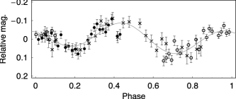
Figure 4.— Lightcurve of $(35671)\,1998\,\rm{SN}_{165}$. The figure represents the data phased with the best fit period $P=8.84\,$hr. Different symbols correspond to different nights of observation. The gray line is a 2nd order Fourier series fit to the data. The PDR02 data are shown as crosses.

The brightness of $(35671)\,1998\,\rm{SN}_{165}$ varies significantly ($>5\sigma$) more than that of the comparison stars (see Figs. 1 and 2c). The periodogram for this KBO shows a very broad minimum around $P=9\,$hr (Fig. 3a). The degeneracy implied by the broad minimum would only be resolved with additional data. A slight weaker minimum is seen at $P=6.5\,$hr, which is close to a 24 hr alias of $P=9\,$hr.

Peixinho et al. (2002, hereafter PDR02) observed this object in September 2000, but having only one night’s worth of data, they did not succeed in determining this object’s rotational period unambiguously. We used their data to solve the degeneracy in our PDM result. The PDR02 data have not been absolutely calibrated, and the magnitudes are given relative to a bright field star. To be able to combine it with our own data we had to subtract the mean magnitudes. Our periodogram of $(35671)\,1998\,\rm{SN}_{165}$ (centered on the broad minimum) is shown in Fig. 3b and can be compared with the revised periodogram obtained with our data combined with the PDR02 data (Fig. 3c). The minima become much clearer with the additional data, but because of the 1-year time difference between the two observational campaigns, many close aliases appear in the periodogram. The absolute minimum, at $P=8.84\,$hr, corresponds to a double peaked lightcurve (see Fig. 4). The second best fit, $P=8.7\,$hr, produces a more scattered phase plot, in which the peak in the PDR02 data coincides with our night 2. Period $P=8.84\,$hr was also favored by the Monte Carlo method described in Section 3.2, being identified as the best fit in 55% of the cases versus 35% for $P=8.7\,$hr. The large size of the error bars compared to the amplitude is responsible for the ambiguity in the result. We will use $P=8.84\,$hr in the rest of the paper because it was consistently selected as the best fit.

The amplitude, obtained using the Monte Carlo method described in Section 3.3, is $\Delta m=0.16\pm 0.01\,$mag. This value was calculated using only our data, but it did not change when recalculated adding the PDR02 data.

4.2. 1999 DF₉

Figure 5.— Periodogram for the $(79983)\,1999\,\rm{DF}_{9}$ data. The minimum corresponds to a lightcurve period $P=6.65\,$hr.

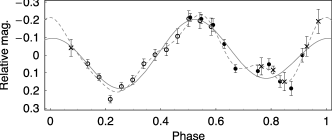
Figure 6.— Same as Fig. 4 for KBO $(79983)\,1999\,\rm{DF}_{9}$. The best fit period is $P=6.65\,$hr. The lines represent a 2nd order (solid line) and 5th (dashed line) order Fourier series fits to the data. Normalized $\chi^{2}$ values of the fits are 2.8 and 1.3 respectively.

$(79983)\,1999\,\rm{DF}_{9}$ shows large amplitude photometric variations ($\Delta m_{R}\sim 0.4\,$mag). The PDM periodogram for $(79983)\,1999\,\rm{DF}_{9}$ is shown in Fig. 5. The best-fit period is $P=6.65\,$hr, which corresponds to a double-peak lightcurve (Fig. 6). Other PDM minima are found close to $P/2\approx 3.3\,$hr and $9.2\,$hr, a $24\,$hr alias of the best period. Phasing the data with $P/2$ results in a worse fit because the two minima of the double peaked lightcurve exhibit significantly different morphologies (Fig. 6); the peculiar sharp feature superimposed on the brighter minimum, which is reproduced on two different nights, may be caused by a non-convex feature on the surface of the KBO (Torppa et al. 2003). Period $P=6.65\,$hr was selected in 65 of the 100 Monte Carlo replications of the dataset (see Section 3.2). The second most selected solution (15%) was at $P=9\,$hr. We will use $P=6.65\,$hr for the rest of the paper.

The amplitude of the lightcurve, estimated as described in Section 3.3, is $\Delta m_{R}=0.40\pm 0.02\,$mag.

4.3. 2001 CZ₃₁

Figure 7.— Periodogram for the $2001\,\rm{CZ}_{31}$ data. The lower left panel (b) shows an enlarged section near the minimum calculated using only the data published in this paper, and the lower right panel (c) shows the same region recalculated after adding the SJ02 data.

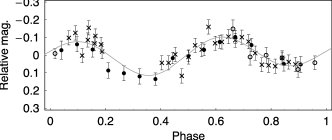
Figure 8.— Same as Fig. 4 for KBO $2001\,\rm{CZ}_{31}$. The data are phased with period $P=4.71\,$hr. The points represented by crosses are taken from SJ02.

This object shows substantial brightness variations ($4.5\sigma$ above the comparison stars) in a systematic manner. The first night of data seems to sample nearly one complete rotational phase. As for $(35671)\,1998\,\rm{SN}_{165}$, the $2001\,\rm{CZ}_{31}$ data span only two nights of observations. In this case, however, the PDM minima (see Figs. 7a and 7b) are very narrow and only two correspond to independent periods, $P=4.69\,$hr (the minimum at $5.82\,$ is a $24\,$hr alias of $4.69\,$hr), and $P=5.23\,$hr.

$2001\,\rm{CZ}_{31}$ has also been observed by SJ02 in February and April 2001, with inconclusive results. We used their data to try to rule out one (or both) of the two periods we found. We mean-subtracted the SJ02 data in order to combine it with our uncalibrated observations. Figure 7c shows the section of the periodogram around $P=5\,$hr, recalculated using SJ02’s first night plus our own data. The aliases are due to the 1 month time difference between the two observing runs. The new PDM minimum is at $P=4.71\,$hr – very close to the $P=4.69\,$hr determined from our data alone.

Visual inspection of the combined data set phased with $P=4.71\,$hr shows a very good match between SJ02’s first night (2001 Feb 20) and our own data (see Fig. 8). SJ02’s second and third nights show very large scatter and were not included in our analysis. Phasing the data with $P=5.23\,$hr yields a more scattered lightcurve, which confirms the PDM result. The Monte Carlo test for uniqueness yielded $P=4.71\,$hr as the best-fit period in 57% of the cases, followed by $P=5.23\,$hr in 21%, and a few other solutions, all below 10%, between $P=5\,$hr and $P=6\,$hr. We will use $P=4.71\,$hr throughout the rest of the paper.

We measured a lightcurve amplitude of $\Delta m=0.21\pm 0.02\,$mag. If we use both ours and SJ02’s first night data, $\Delta m$ rises to 0.22 mag.

4.4. Flat Lightcurves

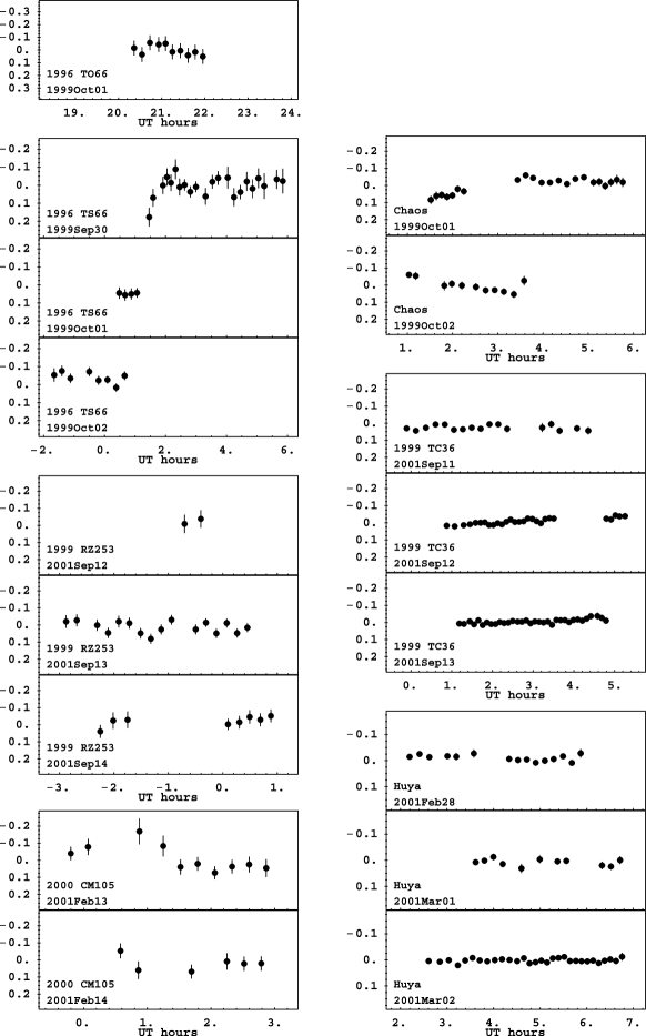
Figure 9.— The “flat” lightcurves are shown. The respective amplitudes are within the photometric uncertainties.

The fluctuations detected in the optical data on KBOs $(19308)\,1996\,\rm{TO}_{66}$, $1996\,\rm{TS}_{66}$, $(47171)\,1999\,\rm{TC}_{36}$, $(66652)\,1999\,\rm{RZ}_{253}$, $(80806)\,2000\,\rm{CM}_{105}$, and $(38628)\,\rm{Huya}$, are well within the uncertainties. $(19521)\,\rm{Chaos}$ shows some variations with respect to the comparison stars but no period was found to fit all the data. See Table 9 and Fig. 9 for a summary of the results.

4.5. Other lightcurve measurements

The KBO lightcurve database has increased considerably in the last few years, largely due to the observational campaign of SJ02, with recent updates in Sheppard & Jewitt (2003) and Sheppard & Jewitt (2004). These authors have published observations and rotational data for a total of 30 KBOs (their SJ02 paper includes data for 3 other previously published lightcurves in the analysis). Other recently published KBO lightcurves include those for $(50000)\,$Quaoar (Ortiz et al. 2003) and the scattered KBO $(29981)\,1999\,\rm{TD}_{10}$ (Rousselot et al. 2003). Of the 10 KBO lightcurves presented in this paper, 6 are new to the database, bringing the total to 41.

Table 4.5 lists the rotational data on the 41 KBOs that will be analyzed in the rest of the paper.

Table 10Database of KBOs Lightcurve Properties

Object Designation		Class	Size	$P$		$\Delta m_{R}$	Ref.
			[km]	[hr]		[mag]
KBOs considered to have $\Delta m<0.15\,$mag
(15789)	$1993\,\rm{SC}$	P	240			0.04	7, 2
(15820)	$1994\,\rm{TB}$	P	220			$<$0.04	10
(26181)	$1996\,\rm{GQ}_{21}$	S	730			$<$0.10	10
(15874)	$1996\,\rm{TL}_{66}$	S	480			0.06	7, 4
(15875)	$1996\,\rm{TP}_{66}$	P	250			0.12	7, 1
(79360)	$1997\,\rm{CS}_{29}$	C	630			$<$0.08	10
(91133)	$1998\,\rm{HK}_{151}$	P	170			$<$0.15	10
(33340)	$1998\,\rm{VG}_{44}$	P	280			$<$0.10	10
(19521)	Chaos	C	600			$<$0.10	13, 10
(26375)	$1999\,\rm{DE}_{9}$	S	700			$<$0.10	10
(47171)	$1999\,\rm{TC}_{36}$	Pb	300			$<$0.07	13, 11
(38628)	Huya	P	550			$<$0.04	13, 11
(82075)	$2000\,\rm{YW}_{134}$	S	790			$<$0.10	11
(82158)	$2001\,\rm{FP}_{185}$	S	400			$<$0.10	11
(82155)	$2001\,\rm{FZ}_{173}$	S	430			$<$0.06	10
	$2001\,\rm{KD}_{77}$	P	430			$<$0.10	11
(28978)	Ixion	P	820			$<$0.10	11, 5
	$2001\,\rm{QF}_{298}$	P	580			$<$0.10	11
(42301)	$2001\,\rm{UR}_{163}$	S	1020			$<$0.10	11
(42355)	$2002\,\rm{CR}_{46}$	S	210			$<$0.10	11
(55636)	$2002\,\rm{TX}_{300}$	C	710	16.	24	0.08$\pm$0.02	11
(55637)	$2002\,\rm{UX}_{25}$	C	1090			$<$0.10	11
(55638)	$2002\,\rm{VE}_{95}$	P	500			$<$0.10	11
(80806)	$2000\,\rm{CM}_{105}$	C	330			$<$0.14	13
(66652)	$1999\,\rm{RZ}_{253}$	Cb	170			$<$0.05	13
	$1996\,\rm{TS}_{66}$	C	300			$<$0.14	13
KBOs considered to have $\Delta m\geq 0.15\,$mag
(32929)	$1995\,\rm{QY}_{9}$	P	180	7.	3	0.60$\pm$0.04	10, 7
(24835)	$1995\,\rm{SM}_{55}$	C	630	8.	08	0.19$\pm$0.05	11
(19308)	$1996\,\rm{TO}_{66}$	C	720	7.	9	0.26$\pm$0.03	11, 3
(26308)	$1998\,\rm{SM}_{165}$	R	240	7.	1	0.45$\pm$0.03	10, 8
(33128)	$1998\,\rm{BU}_{48}$	S	210	9.	8	0.68$\pm$0.04	10, 8
(40314)	$1999\,\rm{KR}_{16}$	C	400	11.	858	0.18$\pm$0.04	10
(47932)	$2000\,\rm{GN}_{171}$	P	360	8.	329	0.61$\pm$0.03	10
(20000)	Varuna	C	980	6.	34	0.42$\pm$0.03	10
	$2003\,\rm{AZ}_{84}$	P	900	13.	44	0.14$\pm$0.03	11
	$2001\,\rm{QG}_{298}$	Pcb	240	13.	7744	1.14$\pm$0.04	12
(50000)	Quaoar	C	1300	17.	6788	0.17$\pm$0.02	6
(29981)	$1999\,\rm{TD}_{10}$	S	100	15.	3833	0.53$\pm$0.03	9
(35671)	$1998\,\rm{SN}_{165}$	C	400	8.	84	0.16$\pm$0.01	13
(79983)	$1999\,\rm{DF}_{9}$	C	340	6.	65	0.40$\pm$0.02	13
	$2001\,\rm{CZ}_{31}$	C	440	4.	71	0.21$\pm$0.06	13

References. — (1) Collander-Brown et al. (1999); (2) Davies et al. (1997); (3) Hainaut et al. (2000); (4) Luu & Jewitt (1998); (5) Ortiz et al. (2001); (6) Ortiz et al. (2003); (7) Romanishin & Tegler (1999); (8) Romanishin et al. (2001); (9) Rousselot et al. (2003); (10) Sheppard & Jewitt (2002); (11) Sheppard & Jewitt (2003); (12) Sheppard & Jewitt (2004); (13) this work.

5. Analysis

In this section we examine the lightcurve properties of KBOs and compare them with those of main-belt asteroids (MBAs). The lightcurve data for these two families of objects cover different size ranges. MBAs, being closer to Earth, can be observed down to much smaller sizes than KBOs; in general it is very difficult to obtain good quality lightcurves for KBOs with diameters $D<50\,$km. Furthermore, some KBOs surpass the $1000\,$km barrier whereas the largest asteroid, Ceres, does not reach $900\,$km. This will be taken into account in the analysis.

The lightcurve data for asteroids were taken from the Harris Lightcurve Catalog, Version 5, while the diameter data were obtained from the Lowell Observatory database of asteroids orbital elements. The sizes of most KBOs were calculated from their absolute magnitude assuming an albedo of 0.04. The exceptions are (47171) 1999 TC₃₆, (38638) Huya, (28978) Ixion, (55636) 2002 TX₃₆, (66652) 1999 RZ₃₆, (26308) 1998 SM₁₆₅, and (20000) Varuna for which the albedo has been shown to be inconsistent with the value 0.04 (Grundy et al. 2005). For example, in the case of (20000) Varuna simultaneous thermal and optical observations have yielded a red geometric albedo of 0.070${}_{-0.017}^{+0.030}$ (Jewitt et al. 2001).

5.1. Spin period statistics

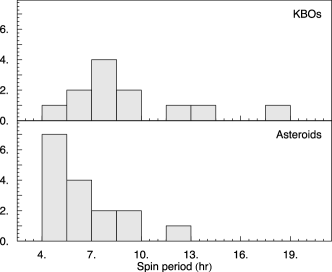
Figure 10.— Histograms of the spin periods of KBOs (upper panel) and main belt asteroids (lower panel) satisfying $D>200\,$km, $\Delta m\geq 0.15\,$mag, $P<20\,$hr. The mean rotational periods of KBOs and MBAs are 9.23 hr and 6.48 hr, respectively. The $y$-axis in both cases indicates the number of objects in each range of spin periods.

As Fig. 10 shows, the spin period distributions of KBOs and MBAs are significantly different. Because the sample of KBOs of small size or large periods is poor, to avoid bias in our comparison we consider only KBOs and MBAs with diameter larger than $200\,$km and with periods below $20\,$hr. In this range the mean rotational periods of KBOs and MBAs are $9.23\,$hr and $6.48\,$hr, respectively, and the two are different with a 98.5% confidence according to Student’s $t$-test. However, the different means do not rule that the underlying distributions are the same, and could simply mean that the two sets of data sample the same distribution differently. This is not the case, however, according to the Kolmogorov-Smirnov (K-S) test, which gives a probability that the periods of KBOs and MBAs are drawn from the same parent distribution of 0.7%.

Although it is clear that KBOs spin slower than asteroids, it is not clear why this is so. If collisions have contributed as significantly to the angular momentum of KBOs as they did for MBAs (Farinella et al. 1982, Catullo et al. 1984), then the observed difference should be related to how these two families react to collision events. We will address the question of the collisional evolution of KBO spin rates in a future paper.

5.2. Lightcurve amplitudes and the shapes of KBOs

Figure 11.— Cumulative distribution of lightcurve amplitude for KBOs (circles) and asteroids (crosses) larger than $200\,$km. We plot only KBOs for which a period has been determined. KBO 2001$\,QG_{298}$, thought to be a contact binary (Sheppard & Jewitt 2004), is not plotted although it may be considered an extreme case of elongation.

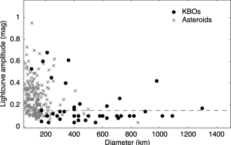
Figure 12.— Lightcurve amplitudes of KBOs (black circles) and main belt asteroids (gray crosses) plotted against object size.

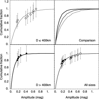
Figure 13.— Observed cumulative lightcurve amplitude distributions of KBOs (black circles) with diameter smaller than $400\,$km (upper left panel), larger than $400\,$km (lower left panel), and of all the sample (lower right panel) are shown as black circles. Error bars are Poissonian. The best fit power-law shape distributions of the form $f(\tilde{a})\,{\rm d}\tilde{a}=\tilde{a}^{-q}\,{\rm d}\tilde{a}$ were converted to amplitude distributions using a Monte Carlo technique (see text for details), and are shown as solid lines. The best fit $q$’s are listed in Table 11.

The cumulative distribution of KBO lightcurve amplitudes is shown in Fig. 11. It rises very steeply in the low amplitude range ($\Delta m<0.15\,$mag), and then becomes shallower reaching large amplitudes. In quantitative terms, $\sim 70\%$ of the KBOs possess $\Delta m<0.15\,$mag, while $\sim 12\%$ possess $\Delta m\geq 0.40\,$mag, with the maximum value being $\Delta m=0.68\,$mag. [Note: Fig. 11 does not include the KBO 2001 QG₂₉₈ which has a lightcurve amplitude $\Delta m=1.14\pm 0.04\,$mag, and would further extend the range of amplitudes. We do not include 2001 QG₂₉₈ in our analysis because it is thought to be a contact binary (Sheppard & Jewitt 2004)]. Figure 11 also compares the KBO distribution with that of MBAs. The distributions of the two populations are clearly distinct: there is a larger fraction of KBOs in the low amplitude range ($\Delta m<0.15\,$mag) than in the case of MBAs, and the KBO distribution extends to larger values of $\Delta m$.

Figure 12 shows the lightcurve amplitude of KBOs and MBAs plotted against size. KBOs with diameters larger than $D=400\,$km seem to have lower lightcurve amplitudes than KBOs with diameters smaller than $D=400\,$km. Student’s $t$-test confirms that the mean amplitudes in each of these two size ranges are different at the 98.5% confidence level. For MBAs the transition is less sharp and seems to occur at a smaller size ($D\sim 200\,$km). In the case of asteroids, the accepted explanation is that small bodies ($D\lesssim 100\,$km) are fragments of high-velocity impacts, whereas of their larger counterparts ($D>200\,$km) generally are not (Catullo et al. 1984). The lightcurve data on small KBOs are still too sparse to permit a similar analysis. In order to reduce the effects of bias related to body size, we can consider only those KBOs and MBAs with diameters larger than 200 km. In this size range, 25 of 37 KBOs (69%) and 10 of 27 MBAs (37%) have lightcurve amplitudes below 0.15 mag. We used the Fisher exact test to calculate the probability that such a contingency table would arise if the lightcurve amplitude distributions of KBOs and MBAs were the same: the resulting probability is 0.8%.

The distribution of lightcurve amplitudes can be used to infer the shapes of KBOs, if certain reasonable assumptions are made (see, e.g., LL03a). Generally, objects with elongated shapes produce large brightness variations due to their changing projected cross-section as they rotate. Conversely, round objects, or those with the spin axis aligned with the line of sight, produce little or no brightness variations, resulting in ”flat” lightcurves. Figure 12 shows that the lightcurve amplitudes of KBOs with diameters smaller and larger than $D=400\,$km are significantly different. Does this mean that the shapes of KBOs are also different in these two size ranges? To investigate this possibility of a size dependence among KBO shapes we will consider KBOs with diameter smaller and larger than $400\,$km separately. We shall loosely refer to objects with diameter $D>400\,$km and $D\leq 400\,$km as larger and smaller KBOs, respectively.

We approximate the shapes of KBOs by triaxial ellipsoids with semi-axes $a>b>c$. For simplicity we consider the case where $b=c$ and use the axis ratio $\tilde{a}=a/b$ to characterize the shape of an object. The orientation of the spin axis is parameterized by the aspect angle $\theta$, defined as the smallest angular distance between the line of sight and the spin vector. On this basis the lightcurve amplitude $\Delta m$ is related to $\tilde{a}$ and $\theta$ via the relation (Eq. (2) of LL03a with $\bar{c}=1$)

$$\Delta m=2.5\log\sqrt{\frac{2\,\tilde{a}^{2}}{1+\tilde{a}^{2}+\left(\tilde{a}^{2}-1\right)\,\cos(2\,\theta)}}\;.$$ (1)

Following LL03b we model the shape distribution by a power-law of the form

$$f(\tilde{a})\,{\rm d}\tilde{a}\propto\tilde{a}^{-q}\,{\rm d}\tilde{a}$$ (2)

where $f(\tilde{a})\,{\rm d}\tilde{a}$ represents the fraction of objects with shapes between $\tilde{a}$ and $\tilde{a}+{\rm d}\tilde{a}$. We use the measured lightcurve amplitudes to estimate the value of $q$ by employing both the method described in LL03a, and by Monte Carlo fitting the observed amplitude distribution (, ). The latter consists of generating artificial distributions of $\Delta m$ (Eq. 1) with values of $\tilde{a}$ drawn from distributions characterized by different $q$’s (Eq. 2), and selecting the one that best fits the observed cumulative amplitude distribution (Fig. 11). The values of $\theta$ are generated assuming random spin axis orientations. We use the K-S test to compare the different fits. The errors are derived by bootstrap resampling the original data set (Efron 1979), and measuring the dispersion in the distribution of best-fit power-law indexes, $q_{i}$, found for each bootstrap replication.

Following the LL03a method we calculate the probability of finding a KBO with $\Delta m\geq 0.15\,$mag:

$$p(\Delta m\geq 0.15)\approx\int^{\tilde{a}_{\rm max}}_{\sqrt{K}}f(\tilde{a})\,\sqrt{\frac{\tilde{a}^{2}-K}{(\tilde{a}^{2}-1)K}}\,\mathrm{d}\tilde{a}.$$ (3)

where $K=10^{0.8\times 0.15}$, $f(\tilde{a})=C\,\tilde{a}^{-q}$, and $C$ is a normalization constant. This probability is calculated for a range of $q$’s to determine the one that best matches the observed fraction of lightcurves with amplitude larger than 0.15 mag. These fractions are $f(\Delta m\geq 0.15\,{\rm mag};\,D\leq 400\,{\rm km})=8/19$, and $f(\Delta m\geq 0.15\,{\rm mag};\,D>400\,{\rm km})=5/21$, and $f(\Delta m\geq 0.15\,{\rm mag})=13/40$ for the complete set of data. The results are summarized in Table 11 and shown in Fig. 13.

The uncertainties in the values of $q$ obtained using the LL03a method ($q=4.3^{+2.0}_{-1.6}$ for KBOs with $D\leq 400\,$km and $q=7.4^{+3.1}_{-2.4}$ for KBOs with $D>400\,$km ; see Table 11) do not rule out similar shape distributions for smaller and larger KBOs. This is not the case for the Monte Carlo method. The reason for this is that the LL03a method relies on a single, more robust parameter: the fraction of lightcurves with detectable variations. The sizeable error bar is indicative that a larger dataset is needed to better constrain the values of $q$. In any case, it is reassuring that both methods yield steeper shape distributions for larger KBOs, implying more spherical shapes in this size range. A distribution with $q\sim 8$ predicts that $\sim$75% of the large KBOs have $a/b<1.2$. For the smaller objects we find a shallower distribution, $q\sim 4$, which implies a significant fraction of very elongated objects: $\sim$20% have $a/b>1.7$. Although based on small numbers, the shape distribution of large KBOs is well fit by a simple power-law (the K-S rejection probability is 0.6%). This is not the case for smaller KBOs for which the fit is poorer (K-S rejection probability is 20%, see Fig. 13). Our results are in agreement with previous studies of the overall KBO shape distribution, which had already shown that a simple power-law does not explain the shapes of KBOs as a whole (, ).

The results presented in this section suggest that the shape distributions of smaller and larger KBOs are different. However, the existing number of lightcurves is not enough to make this difference statistically significant. When compared to asteroids, KBOs show a preponderance of low amplitude lightcurves, possibly a consequence of their possessing a larger fraction of nearly spherical objects. It should be noted that most of our analysis assumes that the lightcurve sample used is homogeneous and unbiased; this is probably not true. Different observing conditions, instrumentation, and data analysis methods introduce systematic uncertainties in the dataset. However, the most likely source of bias in the sample is that some flat lightcurves may not have been published. If this is the case, our conclusion that the amplitude distributions of KBOs and MBAs are different would be strengthened. On the other hand, if most unreported non-detections correspond to smaller KBOs then the inferred contrast in the shape distributions of different-sized KBOs would be less significant. Clearly, better observational contraints, particularly of smaller KBOs, are necessary to constrain the KBO shape distribution and understand its origin.

Table 11Best fit parameter to the KBO shape distribution

	Method
Size Range	LL03	MC
$D\leq 400\,$km	$q=4.3_{-1.6}^{+2.0}$	$q=3.8\pm 0.8$
$D>400\,$km	$q=7.4_{-2.4}^{+3.1}$	$q=8.0\pm 1.4$
All sizes	$q=5.7_{-1.3}^{+1.6}$	$q=5.3\pm 0.8$

5.3. The inner structure of KBOs

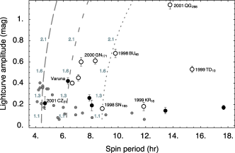
Figure 14.— Lightcurve amplitudes versus spin periods of KBOs. The black filled and open circles represent objects larger and smaller than 400 km, respectively. The smaller gray circles show the results of numerical simulations of “rubble-pile” collisions (Leinhardt et al. 2000). The lines represent the locus of rotating ellipsoidal figures of hydrostatic equilibrium with densities $\rho=500\,{\rm kg}\,{\rm m}^{-3}$ (dotted line), $\rho=1000\,{\rm kg}\,{\rm m}^{-3}$ (shorter dashes) and $\rho=2000\,{\rm kg}\,{\rm m}^{-3}$ (longer dashes). Shown in grey next to the lines are the axis ratios, $a/b$, of the ellipsoidal solutions. Both the Leinhardt et al. (2000) results and the figures of equilibrium assume equator-on observing geometry and therefore represent upper limits.

In this section we wish to investigate if the rotational properties of KBOs show any evidence that they have a rubble pile structure; a possible dependence on object size is also investigated. As in the case of asteroids, collisional evolution may have played an important role in modifying the inner structure of KBOs. Large asteroids ($D\gtrsim 200\,$km) have in principle survived collisional destruction for the age of the solar system, but may nonetheless have been converted to rubble piles by repeated impacts. As a result of multiple collisions, the “loose” pieces of the larger asteroids may have reassembled into shapes close to triaxial equilibrium ellipsoids (Farinella et al. 1981). Instead, the shapes of smaller asteroids ($D\leq 100\,$km) are consistent with collisional fragments (Catullo et al. 1984), indicating that they are most likely by-products of disruptive collisions.

Figure 14 plots the lightcurve amplitudes versus spin periods for the 15 KBOs whose lightcurve amplitudes and spin period are known. Open and filled symbols indicate the KBOs with diameter smaller and larger than $D=400\,$km, respectively. Clearly, the smaller and larger KBOs occupy different regions of the diagram. For the larger KBOs (black filled circles) the (small) lightcurve amplitudes are almost independent of the objects’ spin periods. In contrast, smaller KBOs span a much broader range of lightcurve amplitudes. Two objects have very low amplitudes: $(35671)\,1998\,\rm{SN}_{165}$ and 1999 KR₁₆, which have diameters $D\sim 400\,$km and fall precisely on the boundary of the two size ranges. The remaining objects hint at a trend of increasing $\Delta m$ with lower spin rates. The one exception is 1999 TD₁₀, a Scattered Disk Object ($e=0.872,a=95.703\,$AU) that spends most of its orbit in rather empty regions of space and most likely has a different collisional history.

For comparison, Fig. 14 also shows results of N-body simulations of collisions between “ideal” rubble piles (gray filled circles; Leinhardt et al. 2000), and the lightcurve amplitude-spin period relation predicted by ellipsoidal figures of hydrostatic equilibrium (dashed and dotted lines; Chandrasekhar 1969, Holsapple 2001). The latter is calculated from the equilibrium shapes that rotating uniform fluid bodies assume by balancing gravitational and centrifugal acceleration. The spin rate-shape relation in the case of uniform fluids depends solely on the density of the body. Although fluid bodies behave in many respects differently from rubble piles, they may, as an extreme case, provide insight on the equilibrium shapes of gravitationally bound agglomerates. The lightcurve amplitudes of both theoretical expectations are plotted assuming an equator-on observing geometry. They should therefore be taken as upper limits when compared to the observed KBO amplitudes, the lower limit being zero amplitude.

The simulations of Leinhardt et al. (2000, hereafter LRQ) consist of collisions between agglomerates of small spheres meant to simulate collisions between rubble piles. Each agglomerate consists of $\sim 1000$ spheres, held together by their mutual gravity, and has no initial spin. The spheres are indestructible, have no sliding friction, and have coefficients of restitution of $\sim 0.8$. The bulk density of the agglomerates is 2000 kg m^-3. The impact velocities range from $\sim$ zero at infinity to a few times the critical velocity for which the impact energy would exceed the mutual gravitational binding energy of the two rubble piles. The impact geometries range from head-on collisions to grazing impacts. The mass, final spin period, and shape of the largest remnant of each collision are registered (see Table 1 of LRQ). From their results, we selected the outcomes for which the mass of the largest remnant is equal to or larger than the mass of one of the colliding rubble piles, i.e., we selected only accreting outcomes. The spin periods and lightcurve amplitudes that would be generated by such remnants (assuming they are observed equator-on) are plotted in Fig. 14 as gray circles. Note that, although the simulated rubble piles have radii of 1 km, since the effects of the collision scale with the ratio of impact energy to gravitational binding energy of the colliding bodies (Benz & Asphaug 1999), the model results should apply to other sizes. Clearly, the LRQ model makes several specific assumptions, and represents one possible idealization of what is usually referred to as “rubble pile”. Nevertheless, the results are illustrative of how collisions may affect this type of structure, and are useful for comparison with the KBO data.

The lightcurve amplitudes resulting from the LRQ experiment are relatively small ($\Delta m<0.25\,$mag) for spin periods larger than $P\sim 5.5\,$hr (see Fig. 14). Objects spinning faster than $P=5.5\,$hr have more elongated shapes, resulting in larger lightcurve amplitudes, up to 0.65 magnitudes. The latter are the result of collisions with higher angular momentum transfer than the former (see Table 1 of LRQ). The maximum spin rate attained by the rubble piles, as a result of the collision, is $\sim 4.5\,$hr. This is consistent with the maximum spin expected for bodies in hydrostatic equilibrium with the same density as the rubble piles ($\rho=2000\,$kg m^-3; see long-dashed line in Fig. 14). The results of LRQ show that collisions between ideal rubble piles can produce elongated remnants (when the projectile brings significant angular momentum into the target), and that the spin rates of the collisional remnants do not extend much beyond the maximum spin permitted to fluid uniform bodies with the same bulk density.

The distribution of KBOs in Fig. 14 is less clear. Indirect estimates of KBO bulk densities indicate values $\rho\sim 1000\,$kg m^-3 (Luu & Jewitt 2002). If KBOs are strengthless rubble piles with such low densities we would not expect to find objects with spin periods lower than $P\sim 6\,$hr (dashed line in Fig. 14). However, one object ($2001\,\rm{CZ}_{31}$) is found to have a spin period below 5 hr. If this object has a rubble pile structure, its density must be at least $\sim 2000\,$kg m^-3. The remaining 14 objects have spin periods below the expected upper limit, given their estimated density. Of the 14, 4 objects lie close to the line corresponding to equilibrium ellipsoids of density $\rho=1000\,$kg m^-3. One of these objects, (20000) Varuna, has been studied in detail by Sheppard & Jewitt (2002). The authors conclude that (20000) Varuna is best interpreted as a rotationally deformed rubble pile with $\rho\leq 1000\,$kg m^-3. One object, 2001 QG₂₉₈, has an exceptionally large lightcurve amplitude ($\Delta m=1.14\,$mag), indicative of a very elongated shape (axes ratio $a/b>2.85$), but given its modest spin rate ($P=13.8\,$hr) and approximate size ($D\sim 240\,$km) it is unlikely that it would be able to keep such an elongated shape against the crush of gravity. Analysis of the lightcurve of this object (Sheppard & Jewitt 2004) suggests it is a close/contact binary KBO. The same applies to two other KBOs, 2000 GN₁₇₁ and (33128) 1998 BU₄₈, also very likely to be contact binaries.

To summarize, it is not clear that KBOs have a rubble pile structure, based on their available rotational properties. A comparison with computer simulations of rubble pile collisions shows that larger KBOs ($D>400\,$km) occupy the same region of the period-amplitude diagram as the LRQ results. This is not the case for most of the smaller KBOs ($D\leq 400\,$km), which tend to have larger lightcurve amplitudes for similar spin periods. If most KBOs are rubble piles then their spin rates set a lower limit to their bulk density: one object ($2001\,\rm{CZ}_{31}$) spins fast enough that its density must be at least $\rho\sim 2000\,$kg m^-3, while 4 other KBOs (including (20000) Varuna) must have densities larger than $\rho\sim 1000\,$kg m^-3. A better assessment of the inner structure of KBOs will require more observations, and detailed modelling of the collisional evolution of rubble-piles.

6. Conclusions

We have collected and analyzed R-band photometric data for 10 Kuiper Belt objects, 5 of which have not been studied before. No significant brightness variations were detected from KBOs $(80806)\,2000\,\rm{CM}_{105}$, $(66652)\,1999\,\rm{RZ}_{253}$, $1996\,\rm{TS}_{66}$. Previously observed KBOs $(19521)\,\rm{Chaos}$, $(47171)\,1999\,\rm{TC}_{36}$, and $(38628)\,\rm{Huya}$ were confirmed to have very low amplitude lightcurves ($\Delta m\leq 0.1\,$mag). $(35671)\,1998\,\rm{SN}_{165}$, $(79983)\,1999\,\rm{DF}_{9}$, and $2001\,\rm{CZ}_{31}$ were shown to have periodic brightness variations. Our lightcurve amplitude statistics are thus: 3 out of 10 (30%) observed KBOs have $\Delta m\geq 0.15\,$mag, and 1 out of 10 (10%) has $\Delta m\geq 0.40\,$mag. This is consistent with previously published results.

The rotational properties that we obtained were combined with existing data in the literature and the total data set was used to investigate the distribution of spin period and shapes of KBOs. Our conclusions can be summarized as follows:

1. KBOs with diameters $D>200\,$km have a mean spin period of $9.23\,$hr, and thus rotate slower on average than main belt asteroids of similar size ($\langle P\rangle_{\rm MBAs}=6.48\,$hr). The probability that the two distributions are drawn from the same parent distribution is 0.7%, as judged by the KS test.

2. 26 of 37 KBOs (70%, $D>200\,$km) have lightcurve amplitudes below $0.15\,$mag. In the asteroid belt only 10 of the 27 (37%) asteroids in the same size range have such low amplitude lightcurves. This difference is significant at the 99.2% level according to the Fisher exact test.

3. KBOs with diameters $D>400\,$km have lightcurves with significantly (98.5% confidence) smaller amplitudes ($\langle\Delta m\rangle=0.13\,$mag, $D>400\,$km) than KBOs with diameters $D\leq 400\,$km ($\langle\Delta m\rangle=0.25\,$mag, $D\leq 400\,$km).

4. These two size ranges seem to have different shape distributions, but the few existing data do not render the difference statistically significant. Even though the shape distributions in the two size ranges are not inconsistent, the best-fit power-law solutions predict a larger fraction of round objects in the $D>400\,$km size range ($f(a/b<1.2)\sim 70^{+12}_{-19}\%$) than in the group of smaller objects ($f(a/b<1.2)\sim 42^{+20}_{-15}\%$).

5. The current KBO lightcurve data are too sparse to allow a conclusive assessment of the inner structure of KBOs.

6. KBO $2001\,\rm{CZ}_{31}$ has a spin period of $P=4.71\,$hr. If this object has a rubble pile structure then its density must be $\rho\gtrsim 2000\,$kg m^-3. If the object has a lower density then it must have internal strength.

The analysis presented in this paper rests on the assumption that the available sample of KBO rotational properties is homogeneous. However, in all likelihood the database is biased. The most likely bias in the sample comes from unpublished flat lightcurves. If a significant fraction of flat lightcurves remains unreported then points 1 and 2 above could be strengthened, depending on the cause of the lack of brightness variation (slow spin or round shape). On the other hand, points 3 and 4 could be weakened if most unreported cases correspond to smaller KBOs. Better interpretation of the rotational properties of KBOs will greatly benefit from a larger and more homogeneous dataset.

References

- Benz & Asphaug (1999) Benz, W. & Asphaug, E. 1999, Icarus, 142, 5
- Bernstein et al. (2004) Bernstein, G. M., Trilling, D. E., Allen, R. L., Brown, M. E., Holman, M., & Malhotra, R. 2004, AJ, 128, 1364
- Bertin & Arnouts (1996) Bertin, E. & Arnouts, S. 1996, A&AS, 117, 393
- Brown et al. (1999) Brown, R. H., Cruikshank, D. P., & Pendleton, Y. 1999, ApJ, 519, L101
- Brown et al. (2005) Brown, M. E., Trujillo, C. A., & Rabinowitz, D. L. 2005, ApJ, in press
- Catullo et al. (1984) Catullo, V., Zappala, V., Farinella, P., & Paolicchi, P. 1984, A&A, 138, 464
- Chandrasekhar (1969) Chandrasekhar, S. 1969, Ellipsoidal figures of equilibrium (The Silliman Foundation Lectures, New Haven: Yale University Press, 1969)
- Collander-Brown et al. (1999) Collander-Brown, S. J., Fitzsimmons, A., Fletcher, E., Irwin, M. J., & Williams, I. P. 1999, MNRAS, 308, 588
- Davies et al. (1997) Davies, J. K., McBride, N., & Green, S. F. 1997, Icarus, 125, 61
- Doressoundiram et al. (2002) Doressoundiram, A., Peixinho, N., de Bergh, C., Fornasier, S., Thébault, P., Barucci, M. A., & Veillet, C. 2002, AJ, 124, 2279
- Efron (1979) Efron, B. 1979, Annals of Statistics, 7, 1
- Farinella et al. (1981) Farinella, P., Paolicchi, P., Tedesco, E. F., & Zappala, V. 1981, Icarus, 46, 114
- Farinella et al. (1982) Farinella, P., Paolicchi, P., & Zappala, V. 1982, Icarus, 52, 409
- Goldreich et al. (2002) Goldreich, P., Lithwick, Y., & Sari, R. 2002, Nature, 420, 643
- Grundy et al. (2005) Grundy, W. M., Noll, K. S., & Stephens, D. C. 2005, Icarus, 176, 184
- Hainaut et al. (2000) Hainaut, O. R., Delahodde, C. E., Boehnhardt, H., Dotto, E., Barucci, M. A., Meech, K. J., Bauer, J. M., West, R. M., & Doressoundiram, A. 2000, A&A, 356, 1076
- Holsapple (2001) Holsapple, K. A. 2001, Icarus, 154, 432
- Jewitt et al. (2001) Jewitt, D., Aussel, H., & Evans, A. 2001, Nature, 411, 446
- Jewitt & Luu (1993) Jewitt, D. & Luu, J. 1993, Nature, 362, 730
- Jewitt & Luu (2000) Jewitt, D. C. & Luu, J. X. 2000, Protostars and Planets IV, 1201
- Jewitt & Luu (2001) —. 2001, AJ, 122, 2099
- Jewitt & Sheppard (2002) Jewitt, D. C. & Sheppard, S. S. 2002, AJ, 123, 2110
- Lacerda & Luu (2003) Lacerda, P. & Luu, J. 2003, Icarus, 161, 174
- Leinhardt et al. (2000) Leinhardt, Z. M., Richardson, D. C., & Quinn, T. 2000, Icarus, 146, 133
- Luu & Jewitt (1996) Luu, J. & Jewitt, D. 1996, AJ, 112, 2310
- Luu & Lacerda (2003) Luu, J. & Lacerda, P. 2003, Earth Moon and Planets, 92, 221
- Luu & Jewitt (1998) Luu, J. X. & Jewitt, D. C. 1998, ApJ, 494, L117
- Luu & Jewitt (2002) —. 2002, ARA&A, 40, 63
- Noll et al. (2002) Noll, K. S., Stephens, D. C., Grundy, W. M., Millis, R. L., Spencer, J., Buie, M. W., Tegler, S. C., Romanishin, W., & Cruikshank, D. P. 2002, AJ, 124, 3424
- Ortiz et al. (2003) Ortiz, J. L., Gutiérrez, P. J., Sota, A., Casanova, V., & Teixeira, V. R. 2003, A&A, 409, L13
- Ortiz et al. (2001) Ortiz, J. L., Lopez-Moreno, J. J., Gutierrez, P. J., & Baumont, S. 2001, BAAS, 33, 1047
- Peixinho et al. (2002) Peixinho, N., Doressoundiram, A., & Romon-Martin, J. 2002, New Astronomy, 7, 359
- Romanishin & Tegler (1999) Romanishin, W. & Tegler, S. C. 1999, Nature, 398, 129
- Romanishin et al. (2001) Romanishin, W., Tegler, S. C., Rettig, T. W., Consolmagno, G., & Botthof, B. 2001, BAAS, 33, 1031
- Rousselot et al. (2003) Rousselot, P., Petit, J.-M., Poulet, F., Lacerda, P., & Ortiz, J. 2003, A&A, 407, 1139
- Sheppard & Jewitt (2004) Sheppard, S. S. & Jewitt, D. 2004, AJ, 127, 3023
- Sheppard & Jewitt (2002) Sheppard, S. S. & Jewitt, D. C. 2002, AJ, 124, 1757
- Sheppard & Jewitt (2003) —. 2003, Earth Moon and Planets, 92, 207
- Stellingwerf (1978) Stellingwerf, R. F. 1978, ApJ, 224, 953
- Tegler & Romanishin (2000) Tegler, S. C. & Romanishin, W. 2000, Nature, 407, 979
- Torppa et al. (2003) Torppa, J., Kaasalainen, M., Michalowski, T., Kwiatkowski, T., Kryszczyńska, A., Denchev, P. & Kowalski, R. 2003, Icarus, 164, 346
- Trujillo & Brown (2002) Trujillo, C. A. & Brown, M. E. 2002, ApJ, 566, L125
- Trujillo et al. (2001a) Trujillo, C. A., Jewitt, D. C., & Luu, J. X. 2001a, AJ, 122, 457
- Trujillo et al. (2001b) Trujillo, C. A., Luu, J. X., Bosh, A. S., & Elliot, J. L. 2001b, AJ, 122, 2740
- van Dokkum (2001) van Dokkum, P. G. 2001, PASP, 113, 1420
- Weidenschilling (2002) Weidenschilling, S. J. 2002, Icarus, 160, 212