Automated analysis of eclipsing binary lightcurves with EBAS. II. Statistical analysis of OGLE LMC eclipsing binaries

Abstract

In the first paper of this series we presented EBAS, a new fully automated algorithm to analyse the lightcurves of eclipsing binaries, based on the EBOP code. Here we apply the new algorithm to the whole sample of 2580 binaries found in the OGLE LMC photometric survey and derive the orbital elements for 1931 systems. To obtain the statistical properties of the short-period binaries of the LMC we construct a well defined subsample of 938 eclipsing binaries with main-sequence B-type primaries. Correcting for observational selection effects, we derive the distributions of the fractional radii of the two components and their sum, the brightness ratios and the periods of the short-period binaries. Somewhat surprisingly, the results are consistent with a flat distribution in log P between 2 and 10 days. We also estimate the total number of binaries in the LMC with the same characteristics, and not only the eclipsing binaries, to be about 5000. This figure leads us to suggest that $(0.7\pm 0.4)$% of the main-sequence B-type stars in the LMC are found in binaries with periods shorter than 10 days. This frequency is substantially smaller than the fraction of binaries found by small Galactic radial-velocity surveys of B stars. On the other hand, the binary frequency found by HST photometric searches within the late main-sequence stars of 47 Tuc is only slightly higher and still consistent with the frequency we deduced for the B stars in the LMC.

1 Introduction

A number of large photometric surveys have recently produced unprecedentedly large sets of high S/N stellar lightcurves (e.g., Alcock et al., 1997). One of these projects is the OGLE study of the SMC (Udalski et al., 1998) and the LMC (Udalski et al., 2000), which has already yielded (Wyrzykowski et al., 2003) a few thousand lightcurves of eclipsing binaries. These two sets of lightcurves enable a statistical analysis of a large sample of short-period extragalactic binaries, for which the absolute magnitudes of all systems are known to a few percent. No such sample is known in our Galaxy.

One such statistical study was the analysis of North & Zahn (2003), who derived the orbital elements and stellar parameters of 153 eclipsing binaries discovered by OGLE in the SMC. North & Zahn examined the eccentricities of the eclipsing binaries as a function of the ratio between the stellar radii and the binary separation, and compared their result with a similar dependence derived from the elements of the binaries discovered by Alcock et al. (1997) in the LMC. They then considered the implication of their findings for the theory of tidal circularization of early-type primaries in close binaries (e.g., Zahn, 1975, 1977; Zahn & Bouchet, 1989).

In a follow-up paper North & Zahn (2004) analyzed another set of 510 lightcurves selected from the 2580 eclipsing binaries discovered in the LMC by the OGLE team (Wyrzykowski et al., 2003). Again, they derived the ratio between the stellar radii and the binary separation for these systems, and examined the dependence of the binary eccentricity on this ratio.

The previous analyses used only a small fraction of the sample of eclipsing binaries found in the OGLE data. The goal of the present study is to analyze the whole sample of 2580 lightcurves discovered by OGLE in the LMC, and to derive some statistical properties of the short-period binaries, after correcting for observational selection effects. Such a correction is essential for the derivation of the period distribution, for example, because the probability of detecting an eclipsing binary is a strong function of the orbital period. In order to apply an appropriate correction one needs a complete homogeneous data set of lightcurves, all discovered by the same photometric survey of a well defined sample of stars. These requirements were exactly met by the OGLE data set for the LMC, enabling such analysis for a large sample of eclipsing binaries for the first time.

A completely automated algorithm is needed to analyse the large set of eclipsing binaries at hand. Two such codes were developed recently. Wyithe & Wilson (2001) have constructed an automatic scheme based on the Wilson-Divenney (=WD) code to analyze the OGLE lightcurves detected in the SMC in order to find eclipsing binaries suitable for distance measurements. At the last stages of writing this paper another study with an automated lightcurve fitter — DEBiL, was published (Devor, 2005). DEBiL was constructed to be quick and simple, and therefore has its own lightcurve generator, which does not account for stellar deformation and reflection effects. This makes it especially suitable for detached binaries. We will use in this work our EBAS, which was presented in Paper I (Tamuz, Mazeh & North 2005) and is based on the EBOP code. The complexity of EBAS is in between DEBiL and the automated WD code of Wyithe & Wilson.

To facilitate the search for global minima in the convolved parameter space, EBAS performs two parameter transformations. Instead of the radii of the two stellar components of the binary system, measured in terms of the binary separation, EBAS uses the total radius, which is the sum of the two relative radii, and their ratio. Instead of the inclination we use the impact parameter — the projected distance between the centres of the two stars in the middle of the primary eclipse, measured in terms of the total radius.

The set of parameters of the EBAS version used here includes the bolometric reflection of the two stars, $A_{p}$ and $A_{s}$. When $A_{p}=1$ the primary star reflects all the light cast on it by the secondary. Together with the tidal distortion of the two components, which is mainly determined by the mass ratio of the two stars, the reflection coefficients $A_{p}$ and $A_{s}$ determine the light variability of the system outside the eclipses. Paper I discussed the reliability of the values of these two parameters as found by EBAS.

To simplify the analysis, the present version of EBAS assumes there is no contribution of light from a third star and that the mass ratio is unity. Paper I discusses the implication of these choices on the parameters’ values, showing that the values of the total radius and the surface brightness ratio are only slightly modified by these two assumptions. The only parameter which is systematically modified by the third-light assumption is the impact parameter, which is directly associated with the orbital inclination of the binary. Note, however, that we are not interested in one specific system but aim, instead, at deriving the gross characteristics of the short-period binaries. As the analysis of this paper does not use the inclinations of the eclipsing binaries for the derivation of the statistical features of the short-period binaries, we regard the resulting distributions as probably correct.

Paper I introduces a new ’alarm’ statistic, $\mathcal{A}$, to replace human inspection of the residuals. EBAS uses the new statistic, which is sensitive to the correlation between neighbouring residuals to decide automatically whether a solution is satisfactory. In this work we consider only the 1931 systems that yielded solutions with low enough alarm value.

To check the reliability of our results we compare our geometrical elements with those derived by Michalska & Pigulski (2005, hereafter MiP05) with the WD code for 85 binaries, based on EROS, MACHO and OGLE data. The comparison is reassuring, as it shows that the geometrical parameters of EBAS are close to the ones derived by the more sophisticated WD approach.

To derive the orbital distributions of the short-period binaries we had to trim the sample, to get a homogeneous sample which we could correct for selection effects. We were left with 938 main-sequence binaries with periods shorter than 10 days and system magnitudes between 17 and 19 in the $I$ band, most of which are binaries with B-type primaries. This makes the range of the derived period distribution quite narrow. Nevertheless, the data yielded somewhat surprising distributions, which might have implications on binary population studies.

Section 2 presents the resulting orbital elements of the OGLE LMC eclipsing binaries and compares the derived elements with those of MiP05. Section 3 details the procedure to focus on a well defined homogeneous subsample and Section 4 derives the statistical features of the short-period binaries, after correcting for the observational selection effects. Section 5 discusses the new findings, and Section 6 summarizes the paper.

2 Analysis of the OGLE LMC Eclipsing Binaries

The LMC OGLE-II photometric campaign (Udalski et al., 2000) was carried out from 1997 to 2000, during which between 260 and 512 measurements in the $I$ band were taken for 21 fields (Zebrun et al., 2001). Wyrzykowski et al. (2003) searched the photometric data base and identified 2580 binaries. We analysed those systems with EBAS and found 1931 acceptable solutions. Three types of binaries were excluded:

• Four binaries were found to appear twice in the list of binaries, with the same period (except for a factor of 2) and with very close positions. Apparently, they originated from the overlap between the different fields of OGLE, and evaded the scrutiny of Wyrzykowski et al. (2003).

• EBAS found 376 solutions with alarm too high — $\mathcal{A}>0.5$. Visual inspection showed that most of these systems are contact binaries that EBOP can not model properly. Some might be ellipsoidal variables (see Wyrzykowski et al., 2003) or other types of periodic variables, other than eclipsing binaries.

• EBAS found 269 solutions that yielded sum of radii $r_{t}=r_{p}+r_{s}$ too large. Following the Roche lobe radius calculation in Eggleton (1983):

  $$R_{RL}/a=\frac{0.49\,q^{2/3}}{0.6\,q^{2/3}+\ln(1+q^{1/3})}\;\;,$$ (1)

  which reduces for $q=1$ to $R_{RL}/a=0.379$, we did not accept solutions with

  $$r_{t}>0.65\,(1-e\cos\omega)\ ,$$ (2)

  assuming the EBOP model can not properly account for the deformation of the two stars if one or two stars are too close to their Roche-lobe limit, at least at the periastron passage.

We were thus left with 1931 acceptable solutions.

2.1 Solution examples

In Fig 1 we plot 10 representative lightcurves derived by the EBAS. Their elements are given in Table 1 and Table 2. Table 1 gives some global information on each lightcurve and the goodness-of-fit of its model. It lists the number of measurements, the averaged observed $I$-magnitude and the rms of the scatter of the OGLE lightcurve. It also lists the $\chi^{2}$, the alarm $\mathcal{A}$ of the fit and the detectability measure $\mathcal{D}$ (see below), and whether this binary was included in the trimmed sample (+), as detailed in the next section. Table 2 lists the derived elements of EBAS and their estimated uncertainties. This includes the $I$-magnitude of the system at quadrature (the $SFACT$ parameter of EBOP, see Table 2 of Paper I), the period, $P$, in days, the sum of radii, $r_{t}$, the ratio of radii, $k$, the surface brightness ratio, $J_{s}$, the impact parameter, $x$, and the eccentricity $e$, multiplied by $\cos\omega$ and $\sin\omega$, where $\omega$ is the longitude of periastron. Note that the mag parameter in Table 2 is the brightness of the system out of eclipse, and therefore is different from the observed averaged mag given in Table 1. Since its formal error is very small, we give it to 4 or 5 decimal figures because this might be useful for comparison purposes, even though we are well aware that systematic errors — whether in the original photometric data or in their fit — are far larger than that level of accuracy. Let us recall that some parameters were held fixed in the fit, as explained in Paper I: the linear limb-darkening coefficients, with a value typical of main-sequence B stars ($u_{p}=u_{s}=0.18$), the gravity darkening coefficients ($y_{p}=y_{s}=0.36$), the mass ratio ($q=1$), the tidal lead/lag angle ($t=0$) and the third light ($L_{3}=0$). $A_{p}$ and $A_{s}$ are the bolometric reflection coefficients, the value of which is between $0$ and $1$; they determine (together with the tidal distorsion of the components) the out-of-eclipse variability. They are adjusted in order to fit the variation outside eclipses, but since reflection effects are only crudely modeled by EBOP, one has to keep in mind that their value may have very limited physical significance.

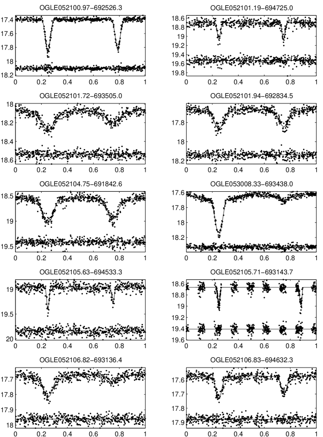
Figure 1: Ten derived lightcurves

Table 1: The ten binaries: observations and goodness-of-fit

OGLE Name	$N$	$mag$	$rms$	$\chi^{2}$	$\mathcal{A}$	$\log\mathcal{D}$	Sample
052100.97-692526.3	482	17.44	0.12	397	-0.3	15015	+
052101.19-694725.0	478	18.73	0.09	453	-0.2	688	+
052101.72-693505.0	479	18.12	0.07	381	0.1	1606
052101.94-692834.5	472	17.70	0.06	335	-0.1	1969	+
052104.75-691842.6	479	18.64	0.16	425	-0.0	3658	+
053008.33-693438.0	507	17.69	0.11	410	0.4	12503	+
052105.63-694533.3	477	18.98	0.10	376	0.1	660	+
052105.71-693143.7	482	18.71	0.10	401	-0.2	1540	+
052106.82-693136.4	478	17.69	0.04	299	0.0	1353
052106.83-694632.3	481	17.59	0.04	353	0.2	1704	+

Table 2: The ten binaries: orbital elements

OGLE Name	$mag$	$P$	$r_{t}$	$k$	$J_{s}$	$x$	$e\cos\omega$	$e\sin\omega$	$A_{p}$	$A_{s}$
052100.97	17.39743	3.1227063	0.2968	0.80	0.934	0.233	0.05902	0.0041	0.73	1.00000
-692526.3	$\pm$0.00095	$\pm$0.0000061	$\pm$0.0038	$\pm$0.26	$\pm$0.015	$\pm$0.018	$\pm$0.00066	$\pm$0.0093	$\pm$0.18	$\pm$0.00026
052101.19	18.7058	9.156860	0.1788	1.16	0.97	0.339	-0.0038	0.005	0.9999	0.99993
-694725.0	$\pm$0.0025	$\pm$0.000051	$\pm$0.0086	$\pm$0.37	$\pm$0.13	$\pm$0.062	$\pm$0.0014	$\pm$0.057	$\pm$0.0013	$\pm$0.00090
052101.72	18.0867	1.4570012	0.674	1.31	0.65	0.696	0.0016	0.004	0.75	0.916
-693505.0	$\pm$0.0015	$\pm$0.0000070	$\pm$0.024	$\pm$0.26	$\pm$0.11	$\pm$0.016	$\pm$0.0042	$\pm$0.012	$\pm$0.20	$\pm$0.099
052101.94	17.6753	1.3626777	0.560	1.02	0.954	0.607	0.0003	0.011	1.000	0.998
-692834.5	$\pm$0.0015	$\pm$0.0000025	$\pm$0.015	$\pm$0.10	$\pm$0.069	$\pm$0.019	$\pm$0.0029	$\pm$0.017	$\pm$0.013	$\pm$0.054
052104.75	18.5378	1.7568736	0.534	1.65	0.895	-0.035	0.0002	-0.018	0.55	0.11
-691842.6	$\pm$0.0023	$\pm$0.0000041	$\pm$0.016	$\pm$0.48	$\pm$0.038	$\pm$0.094	$\pm$0.0032	$\pm$0.028	$\pm$0.31	$\pm$0.28
053008.33	17.6360	4.136428	0.4594	4.86	0.065	0.736	0.0006	-0.061	0.01	0.945
-693438.0	$\pm$0.0010	$\pm$0.000015	$\pm$0.0092	$\pm$0.51	$\pm$0.018	$\pm$0.026	$\pm$0.0052	$\pm$0.028	$\pm$0.16	$\pm$0.099
052105.63	18.9528	6.7992460	0.1450	0.80	0.757	0.275	0.0018	-0.002	1.0000	0.990
-694533.3	$\pm$0.0029	$\pm$0.0000035	$\pm$0.0074	$\pm$0.26	$\pm$0.076	$\pm$0.047	$\pm$0.0021	$\pm$0.066	$\pm$0.0011	$\pm$0.038
052105.71	18.6663	8.000289	0.1147	1.8	0.987	0.22	0.2069	-0.060	1.00	0.095
-693143.7	$\pm$0.0022	$\pm$0.000029	$\pm$0.0053	$\pm$1.8	$\pm$0.089	$\pm$0.13	$\pm$0.0012	$\pm$0.042	$\pm$0.20	$\pm$0.040
052106.82	17.6869	1.6991553	0.591	1.20	0.362	0.780	0.0015	0.031	0.988	0.820
-693136.4	$\pm$0.0011	$\pm$0.0000086	$\pm$0.017	$\pm$0.12	$\pm$0.094	$\pm$0.018	$\pm$0.0079	$\pm$0.022	$\pm$0.022	$\pm$0.087
052106.83	17.5775	4.796268	0.379	1.40	0.64	0.686	0.0029	-0.038	0.99	0.79
-694632.3	$\pm$0.0011	$\pm$0.000024	$\pm$0.010	$\pm$0.24	$\pm$0.22	$\pm$0.035	$\pm$0.0024	$\pm$0.055	$\pm$0.15	$\pm$0.20

Of the ten stars, the lightcurve of OGLE052101.72-693505 yielded $r_{t}$ too high, and the primary of OGLE052106.82-693136.4 is probably not a main-sequence star (see below). Therefore both stars were not included in the final statistical analysis. Because the system 053008.33-693438.0 has a very shallow secondary minimum, its ratio of radii is poorly constrained, and it probably has undergone mass exchange. Because of the very small surface brightness ratio, the reflection coefficient is meaningful for the secondary but not for the primary, which remains unaffected by the presence of its much cooler companion. Thus the very small $A_{p}$ value has no real meaning.

The elements of all 1931 binaries are given in Table 3 and Table 4 with exactly the same format as in Table 1 and Table 2. Tables 3 & 4 appear only in electronic version of the journal in postscript format, while their machine-readable ASCII version is available in our web site.

2.2 Comparison with the analysis of Michalska & Pigulski (2005)

In Paper I we compared the elements of four systems derived by EBAS with those obtained by González et al. (2005). Here we wish to compare our results with the more extensive work of MiP05 published very recently. Using data from EROS, MACHO and OGLE, MiP05 fitted 98 LMC binaries with the WD code. Of those, 85 were included in the OGLE catalogue and 81 were solved by EBAS with low $\mathcal{A}$.

Because of the differences between WD and EBOP, we wish to compare only the geometric parameters of the solutions (see Paper I). Plotted in Fig 2 are our values for the 81 binaries versus MiP05’s, for the sum of radii, inclination and eccentricity. The total radius and the eccentricity panels show quite small spread around the straight lines, which represent the locus of equal values of the two solutions. Only the inclination shows a large scatter and a slight bias. However, as noted above, our statistical analysis does not use the inclinations of the eclipsing binaries for the derivation of the characteristics of the short-period binaries. Therefore, the comparison with MiP05’s solutions supports our assessment that while individual EBAS solutions might be inferior to WD solutions, the statistical interpretation of the entire sample remains valid.

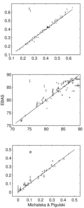
Figure 2: Comparison with the work of MiP05: Elements for 81 systems. Panels are for sum of radii, inclination and eccentricity

3 Trimming the sample

The very large sample of 1931 short-period binaries enables us to derive some statistical features of the population of short-period binaries in the LMC. However, the sample suffers from serious observational selection effects, which affected the discovery of the eclipsing binaries. To be able to correct for the selection effects we need a well-defined homogeneous sample. We therefore trim the sample before deriving some parameter distributions in the next section.

The most important observational selection effect is associated with the weak signal of the eclipse relative to the noise of the measurements. To apply a correction for this selection effect we need a distinct criterion that defines the systems that could have been detected by the OGLE LMC survey. Such a criterion is the detectability parameter $\mathcal{D}$, which we define to be the number of points in the lightcurve, $N$, times the ratio of the variance of the ideal but variable signal, to the variance of the residuals:

$$\mathcal{D}=N\frac{var(m_{i})}{var(r_{i})}\ .$$ (3)

The $m_{i}$’s are the values of the EBAS model at the times of observation, and the $r_{i}$’s are the residuals of the measurements relative to the model. One sees that systems with deep eclipses, which are more easily detected, have larger $\mathcal{D}$, and even more so when many measurements are concentrated within phases of eclipses.

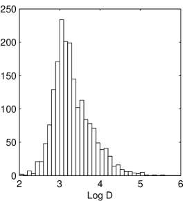
Figure 3: Distribution of the detectability parameter $\log\mathcal{D}$ for the 1931 binaries with acceptable solutions.

Fig 3 shows the distribution of $\log\mathcal{D}$ for all 1931 solved systems. The histogram shows that there are only very few systems with $\log\mathcal{D}$ below $2.6$. We therefore set our detection limit, somewhat arbitrarily, at $\log\mathcal{D}=2.6$, assuming that any binary below this limit could not have been detected. As pointed out by the referee, this limit translates into $\mathcal{D}=400$, which implies a $1\sigma$ variation in a lightcurve having $400$ points — a rather typical number. We consider the few systems below this limit as exceptions. In order to get a homogeneous sample we ignore the binaries below this limit, and consider only the 1875 systems with $\log\mathcal{D}>2.6$.

Fig 4 shows the total magnitude of the binaries left in the sample as a function of their orbital periods. We are witnessing a lack of systems in the lower right corner of the plot. This is due to the fact that the probability of having an eclipse is approximately equal to the sum of fractional radii, $r_{t}$. The two absolute radii determine the total luminosity of their system, while the binary separation determines the orbital period. Therefore, for a given period, the probability of having an eclipse is smaller for faint systems, with smaller stellar radii, than for brighter systems, with larger stars. In addition, the detectability $\mathcal{D}$ is smaller for fainter systems which have larger $var(r_{i})$, making fainter systems less frequent in the sample.

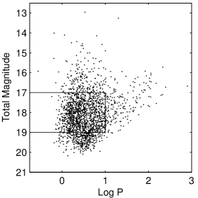
Figure 4: Total $I$-magnitude vs. period for 1875 binaries with accepted solutions and high enough detectability. The straight lines present the limits of the trimmed sample. Periods are in days

In order to obtain a sample that does not suffer from severe incompleteness, we chose, somewhat arbitrarily, to consider only systems in the range of total magnitude between 17 and 19 and with periods shorter than 10 days. The selected range, which included 1131 systems, is denoted in the figure.

For a distance modulus of $\mu_{0}=18.50\pm 0.02$ (Alves, 2004), the trimmed sample range is between absolute $I$-magnitude of $-$1.5 and 0.5, if interstellar absorption is neglected. For a metallicity $Z=0.008$ (typical of the LMC), this range corresponds, for single stars at ZAMS, to spectral type between B1 and B6 and mass range between 8.7 and 3.6 $M_{\odot}$ (Schaerer et al., 1993). Obviously, if the two stars have close to equal luminosities, the primary could be as faint as 1.2 in $I$, which corresponds to a B8 spectral type.

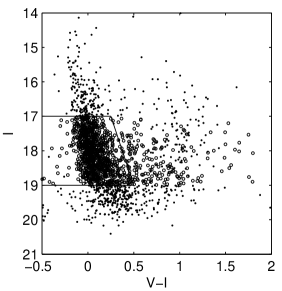
Figure 5: The $I$-magnitude as a function of the averaged $V-I$ colour. Binaries excluded from the trimmed sample by the previous constraints are represented by dots. All 1131 binaries still in the trimmed sample are presented by small circles.

Finally, we calculated for all binaries the averaged $V-I$ colour index. This was calculated by averaging all $V$ measurements that were observed in the phase between 0.15 and 0.35 and 0.65 and 0.85, that is out of eclipse. The $I$-magnitude of each system was taken from the orbital solution. Fig 5 presents for the 1931 binaries with reliable elements the $I$-magnitude as a function of the averaged $V-I$ colour. Obviously, most binaries are on the main sequence, but some binaries are not. We excluded the binaries out of the plotted lines and were left with 938 binaries. This is the trimmed sample that the next section uses for the statistical analysis of the short-period binaries in the LMC.

4 Statistical analysis of the trimmed sample

4.1 The radii and the surface brightness ratio distributions

In order to study the statistical features of the short-period binaries in the LMC with mainly B-type main-sequence primaries, we plotted in Fig 6 the distribution of four orbital elements derived for the trimmed eclipsing binary sample. This includes the surface brightness ratio of the two stars, the fractional primary and secondary radii, and the sum of the two radii.

The distributions are represented by histograms, which were derived by the Gaussian kernel method (e.g., Silverman, 1986). Each binary is represented by a normal distribution centred on the derived value of its parameter, with a width equal to the estimated uncertainty of the parameter. Therefore, each of the histograms represents a sum of normal distributions, differing in mean and variance. The error bars in the histogram bins are just the square root of the value of each bin, assuming Poisson statistics.

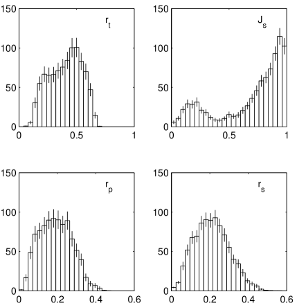
Figure 6: Histogram of the derived elements.

Obviously, the observed distributions are highly convoluted by selection effects. For example, binary systems with longer periods must have an inclination closer to $90^{\circ}$ to be detected as an eclipsing binary. To correct for this effect, we calculated for each system the minimum inclination for which the eclipse could still be detected. This was done by calculating for each system the minimum inclination $i_{min}$ for which the produced eclipse would still be above the detection threshold, given the physical parameters of the two stellar components and the binary elements. We assumed a lightcurve is detectable whenever $\log\mathcal{D}>2.6$, as above.

Assuming the systems are randomly oriented in space, the probability of an inclination to fall between $i_{min}$ and $90^{\circ}$ is $p=\cos i_{min}$. To account for systems with inclinations outside this range, we considered each system as representing $1/p$ binaries, and drew the different histograms accordingly.

Actually, the probability of detection might also be a function of the phase of the primary eclipse, especially if the data points are not equally distributed over the binary phase and the period is close to an integer number of days (See the discussion of Pont et al. (2005) and in particular their Figure 12). We therefore averaged each $p$ over 100 different phases of the primary eclipse, and only then assigned each system with $1/p$ binaries.

The histograms of the “weighted” binaries are shown in Fig 7. The error bars of each bin were calculated by taking the square root of the sum of squares of the $1/p$ values of that bin.

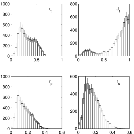
Figure 7: Histogram of the elements, corrected for the observational selection effect

The histograms of the primary and secondary radii show a dramatic rise between 0.05 and 0.1, and a moderate linear decrease between 0.1 and 0.4. The distribution of the surface brightness ratios has a maximum at about unity and decreases monotonically down to about $0.5\pm 0.1$; then it reverses its trend, rising to a secondary, small maximum at about 0.2.

The histogram of the surface brightness ratios reflects the mass-ratio distribution of the whole population of short-period binaries with early-type primaries. This is especially true for main-sequence stars, where for a given primary star the surface brightness ratio of a binary is a monotonic function of its mass ratio. Therefore, the small local secondary maximum at 0.2 is of particular interest, because it might be an indication for a similar local maximum in the mass-ratio distribution.

However, the local maximum of the surface brightness ratio distribution could have been caused by binaries that have gone through mass transfer. Such binaries should have relatively short periods. To follow the nature of the local small maximum we plotted in Fig 8 the corrected histograms only for the binaries with $\log P>0.5$. The secondary peak at the distribution of the surface brightness ratios almost disappears, and the histogram decreases quite monotonically from the peak at unity. We, therefore, suggest that the initial mass-ratio distribution of the short-period binaries with B-type primaries rises monotonically up to a mass ratio of unity.

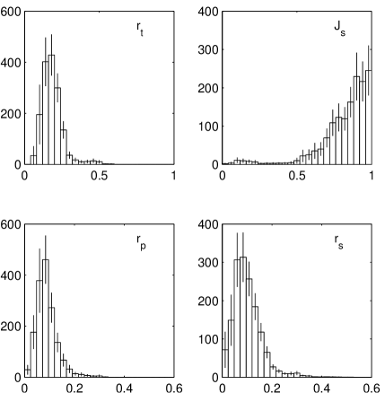
Figure 8: The same histograms as in Fig 7, for binaries with $\log P>0.5$

4.2 The period distribution

To study the period distribution of the binaries in the LMC we plotted in Fig 9 period histograms of the trimmed sample, before and after the correction for the observational effects was applied. We emphasize that if the correction was applied properly, the lower panel represents the period distribution of all binaries in the LMC with $I$-magnitude between 17 and 19, and with sum of radii smaller than about 0.6, and not only the eclipsing binaries.

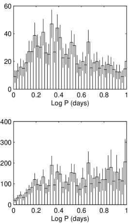
Figure 9: The period distribution of the binaries in the LMC. The top panel shows the period histogram of the trimmed sample, while the lower one shows the corrected histogram

The corrected period histogram shows clearly a distribution that rises up to about $\log P=0.3$, and then flattens off. However, before we conclude that this is the actual distribution of short-period binaries we have to consider another possible selection effect, which is associated with the fact that the fractional length of an eclipse is shorter for long-period binaries than for short-period binaries. This effects turns the number of observations within an eclipse to be smaller for long-period binaries than for short-period binaries. Therefore, for the same two stellar components and eclipse depth, the signal associated with the eclipse is smaller for binaries with long periods than for those with short periods. Consequently, the minimum secondary radius that can be detected might be a function of the binary period. This might reduce the number of binaries discovered with long periods.

However, this selection effect can be substantial only for stars with small relative radii. Eclipsing binaries in our sample, with secondary radii larger than 0.03 and primary ones in the range 0.1–0.2, can be detected easily for periods of 10 days. We therefore suggest that the eclipse length effect should be quite small in our sample. To further check this point we calculated how an assumed flat log distribution between 2 and 10 days would be affected by the eclipse length effect. To do that we took all the 143 binaries in the sample with $0.3<\log P<0.4$ and checked their detectability if we change their period to be 10 days and their inclination to be $90^{\circ}$. Only eight binaries lost their detectability because of the eclipse length effect. This means that the implication of this effect is less than 6%.

We therefore conclude that the period distribution of the short-period binaries is consistent with a flat log distribution between 2 and 10 days.

4.3 The frequency of the short-period binaries

As stated above, the corrections we apply allow us to study the distributions of all short-period binaries, up to 10 days, and not only the eclipsing binaries. We wish to take advantage of this feature of our analysis and estimate, within the limits of the sample, the total number of binaries in the LMC and their fractional frequency.

The sum of weights of the 938 binaries in the trimmed sample is 4585. This means that we estimate there are 4585 short-period binaries in the LMC that fulfil the constraints we have on the trimmed sample. To get the total number of binaries with periods shorter than 10 days we have to add the high-alarm binaries and the ones with large radii; since the added systems are close binaries, their detection probability reaches almost 1 so we do not correct for it in their case. When we add those we end up with 5004 binaries.

We therefore suggest that the number of binaries in the LMC, with period shorter than 10 days, with $I$ between 17 and 19, and for which the $V-I$ colour of the system indicates a main-sequence primary, is about 5000.

Our estimate is valid as far as Wyrzykowski et al. (2003) detected all eclipsing binaries and classified them as such, rather than as other types of variables (e.g. small amplitude cepheids). We do correct for the detection probability, including for the effect of phase of minima, but still assumed that each binary has been correctly identified. One could imagine that 10 to 30% of the potentially detectable binaries were missed for some reason, but hardly much more. We, therefore, arbitrarily assign an error of 30% to the number of binaries in the sample.

We have shown that our sample consists mainly of B-type main-sequence binaries. In order to estimate the fractional frequency of B-type main-sequence stars which reside in binaries that could have been detected by OGLE we have to estimate how many main-sequence single stars were found by OGLE in the same range of magnitudes and colours. To do that, we applied exactly the same procedure we performed above to the whole OGLE dataset of LMC stars in the 21 OGLE fields and found 332,297 main-sequence stars in the $I$-range of 17–19. However, the luminosity of a binary is brighter than the luminosity of its primary by a magnitude that depends on the light ratio of the two stars of the system. Therefore, to consider a population of single stars which is about equal to the population of the primaries of our binary sample we considered instead the range between 17.5 and 19.5 $I$-magnitude, and found 705,535 stars. Taking into account about 1% overlap between the OGLE fields, we adopt 700,000 as a representative number of single stars in the LMC similar to the population of our binary sample. We arbitrarily assign an error of 50% to this figure.

We therefore conclude that $(0.7\pm 0.4)$% of the main-sequence B-type stars in the LMC are found in binaries with periods shorter than 10 days.

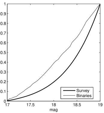
Figure 10: The magnitude cumulative distribution functions of the LMC binaries and the entire LMC survey. To show comparable populations we plot the distribution of binaries between $17$ and $19~{}I$ magnitude and of stars between $17.5$ and $19.5$.

A question that naturally arises is whether the binary frequency depends on the mass of the components. While the answer to this question is outside the scope of this study, our results allow us to examine the variation of the binary frequency in a small magnitude range. In Fig 10 we plot the magnitude cumulative distribution functions of both the binaries and of the entire survey. To display comparable populations, we plot the distribution of binaries between $17$ and $19~{}I$ magnitude and of stars between $17.5$ and $19.5$. While the stellar magnitude distribution rises exponentially, the binary distribution is almost linear. Hence, the frequency of binaries is higher for brighter stars. In fact, the frequency of binaries in the magnitude range 17 to 18 is 1.5 percent, while the frequency between 18 and 19 is 0.5% — a factor of three smaller. It is also difficult to see how the very strong variation of the rate of binaries with magnitude range could be credited to detection incompleteness only, so we suggest it is real.

4.4 The eccentricity distribution

Another feature of the whole sample that we wish to touch upon is the dependence of the binary eccentricity on the total radius. North & Zahn (2004) ignored the Algol-type eclipsing binaries of Wyrzykowski et al. (2003), and considered only eclipsing binaries that did not show considerable variation out of the eclipse. We, on the other hand, consider here all binaries with sum of radii smaller than 0.6, and therefore, naturally, have more systems with larger fractional averaged radii.

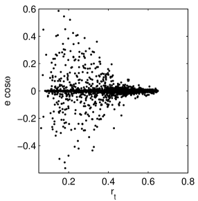
Figure 11: $e\cos\omega$ vs. the total radius

Following North & Zahn (2003), Fig 11 shows the eccentricity, multiplied by $\cos\omega$, as a function of the sum of radii. There are two minor differences between our figure and that of North & Zahn (2003). First, we present the sum of radii, while North & Zahn (2003) presented the radius, which is probably close to the average radius, as they used a value of unity for the radius ratio, and did not allow the ratio to change. Second, we use the value of $cos\omega$, while North & Zahn (2003) plotted the absolute value of this parameter. Despite these minor differences, the result obtained here is quite similar to the work of North & Zahn (2004), who found the value of the limiting averaged radius to be 0.25.

5 Discussion

5.1 The period distribution

Our analysis suggests that the binaries with B-type primaries in the LMC have flat log-period distribution between 2 and 10 days. This distribution, which was obtain after correcting for observational selection effects, is very different from the distributions of the whole samples of the SMC and the LMC eclipsing binaries (Udalski et al., 1998; Wyrzykowski et al., 2003). Evidently, correcting for the selection effects reveals a substantially different period distribution.

The period distribution derived here is probably not consistent with the period distribution of Duquennoy & Mayor (1991), who adopted a Gaussian with $\overline{\log P}=4.8$ and $\sigma=2.3$, $P$ being measured in days. Their distribution would provide within a log P interval almost twice as many systems at $\log P=1.0$ than at $\log P=0.3$ (more precisely, the factor would be 1.7), while the new derived distribution is probably flat.

It is interesting to note that Heacox (1998) reanalysed the data of Duquennoy & Mayor (1991) and claimed that $f(a)$, the distribution of the G-dwarf orbital semi-major axis, $a$, is $f(a)\propto a^{-1}da$, which implies a flat log orbital separation distribution. This is equivalent to the present probable result, although the latter refers to LMC binaries with B-type primaries, and is limited only to a very small range of orbital separation. On the other hand, Halbwachs et al. (2003, hereafter HaMUA03) analysed the spectroscopic binaries found within the G- and K-stars in the solar neighbourhood and the ones found in the Pleiades and Praesepe, and found that the log-period distribution is “clearly rising until about 10 days”.

However, HaMUA03’s sample included only a few systems with periods longer than 2 and shorter than 10 days. Actually, there were 7 such systems in the “extended sample” of nearby stars and 5 additional binaries in the Pleiades and Praesepe. In fact, if we divide these 12 binaries into two bins with equal log width we find 6 in the short-period bin and 6 in the long-period one. It is true that the correction factor of the spectroscopic binaries of these two bins is somewhat different, and therefore the distribution of this sample might still be consistent with the conclusion of HaMUA03. However, the small number of binaries with periods shorter than 10 days in the G- and K-binaries is also consistent with flat log distribution below 10 days. We verified that by building the cumulative distribution of the $\log P$ values of the 12 G- and K-binaries, and comparing it with the theoretical flat log distribution. The one-sided Kolmogorov-Smirnov test gives a probability of 0.7 that the observed distribution is consistent with the flat log distribution.

The flat log-period distribution implies a flat log orbital-separation distribution for a given total binary mass. Such a distribution indicates that there is no preferred length scale for the formation of short-period binaries (Heacox, 1998), at least in the range between 0.05 and 0.16 AU, for a total binary mass of 5 $M_{\odot}$. Alternatively, the results indicate that the specific angular momentum distribution is flat on a log scale at the $10^{19}$ $cm^{2}s^{-1}$ range.

A note of caution is in order here, as the present analysis refers to all eclipsing binaries in a given absolute magnitude range. Even if the overwhelming majority of the binaries lie on or close to the main sequence, a small unknown number of them may have gone through a mass exchange phase, which would have affected both the orbital period and the stellar radii. This is very important for the interpretation of the new result, since the most interesting quantity is probably the primordial period distribution, which was not affected by the subsequent binary evolution. In fact, Harries et al. (2003) and Hilditch et al. (2005, hereafter HiHoHa05) studied in details 50 eclipsing binaries in the SMC and found more than half of them to be in a semi-detached post-mass-transfer state. However, the binaries studied in the SMC, with limiting brightness of $B<16$, are brighter than the systems in the trimmed sample, and are composed mainly of O to B1-type primaries, while most of the primaries in the present sample are cooler B-type stars. Apparently, the fractional radii of the stars studied by HiHoHa05 is substantially larger than the typical fractional radii of the present sample. We therefore suggest that while a large fraction of the HiHoHa05 sample has gone through mass exchange, most of the binaries studied here are still on the main sequence.

We therefore suggest that the short-period B-type binaries in the LMC might have had a primordial flat log-period distribution between 2 and 10 days, and a similar feature could have been found in binaries with G-type primaries in the solar neighbourhood. Although this probable result refers to a very narrow period range, a binary formation model should account for this scale-free distribution, which might be common in short-period binaries.

5.2 The binary fraction

It would be interesting to compare the frequency of B-star binaries found here for the LMC with a similar frequency study of B stars in our Galaxy. However, such a large systematic study of eclipsing binaries is not available. Instead, a few radial-velocity and photometric searches for binaries in relatively small Galactic samples were performed. In what follows we compare the frequency derived here with results of radial-velocity searches for binaries, in samples of Galactic B stars as well as within the nearby K and G stars. In addition, we discuss the binary frequency found by the HST photometric monitoring of 47 Tuc.

5.2.1 Radial-velocity searches for binaries

Wolff (1978) studied the frequency of binaries in sharp-lined B7–B9 stars. Her Table 1 presents 73 such stars with $V\sin i<100$ km s^-1, among which 17 are members of binary systems with $P_{\mathrm{o}rb}<10$ days. This represents a percentage of $23$%, much larger than the frequency we find in the LMC. On the one hand, the frequency of Wolff (1978) may be considered a lower limit, since her sample was biased toward sharp-lined stars, because her purpose was to determine what fraction of the intrinsically slowly rotating B stars are members of close binary systems. This introduced a bias toward low $V\sin i$ values and therefore small orbital inclinations, hence lower detection probabilities, assuming the spin and orbital axes are aligned. On the other hand, the sample is magnitude limited, but the correction for the Branch bias (Branch, 1976) was not applied. The most extreme correction factor for the bias towards the more luminous binary systems, which holds for systems with two identical components, is $f=0.35$. Applying this factor to the rate of late B-type binaries with $P_{\mathrm{o}rb}<10$ days leaves a minimum frequency of $8\pm 2$%. This remains one order of magnitude larger than our frequency in the LMC.

Similar and even higher values of binary frequency were derived for B stars in Galactic clusters and associations. Morrell & Levato (1991) have determined the rate of binaries among B stars (a few O and A-type stars are also included in the sample) in the Orion OB1 association, and obtained an overall frequency of binaries with $P_{\mathrm{o}rb}<10$ days of $26\pm 6$%. There is a slight trend toward a higher rate of binaries among the early B stars than among the late ones. For B4 and earlier stars they found 60% binaries, while only $\sim 27$% of the B5 and later stars were found to be RV variables, which is reminiscent of what we find in the LMC. However, this is hardly significant as the latter frequency is based only on 3 variables.

Garcia & Mermilliod (2001) found a rate of binaries as high as $82$% among stars hotter than B1.5 in the very young open cluster NGC 6231, though in a sample of 34 stars only. Most orbits have periods shorter than 10 days. Raboud (1996) estimated a rate of binaries of at least $52$% for 36 B1-B9 stars in the same cluster, but his data did not allow him to determine the orbital periods.

These studies show that binaries hosting B-type stars tend to be more frequent in young Galactic clusters than in the field. However, even though our LMC binaries are representative of the LMC field rather than of LMC clusters, the frequency we derived appears much lower than that of the binaries in the Galactic field.

One survey of a complete, volume limited, sample of binaries in the solar neighbourhood is that of HaMUA03, who carefully studied a complete sample of K- and G-type stars, and not B stars. Out of a bias free sample of 405 in the solar neighbourhood, they found 52 binaries, 11 of them with periods shorter than 10 days. This results in a fractional frequency of $(2.7\pm 0.8)$% binaries, if one takes just the Poisson distribution to estimate the error. We therefore suggest that the fractional frequency of K- and G-type stars in the solar neighbourhood found in binaries with periods shorter than 10 days is higher by a factor of about $3.9\pm 1.9$ than the corresponding frequency of B-type stars in the LMC. The error estimate of the factor between the two fractional frequencies was derived by assuming normal distribution, and is only a coarse estimate, because of the small number statistics of the K- and G-type binaries. In fact, the difference between the two fractional frequencies is at about the $2\sigma$ level.

5.2.2 HST Photometric monitoring of 47 Tuc

A few photometric studies were devoted to the search of eclipsing binaries in Galactic globular clusters (e.g., Yan & Reid, 1996; Kaluzny et al., 1997). One of the recent photometric studies is the HST 8.3-day observations of 47 Tuc (Albrow et al., 2001), which monitored 46,422 stars in the central part of the cluster and discovered 5 eclipsing binaries with periods longer than about 4 days. Assuming a flat log-period distribution of binaries, Albrow et al. (2001) concluded that the primordial binary frequecy up to 50 years was $(13\pm 6)$%. This estimate translates into $(2\pm 1)$% for periods between 2 and 10 days. This value, derived for late-type stars, is much smaller than the frequency derived by the radial-velocity surveys of B stars, and is close to the $(0.7\pm 0.4)$% frequency we derived for the LMC.

5.2.3 Comparison between the two approaches

We conclude that the frequency of binaries we find in the LMC is substantially smaller than the frequency found by Galactic radial-velocity surveys. The detected frequency of B-type binaries is larger by a factor of 10 or more than the frequency we find, while the binary frequency of K- and G-type stars is probably larger by a factor of four. On the other hand, the binary frequency found by photometric searches in 47 Tuc is only slightly higher and still consistent with the frequency we deduced for the LMC. It seems that the frequency derived from photometric searches is consistently smaller than the one found by radial-velocity observations.

We are not aware of any observational effect that could cause such a large difference between the radial velocity and the photometric studies. The sensitivity of the two approaches depends on the ability to discover binaries with secondaries of small radii, in the photometry case, and small masses, in the case of the radial-velocity searches. In order to account for the large differences between the photometric and the spectroscopic searches we have to assume that the photometric searches detect only ten percent of the binaries and missed all the others, that could have been discovered by radial-velocity techniques. Although Wolff (1978) suggested that many short-period binaries in her radial-velocity sample have low-mass secondaries, this effect can not explain a factor of ten in the detected frequency. The discussion of the radii distribution of our sample also indicates that if such an effect is present in the LMC binaries it must be small. After all, the radial-velocity searches are not sensitive to small-mass secondaries, and they too suffer from selection effects which depends on their precision. Therefore, the large difference in the binary frequencies is probably real and remains a mystery. Obviously, it would be extremely useful and interesting to have studies of eclipsing binaries similar to the present one in our Galaxy, as well as in other nearby galaxies.

5.3 The stellar radii and the surface brightness ratios

The distributions of the two fractional radii depend strongly on the derivation of the ratio of radii, which is not well determined from the lightcurves. Still, a statistical analysis of the distributions is meaningful, given the high correlation between the true and derived $k$ values, as shown in the simulations in Paper I. The distributions of the radii show sharp peaks at the same value of 0.1, as can be seen in Fig 7, and in Fig 8 in particular. This suggests, but admittedly not prove, that our sample is mostly composed of stars with similar radii. The distribution of $J_{s}$ tends to reinforce this interpretation, since it suggests a mass ratio — hence a ratio of radii — close to one.

For the primary, the rise between $0.05$ and $0.1$ is due essentially to the limit imposed on the orbital period and to the minimum radius of a star on the ZAMS. On the other hand, the sharp rise of the secondary radius distribution up to a radius of about 0.1 is probably real. This feature of the secondary radius distribution could have been the result of a selection effect — too small a secondary results in an eclipse too shallow to be detected by the OGLE photometry. We suggest that this is not the case. The detectability limit of the sample is such that any binary with eclipse deeper than about 0.1 mag, corresponding to 10% drop in the system brightness, is included in the sample. Such a drop can be caused by a secondary with a radius which is about 0.3 of the primary radius, for inclination of $90^{\circ}$ and $J_{s}<1$. If the primary radius peaks at $\sim 0.1$, the sample is then complete for secondary radius down to about 0.03.

The peaks at about 0.1 in Fig 8 indicate that a substantial fraction of the primary and the secondary stars in the sample have radius of 2.5–3 $R_{\odot}$, assuming a typical period of 7 days in Fig 8 and a typical mass of 5 $M_{\odot}$. The sharpness of the peaks is probably caused by the magnitude limits of the trimmed sample.

5.4 The eccentricity distribution

Fig 11, with the eccentricity as a function of the sum of the two radii, displays upper and lower envelopes that can be approximated with two straight lines, with a slope of about 1.7 in absolute value. Although both the shape and slope of these envelopes may be plagued by selection biases, it is interesting to remark that the populated area corresponds to the condition

$$$$r_{t}=r_{p}+r_{s}\lesssim 0.59\,(0.85-|e\cos\omega|)\ \ .$$ (4)

This roughly generalizes the condition $r_{average}\lesssim 0.25$ to the case of eccentric systems, which cannot keep an eccentricity larger than some limiting value. This limiting value of the eccentricity depends on the stellar radii, whose sum can not be larger than a given critical fraction of the distance at periastron. Because of the $\cos\omega$ factor, it is reasonable to assume that the real relation is rather

$$r_{p}+r_{s}\lesssim 0.5\,(1-e)\ .$$

Systems with eccentricities larger than that will undergo partial tidal circularization until they satisfy this inequality; after that, tidal effects become almost inefficient. The boundary is clear-cut even though the systems do not share the same age, due to the very steep dependence of circularization time on relative radius: $t_{\rm circ}\propto(R/a)^{-21/2}$ (Zahn, 1975, 1977).

Note also that there are quite a few binaries with small radii for which the parameter $e\cos\omega$ is very close to zero. It is difficult to assume that all these system have $\cos\omega=0$. Probably those systems have circular orbits. It would be interesting to find out whether these systems were circularized during their main-sequence phase, despite their small radii, or maybe their very small eccentricity is primordial.

6 Summary

The OGLE data set has allowed us to analyze for the first time the statistical characteristics of short-period binaries with B-type primaries of an entire galaxy. We analyzed the 2580 eclipsing LMC lightcurves found by Wyrzykowski et al. (2003) and obtained orbital elements for 1931 systems. We further derived some statistical features of a trimmed sample of 938 binaries with periods shorter than 10 days, main-sequence primaries, and $I$-magnitude between 17 and 19. After correcting for the inclination effect, we find that the log-period distribution of the short-period binaries is probably flat between 2 and 10 days. Finally, we suggest that $(0.7\pm 0.4)$% of the main-sequence B-type stars in the LMC are found in binaries with periods shorter than 10 days. This is substantially smaller than the fraction found in the nearby K- and G-type stars and much smaller than that of nearby B stars. We are preparing another paper on the distribution of stars in the SMC, to find out the metallicity effect of the frequency of binaries.

This work is a further step in the study of the extragalactic binaries. Most previous studies concentrated on individual systems (see a review by Ribas (2004) and references therein). The photometry of a whole galaxy, the LMC in our case, can provide photometry of thousands of eclipsing binaries, together with distance modulus which is common to all binaries in the same galaxy. The known distances to the galaxies in the local group can provide us with absolute magnitude for a large set of early-type eclipsing binaries that is not available for Galactic binaries. Therefore, the statistical analysis of the extragalactic binaries presents great potential to our understanding of the formation of early-type binaries and stellar models.

References

- Albrow et al. (2001) Albrow M. D., Gilliland R. L., Brown T. M., Edmonds P. D., Guhathakurta P., Sarajedini A., 2001, ApJ, 559, 1060
- Alcock et al. (1997) Alcock C., Allsman R. A., Alves D., Axelrod T. S., Becker A. C., 1997, AJ, 114, 326
- Alves (2004) Alves D. R., 2004, New Astronomy Review, 48, 659
- Branch (1976) Branch D., 1976, ApJ, 210, 392
- Devor (2005) Devor J., 2005, ApJ, 628, 411
- Duquennoy & Mayor (1991) Duquennoy A., Mayor M., 1991, A&A, 248, 485
- Eggleton (1983) Eggleton P. P., 1983, ApJ, 268, 368